Mars Rover Penetrating Radar Modeling and Interpretation Considering Linear Frequency Modulation Source and Tilted Antenna

Abstract

Ground-penetrating radar (GPR) has been extensively utilized in deep-space exploration. However, GPR modeling commonly employs simplified antenna models and carrier-free impulse signals, resulting in reduced accuracy and interpretability. In this paper, we addressed these limitations by combining a tilted monopole antenna and linear frequency modulation continuous wave (LFMCW) to simulate real conditions. Additionally, a radiation-pattern-compensation back-propagation (RPC-BP) algorithm was developed to improve the illumination of the right-inclined structure. We first introduced the LFMCW used by the Mars Rover Penetrating Radar (RoPeR) onboard the Zhurong rover, where frequencies range from 15 to 95 MHz. Although the LFMCW signal improves radiation efficiency, it increases data processing complexity. Then, the radiation patterns and response of the tilted monopole antenna were analyzed, where the radiated signal amplitude varies with frequency. Finally, a series of numerical and laboratory experiments were conducted to interpret the real RoPeR data. The results indicate that hyperbolic echoes tilt in the opposite direction of the survey direction. This study demonstrates that forward modeling considering real transmit signals and complex antenna models can improve modeling accuracy and prevent misleading interpretations on deep-space exploration missions. Moreover, the migration process can improve imaging quality by considering radiation pattern compensation.

1. Introduction

Ground-penetrating radar (GPR) has been successfully utilized for subsurface structure investigations on the Earth, including cross-hole [1,2,3] and on-ground [4,5,6] GPR surveys. In addition, GPR has also been applied to deep-space planetary exploration. For instance, Lunar Penetrating Radar (LPR) onboard the Chang’e-3 [7,8] and Chang’e-4 [9,10] missions was employed to detect the subsurface geologic structure of the Moon. In the Mars exploration domain, the Radar Imager for Mars’ Subsurface Experiment (RIMFAX) implemented a linear frequency modulation continuous wave (LFMCW) GPR onboard the Perseverance Mars rover to investigate the shallow features on Mars. Notably, RIMFAX employed a single antenna for both transmission and reception via a gating technique [11]. China’s first Mars probe, Tianwen-1, was launched on 23 July 2020, and it deployed the Zhurong Mars rover at the southern Utopia Planitia of Mars on 15 May 2021. The Mars Rover Penetrating Radar (RoPeR) of the Tianwen-1 mission is equipped with a low-frequency channel (15–95 MHz) and a high-frequency channel (0.45–2.15 GHz) [12]. An LFMCW signal was transmitted by a tilted monopole antenna in the low-frequency channel [13]. In the high-frequency channel, a fully polarized Vivaldi antenna was applied [14]. Additionally, the Water Ice Subsurface Deposit Observation on Mars (WISDOM), a stepped-frequency GPR, is planned for exploring the Martian soil in 2024–2025 [15].

GPR commonly utilizes different types of excitation source signals, including carrier-free impulse, stepped-frequency, and LFMCW signals. Impulse GPR, with a long research history, was initially employed in the early 20th century to identify subsurface target characteristics [16]. Commercial GPR products based on impulse signals, such as MALA, GSSI, and SSI, have gained widespread use. Carrier-free impulse GPR employs ultra-wideband time-domain nanosecond impulses, enabling high-resolution imaging [17]. However, generating ultra-wideband instantaneous impulses poses challenges, requiring stringent radiation-frequency circuits and resulting in low radiation efficiency. Stepped-frequency and LFMCW GPR were proposed as alternatives to overcome the limitations of carrier-free impulse GPR. LFMCW GPR employs impulse compression signals with a wide bandwidth and pulse width [11,12]. Eide et al. [18] conducted simulations using a short-duration waveform and modeled the target response acquired by an LFMCW radar with a stretch processing method, without considering the antenna’s influence on the LFMCW signal. Stepped-frequency GPR utilizes a frequency jump method with a wide synthetic bandwidth and narrow instantaneous bandwidth. The stepped-frequency signal consists of coherent pulse sequences with linearly increasing frequencies, where each pulse contains a fixed frequency [15,19,20]. The choice of the transmitting signal significantly impacts GPR performance, making it a valuable research topic.

The accurate modeling of GPR data is influenced by the characteristics of antenna structures, including geometry, impedance, and materials. However, achieving realistic antenna simulation poses a challenge due to computational resources required for three-dimensional (3D) models. In GPR forward modeling, simplifications have commonly been employed, such as using isotropic point sources [1,4,21] or Hertzian dipoles [22], to streamline the calculation process. Nevertheless, these simplifications may result in decreased accuracy compared to real data [23]. To overcome this limitation, more realistic antenna models have recently been applied to improve modeling accuracy, especially in conjunction with carrier-free impulse signals [23,24,25]. In order to accurately analyze subsurface structures, GPR modeling should be capable of reproducing the spectral characteristics and target responses acquired by a more realistic GPR transmitter and receiver [18]. However, the utilization of wideband LFMCW signals and a tilted antenna configuration in the RoPeR mission has not been extensively investigated in previous studies. The impacts of antenna radiation patterns on migration images and practical solutions to compensate for these effects have not been thoroughly explored.

This study aims to enhance the understanding and interpretation of low-frequency channel RoPeR data by conducting a novel combination analysis of the LFMCW excitation source, tilted monopole antenna, and potential applications. The contributions of this work are summarized as follows:

(1)

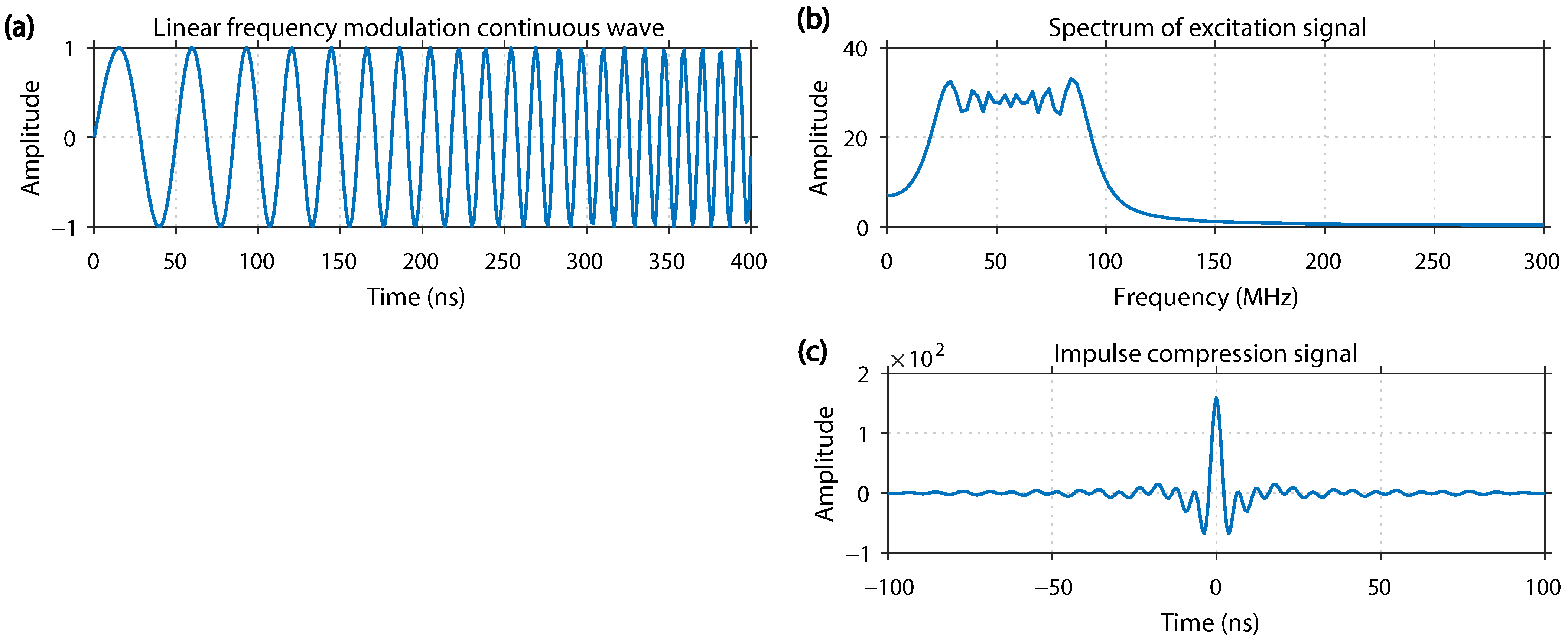
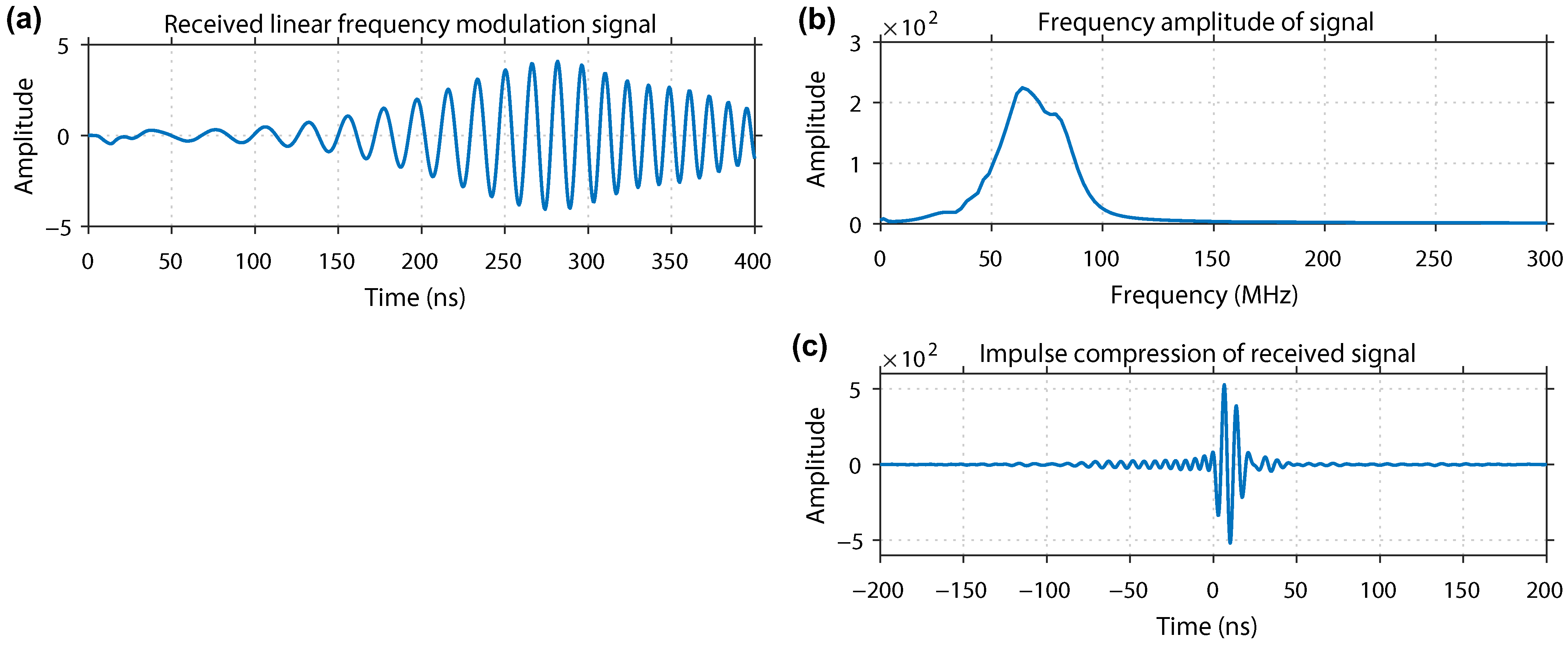
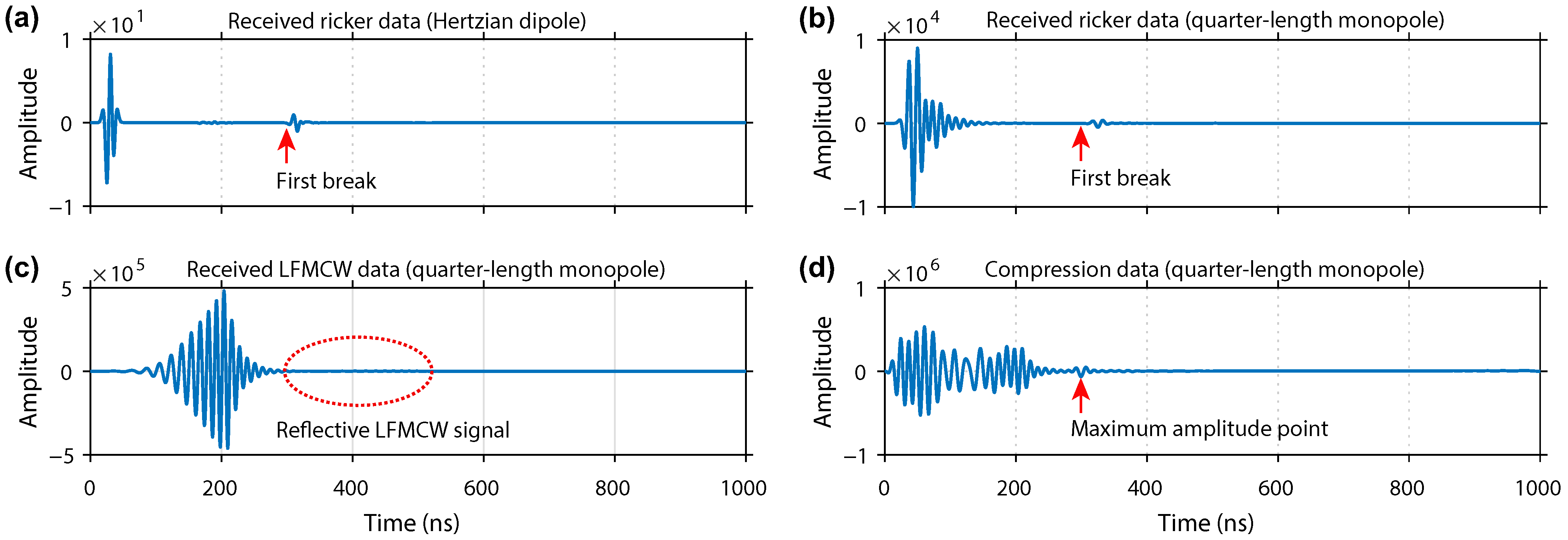
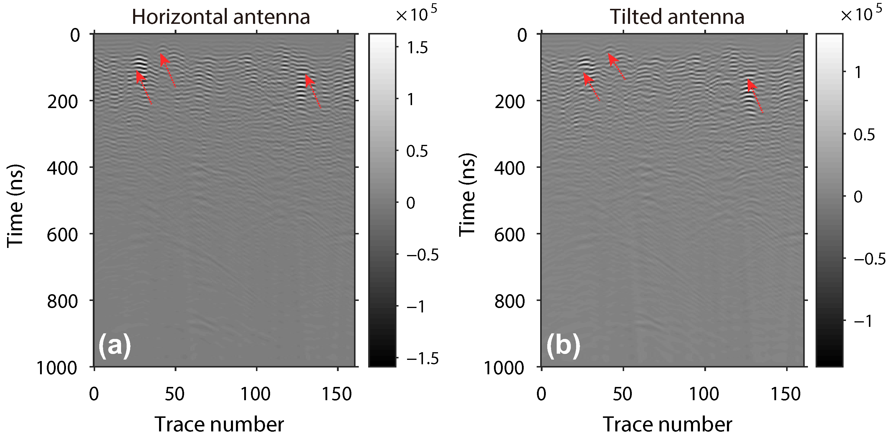
An LFMCW signal is applied to GPR forward modeling and some side lobes appear behind the main lobe after impulse compression. The assessment of the modeling approach is conducted through comparison with RoPeR data. The strong background noise appears both in synthetics and real data, which may be caused by impulse compression and antenna reflections.

(2)

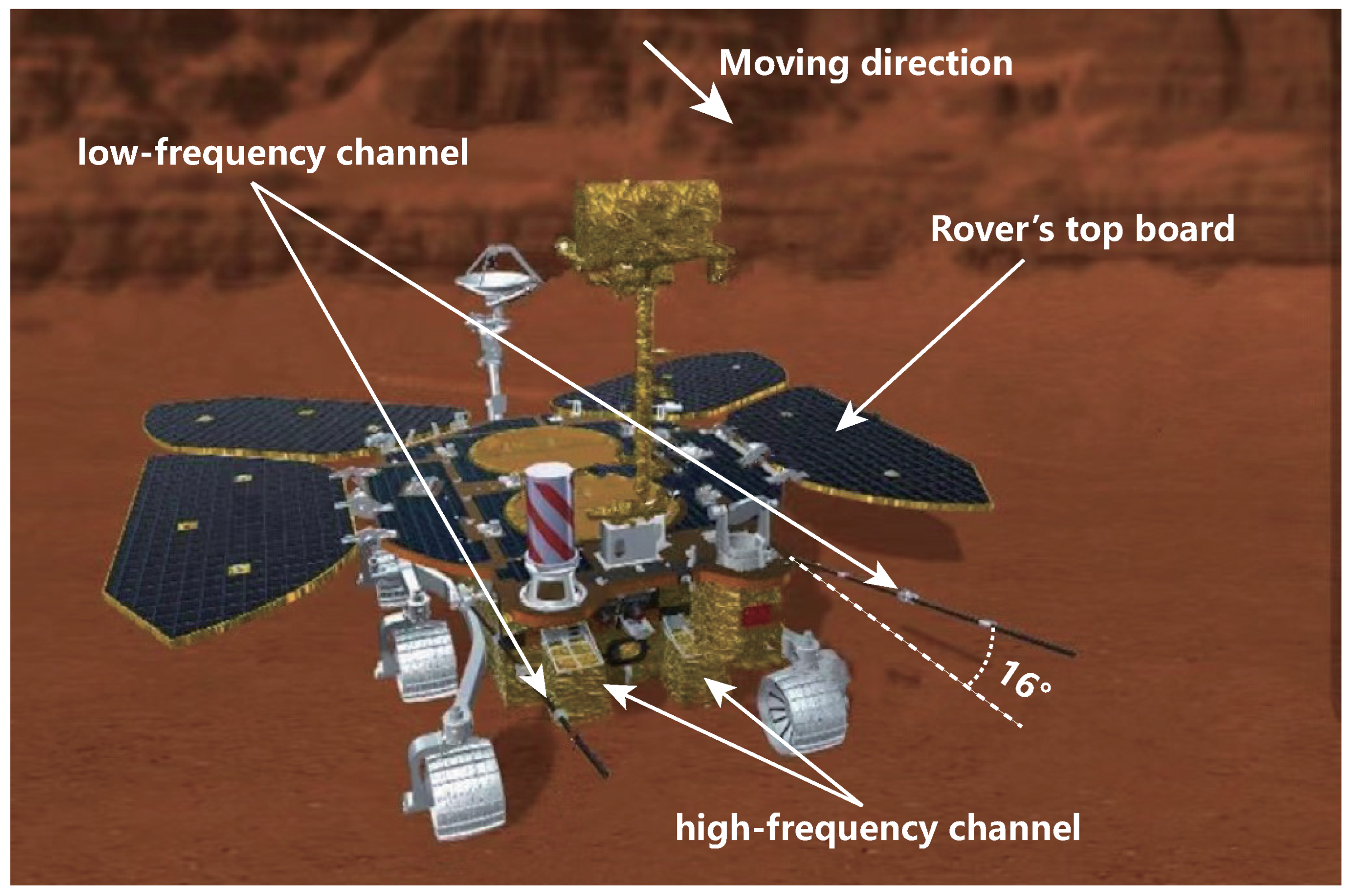
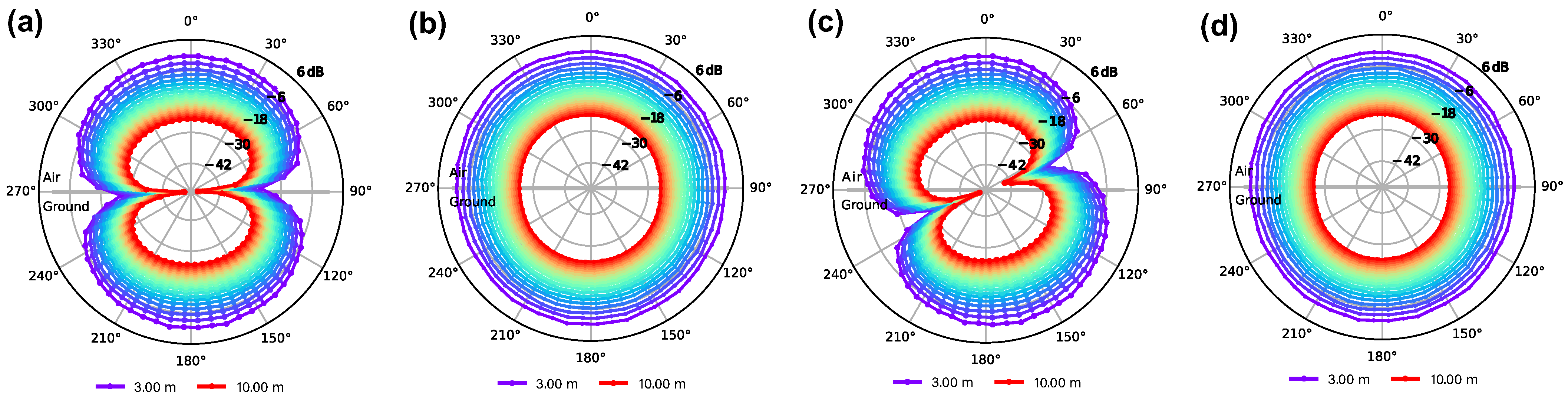
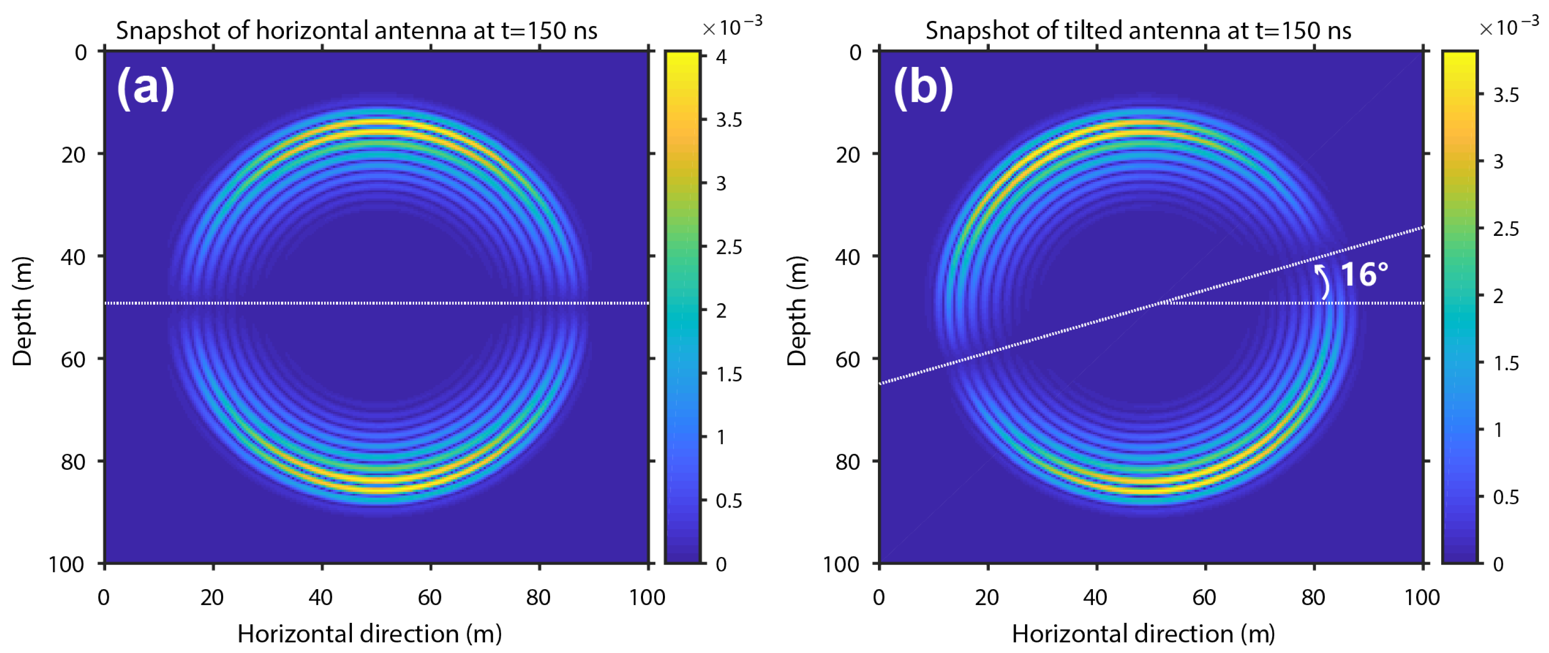
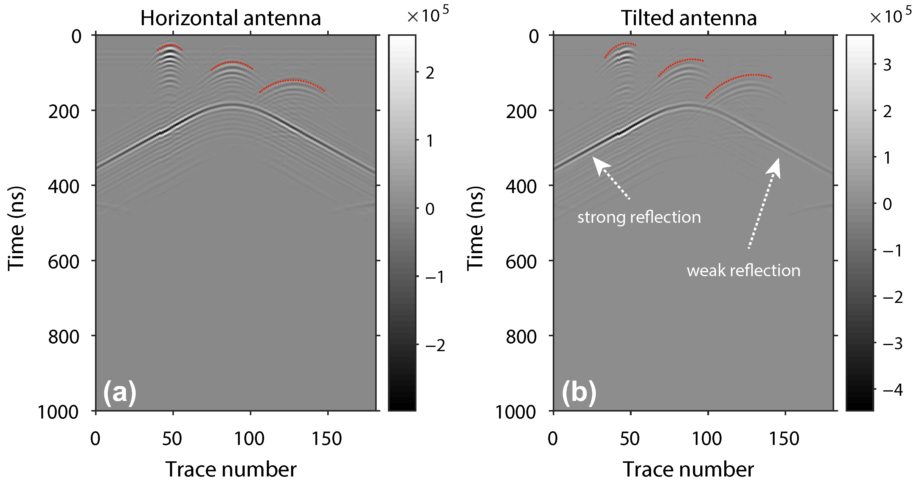
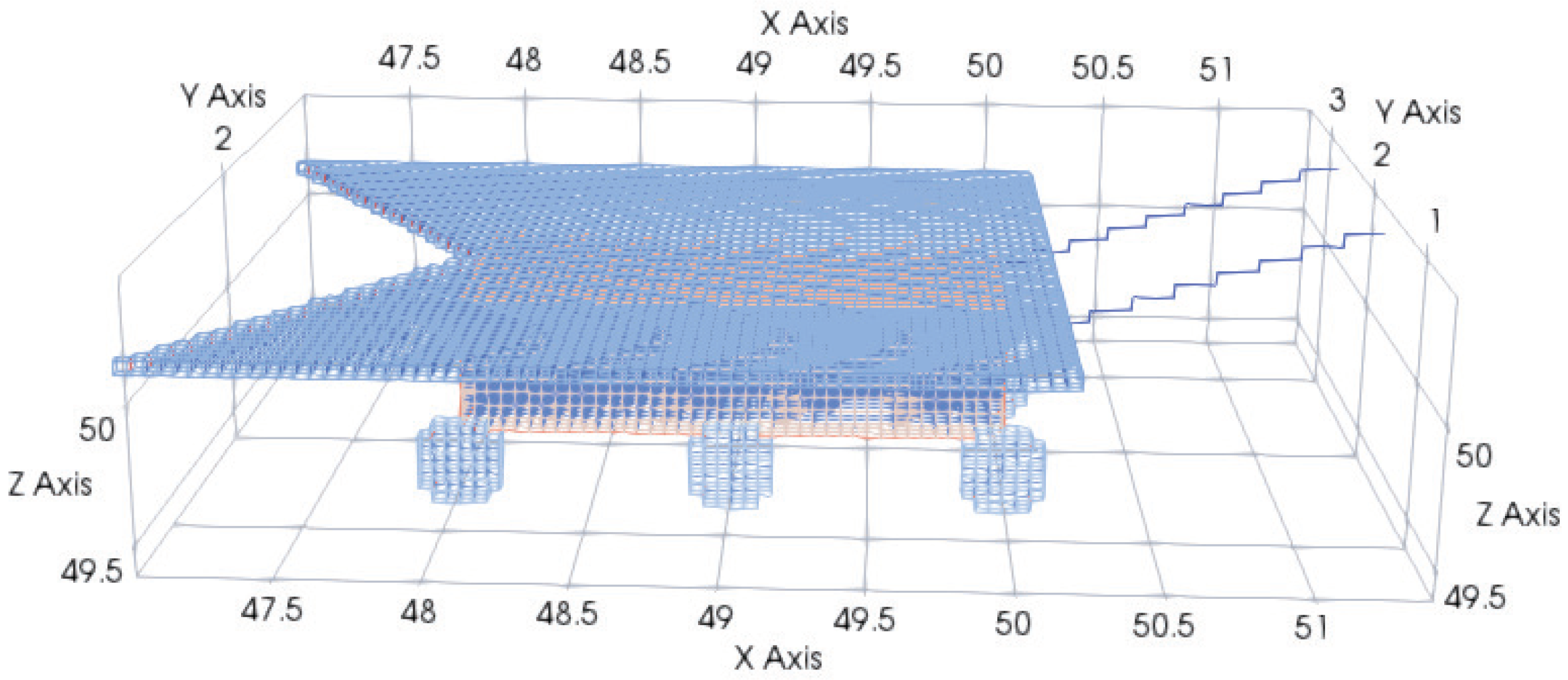
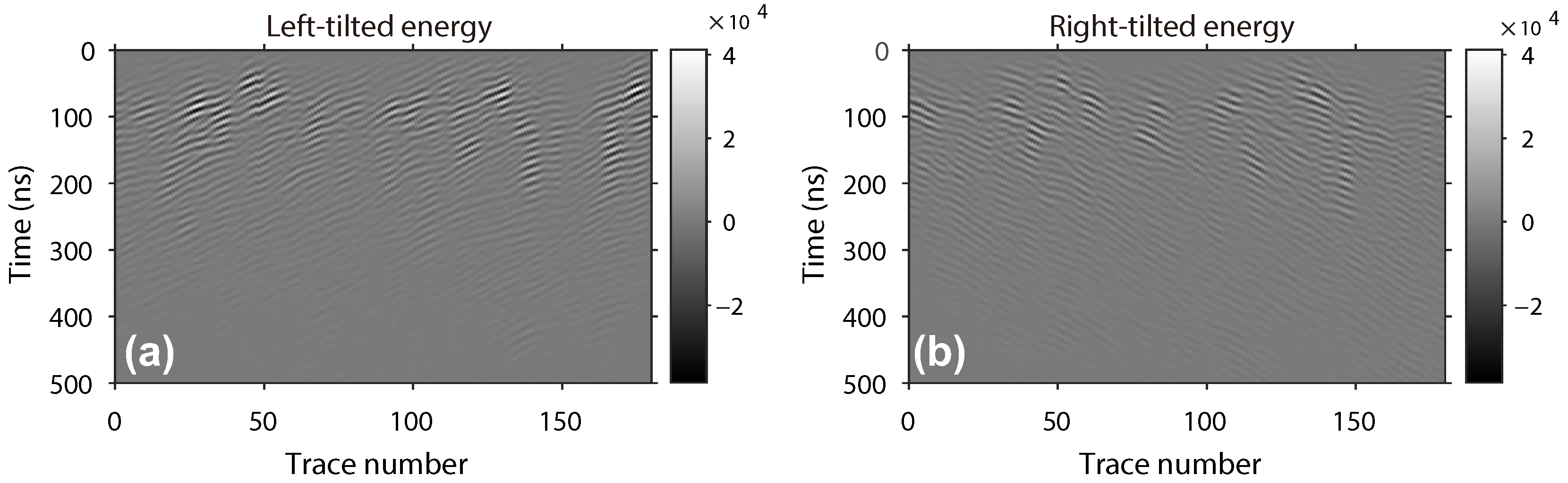
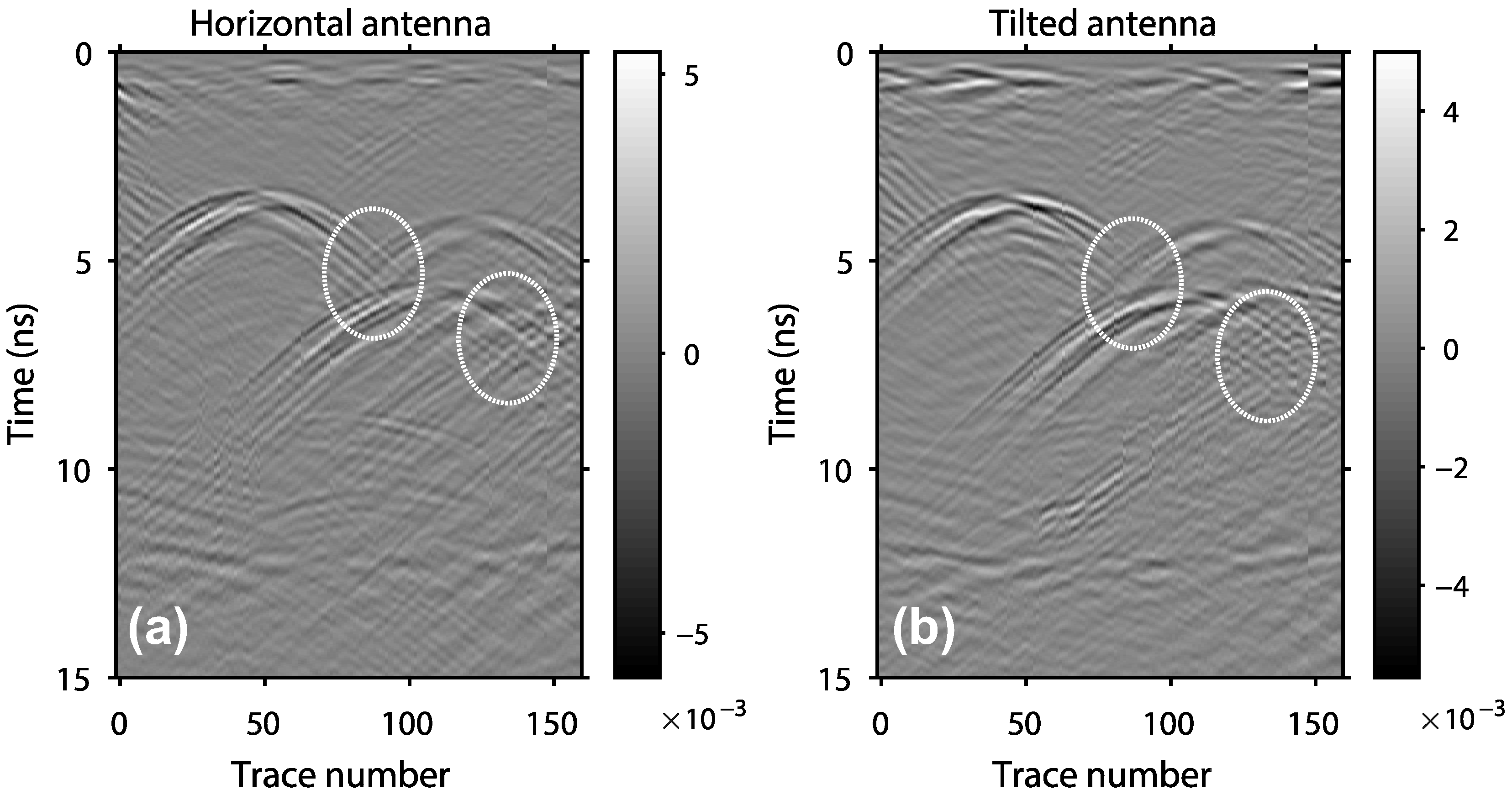
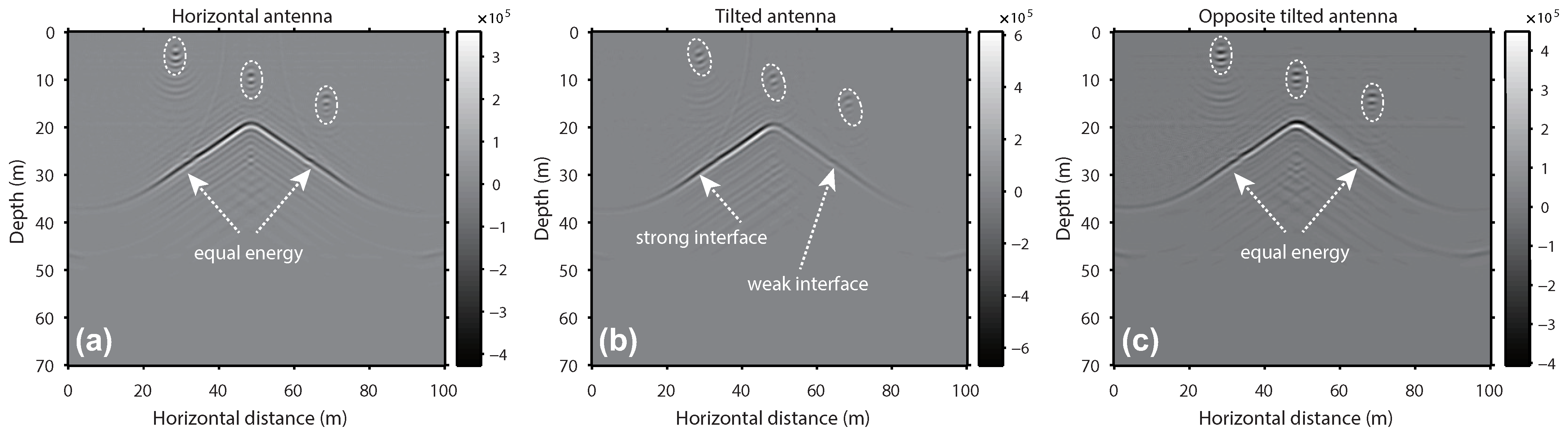
A tilted monopole antenna equipped on RoPeR is investigated by considering the antenna structure and tilted angle as well as the rover body. The modeled radargram image exhibits asymmetric hyperbolas, which is further confirmed by real observed data from the laboratory and RoPeR. The tilted antennas’ impact on back-propagation (BP) images is explored, leading to the proposal of the radiation-pattern-compensation BP (RPC-BP) method.

The remaining sections of this paper are organized as follows: Section 2 provides a brief introduction to LFMCW signals and impulse compression, followed by a discussion on the radiation pattern of tilted antenna. Section 3 presents several comparison examples involving rocky blocks. Section 4 interprets laboratory experiments and RoPeR data. Section 5 discusses the impact of a tilted radiation pattern on BP images and proposes a practical solution for radiation pattern compensation. Finally, Section 6 concludes the paper, summarizing the key findings and contributions.

2. Methodology

This section introduces the concept of LFMCW signals and focuses on the tilted monopole antenna mounted on the Zhurong Mars rover. LFMCW signals offer advantages over carrier-free impulse signals, as they provide higher average excitation energy and achieve a high-range resolution through impulse compression. Additionally, the implementation of a tilted monopole antenna displays specific RoPeR characteristics on the Martian surface. The antenna radiation pattern for LFMCW signals is thoroughly analyzed, taking into account its interpretations for the mission.

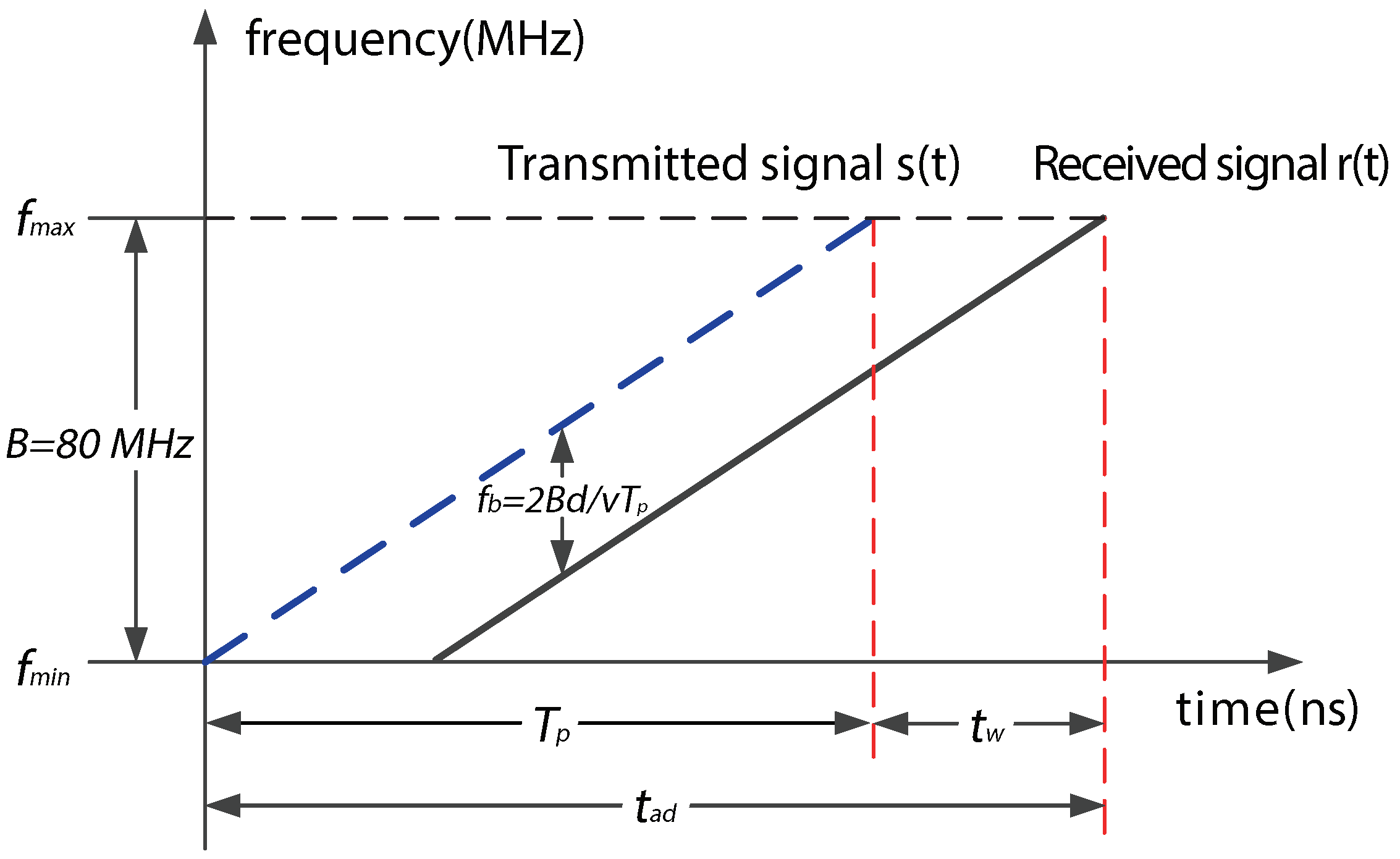
2.1. Linear Frequency Modulation Montinuous Wave

GPR systems commonly utilize narrow impulse signals in time domain, providing the advantage of an ultra-wide bandwidth. The receiving antennas in these systems often employ time-repetitive sampling techniques [16]. For instance, the carrier-free impulse LPR has been a valuable scientific payload for the Chang’e-3 [7,8] and Chang’e-4 [9,10] missions. It has been demonstrated that this type of excitation waveform is not optimal in terms of power consumption and dynamic range [26,27]. Additionally, Mars’ atmospheric conditions, with a pressure range of 0.7 to 1 kPa, are significantly denser than those on the Moon. Low-pressure discharges can easily occur in such conditions, particularly at high working voltages. To overcome these challenges, the RoPeR utilizes LFMCW and stepped-frequency signals as an excitation pulse, eliminating the need for high working voltages and improving efficiency. The rover is equipped with two antenna channels to detect different depths in Martian soil. This study specifically focuses on the low-frequency channel system with a frequency range of 15 to 95 MHz. The transmitted LFMCW signal is normalized and expressed as follows:

$$s\left(t\right)=rect(t/T_p)sin\left(2\pi (f_c+\frac{k}{2}t)t\right).$$

(1)

where $f_c$ represents the carrier frequency, B corresponds to the sweep bandwidth of the excitation signal ($B=f_{max}-f_{min}$), $T_p$ denotes the sweep duration, and k signifies the slope of the LFMCW signal in the frequency domain, which is determined by the sweep bandwidth and duration. Additionally, the rectangle window $rect(t/T_p)$ is involved:

$$rect(t/T_p)=\left\{\begin{array}{ccc}\hfill 1& & |\frac{t}{T_p}|<1,\hfill \\ \hfill 0& & elsewise.\hfill \end{array}\right.$$

(2)

The instantaneous frequency $f\left(t\right)$ of the LFMCW signal can be written as follows:

$$f\left(t\right)=f_c+kt,0<t<T_p.$$

(3)

The LFMCW signal is a non-stationary signal, with the frequency change rate denoted by $k=B/T_p$. Here, k represents how quickly the frequency of the LFMCW signal changes over time. To illustrate the excitation of the LFMCW signal, we focus on the RoPeR low-frequency channel data and provide an illustration in Figure 1. In our modeling cases, the sweep duration is $T_p=400$ ns, and the receiving antenna operates throughout the entire duration denoted by $T_{ad}=1000$ ns (the sweep duration is reduced for computational efficiency). The penetrating time window is set as $T_w=600$ ns. The bandwidth is defined as $B=f_{max}-f_{min}=80$ MHz. An echo is received from a distance d in a homogeneous model with a velocity of v. Taking the two-way travel into account, the delayed time is given by $t=2d/v$. The received delayed signal has a lower frequency than the currently transmitted signal. By multiplying the received signal with the currently transmitted signal, a baseband signal is obtained with a frequency equal to the difference between the two signals. This frequency difference, known as the beat signal in Figure 1, is proportional to the delay time and, thus, the distance range to the reflector. The proportionality constant is determined by the ratio of the sweep bandwidth to the sweep duration. The frequency of beat signal can be expressed as $f_b=2Bd/\left(v{T}_p\right)$, corresponding to the distance from the source to target by pulse compression with stretch processing [11].

Figure 2 depicts the LFMCW signal used in the low-frequency channel. In Figure 2a, the time-domain representation of the LFMCW signal is presented, with a duration of $T_p=400$ ns. The signal exhibits a frequency increase from 15 to 95 MHz over time. This long-duration excitation of the LFMCW signal allows for increased energy compared to carrier-free Ricker or Gaussian wavelets. The spectrum of the LFMCW signal is illustrated in Figure 2b using Fourier transform. The center frequency of the LFMCW signal is observed to be 55 MHz.

Compared to carrier-free impulse GPR, the data processing of LFMCW system GPR is more complex. In addition to stretch processing, a matching filter is another way to obtain the high-resolution compression impulse. The time-domain match filter $h\left(t\right)=s(-t)$ is expressed as follows:

$$r\left(t\right)=r_l\left(t\right)\ast h\left(t\right)={\int }_{-\infty }^{\infty }{r}_l\left(\tau \right)s(\tau -t)d\tau$$

(4)

The compressed impulse $r\left(t\right)$ is obtained through the convolution of the received LFMCW signal $r_l\left(t\right)$ with the system impulse response $h\left(t\right)$. Figure 2c illustrates the compressed impulse in a special case where $r\left(t\right)=s\left(t\right)$, indicating that match filtering is equivalent to autocorrelation. In this scenario, the delayed time t and distance d are both set to 0. It can be observed that the impulse compression algorithm introduces side lobes around the main lobe at $t=0$. In general, there is a trade-off between the bandwidth and pulse width in the cases of Ricker or Gaussian wavelets. As the frequency increases, the pulse width decreases. However, the bandwidth and pulse width of the LFMCW signal are decoupled. As depicted in Figure 2a,c, the compressed impulse exhibits a higher resolution and amplitude. The LFMCW signal in time domain provides increased energy, resulting in a higher signal-to-noise ratio (SNR).

2.2. Tilted Monopole Antenna

The antenna plays a crucial role in the RoPeR system and explains how electromagnetic signals are transmitted to the underground. However, most modeling and applications are designed based on isotropic point or Hertzian dipole sources, which do not match real situations. The antenna structure significantly influences electromagnetic radiating performance. Compared with the real observed data, an oversimplification of the antenna model may lead to inaccurate synthetic data modeling. In the case of the RoPeR low-frequency antenna, it is mounted on the bottom surface of the rover’s top board [12]. The antenna has a length of 1.35 m and a diameter of 0.12 m. The central frequency of the transmitted LFMCW signal is set at 55 MHz. We consider the vacuum velocity as $v=3\times {10}^8$ m/s, resulting in a quarter-wavelength of $l=v/4f=1.36$ m. It should be noted that the antenna is not oriented horizontally but rather at an angle of $16°$ from the horizontal direction. This is indicated by the dashed white line in Figure 3 [28].

Two simplified models of the horizontal and tilted monopole antennas were constructed to analyze radiation patterns, as shown in Figure 4. The ground plane size is $0.2\times 0.2$ m in the y and z directions. Numerical simulations and comparisons were performed, revealing that the ground plane size affects antenna radiation patterns gain. However, it does not impact the characteristics of elevation plane patterns. To enhance the antenna’s bandwidth, a material with a conductivity of $\sigma =10$ S/m was utilized to reduce antenna current reflections. The load and feed points were positioned at the endpoint closest to the RoPeR.

Radiation pattern images were generated at a frequency of 55 MHz to illustrate the radiation performance of both horizontal and tilted monopole antennas in Figure 5. Different color lines represent distances ranging from 3 to 10 m. The closer positions show higher radiation energy indicated by blue lines. In the case of the horizontal monopole antenna shown in Figure 5a, the maximum radiation direction is 180°, indicating that electromagnetic waves propagate orthogonally into the underground. However, due to the antenna’s tilted orientation, the elevation plane pattern also demonstrates tilted characteristics in Figure 5c. Specifically, it shows strong and weak radiation directions at 164° and 74°, respectively. The strongest radiation direction is not directly beneath the antenna. Instead, the electromagnetic wave is incident on the ground obliquely and in an upward direction. The azimuth plane radiation patterns of horizontal and tilted antennas show similar characteristics in Figure 5b,d.

We conducted tests using two types of antennas: a horizontal monopole antenna and tilted monopole antenna, in a homogeneous model. The excitation signal utilized is a Ricker wavelet impulse with a center frequency of 55 MHz. The antennas are located at the center of coordinates $source=(50,10,50)$ m. We obtained two-dimensional (2D) snapshot slices along the $y=10$ plane. At the time $t=150$ ns, the snapshots of horizontal and tilted monopole antennas are depicted in Figure 6. In Figure 6a, the radiation energy of the horizontal monopole antenna appears weak in the horizontal direction. However, the radiation energy is observed to rotate counterclockwise by $16°$ compared to the horizontal antenna in Figure 6b.

The radiation performance of antennas varies depending on frequency. A quarter-wavelength antenna operates on a frequency range of 15 to 95 MHz, with a bandwidth of $B=80$ MHz. Figure 7a shows the voltage standing wave ratio (VSWR) characteristics of the antenna. The lowest VSWR is 1.68 at the frequency $f\approx 55$ MHz. The reflective parameter is $\tau =0.2537$ and $93.56\%$ electromagnetic energy is radiated. The VSWR is over 10 for the low-frequency channel operating at 15 MHz, and only a small portion of the energy is radiated from the antenna. Figure 7b provides the S11 parameter, which also indicates that the monopole antenna works best at the frequency $f\approx 55$ Mhz. The radiation property analysis shows that a quarter-wavelength monopole antenna may lead to significant reflection for the low-frequency components.

In addition, we applied a homogeneous model to demonstrate the antenna response to the LFMCW signal. The transmitting and receiving antennas are positioned 1 m apart at the center of the model. The monopole transmitting antenna radiates electromagnetic energy into the vacuum. The central frequency of the source signal is $f_c=55$ MHz, as shown in Figure 2a. The received signal in Figure 8a is detected by a parallel antenna. The amplitude of the received signal varies for different frequencies, with the low-frequency components exhibiting weaker energy compared to the high-frequency components. The spectrum of the received signal is depicted in Figure 8b, where the low-frequency (15 MHz) and high-frequency (95 MHz) components are filtered and displayed. Generally, low-frequency waves experience more attenuation than high-frequency waves. The compression impulse in Figure 8c shows a time shift caused by the one-meter distance between the transmitting and receiving antennas. The trailing portion following the primary impulse is caused by reflective currents in a quarter-wavelength antenna.

3. Forward Modeling

To show the responses of different antennas and excitation signals, a three-dimensional (3D) toy model is constructed in Figure 9. The model size is 100 × 20 × 70 m along the x, y, and z coordinates and is discrete with a grid spacing of $\Delta x=\Delta y=\Delta z=0.1$ m, resulting in a total of 140,000,000 elements. Perfectly matched layers (PMLs) absorb boundary reflections. The relative permittivity and conductivity of the atmosphere are ${ϵ}_r=1$ and $\sigma =0$, respectively. The top layer permittivity and conductivity are ${ϵ}_r=1.73$ and $\sigma =3.73\times {10}^{-5}$ S/m, respectively. Three spherical targets with a radius of 1 m are included, characterized by a relative permittivity of ${ϵ}_r=7.00$ and a conductivity of $\sigma =6.08\times {10}^{-4}$ S/m. These targets are located at ${\mathbf{x}}_{\mathbf{1}}=(30,10,3)$, ${\mathbf{x}}_{\mathbf{2}}=(50,10,8)$, and ${\mathbf{x}}_{\mathbf{3}}=(70,10,13)$, with increasing depths. Furthermore, two tilted interfaces are constructed at the model bottom, with electrical parameters of ${ϵ}_r=9.00$ and $\sigma =2.61\times {10}^{-4}$ S/m. The recent research has indicated that the loss tangent value of Martian regolith at the Tianwen-1 landing site is $0.{0174}_{-0.0053}^{+0.0053}$ [29]. The loss tangent value of 0.0174 is used to evaluate the conductivity of $\sigma =5.246\times {10}^{-5}$. Therefore, the conductivity ranges from ${10}^{-5}$ to ${10}^{-4}$ S/m in our cases. All comparisons presented in this subsection are based on the rocky block model depicted in Figure 9.

In this study, complex transmitting and receiving antennas require 3D modeling, which requires more computational resources. We utilized open-source electromagnetic simulation software named gprMax [30]. MPI and CUDA were combined to improve modeling efficiency [31]. Forward modeling was performed on a distributed cluster. The computational node contains 256 GB of memory and two Intel(R) Xeon(R) Gold 6240 CPUs each running at 2.60 GHz and with eighteen cores. There are two RTX 3090 GPUs with each card having 24 GB of memory. The computational node and every GPU consume 10.7 GB of memory for the current toy 3D model. Each A-scan modeling takes about 3 min, and a total of 270 min is required for a radargram with 181 traces by two GPU solvers. Mesh generation takes a lot of processing time on CPU, and forward calculation by GPU is efficient.

3.1. Modeling Based on Ricker Wavelet and LFMCW Source

In this subsection, we conducted a comparison between a Ricker wavelet (transmitted by Hertzian dipole and quarter-wavelength monopole antennas) and LFMCW (excited by a quarter-wavelength monopole antenna). The excitation is provided by an x-polarized voltage source with an internal resistance of 36.5 Ohms. The Ricker wavelet has a maximum amplitude of 1 volt and a center frequency of 55 MHz, while the LFMCW signal has an amplitude of 1 volt as well. To highlight reflected echoes, the received signals are subjected to a linearly increasing gain. The time sampling interval is ${\Delta }_t=0.2407$ ns, and total recorded time length is 1000 ns. A radargram is formed by systematically moving the transmitting and receiving antennas in equal intervals of 0.5 m from 5 to 95 m, allowing us to visualize the differences between the Ricker wavelet and LFMCW excitation sources.

Figure 10 displays the radargram after amplitude compensation, providing deeper information. In Figure 10a, the recorded radargram of the Ricker source excited by the Hertzian dipole antenna reveals clear airwave and surface-related reflections without significant tailing. Three reflected hyperbolas caused by rocky blocks at different depths are marked with red circles. Additionally, echoes from the tilted interface are prominent. Figure 10b shows the radargram of a Ricker wavelet transmitted by a quarter-wavelength monopole antenna. Horizontal banding noise is visible only in the early stages, attributed to antenna current reflection. Reflections from the rocky blocks are scarcely observed during the initial stage. In Figure 10c, the radargram transmitted by the LFMCW source demonstrates continuous excitation over an extended period. Echoes from rocky blocks and tilted interfaces can be faintly observed. Figure 10d presents the impulse compression result of Figure 10c. The signal displays significant horizontal banding in the form of side lobes after impulse compression, with energy decreasing over time. The hyperbolas from the spheres are concealed by the strong-energy side lobes, and only a portion of the interface reflection is apparent. Therefore, both the current reflection in the antenna and the side lobes of impulse compression may contribute to horizontal banding in radargrams. The white wiggle lines in radargrams indicate the positions where A-scans are displayed in Figure 11.

The transmitting and receiving antennas are located at ${\mathbf{x}}_{\mathbf{s}}=(80,9.5,-0.8)$ and ${\mathbf{x}}_{\mathbf{r}}=(80,10.5,-0.8)$ in Figure 9. Figure 11a is the A-scan plot of the Ricker wavelet excited by a Hertzian dipole. There is no tailing signal in the recorded data. Figure 11b exhibits a short tailing due to antenna reflective current and ground reflections. Figure 11c is the A-scan of LFMCW signal and Figure 11d is impulse compression echo. Comparing Figure 11a,d, we found the first arrival of the Ricker wavelet is delayed, which is caused by different counting methods. Two-way travel time in Figure 11b takes into account the first break. However, the impulse compression in Figure 11d is measured in time at the maximum amplitude. Additionally, the side lobe of impulse compression continues for a longer period following the primary reflective wave. LFMCW radiation offers superior efficiency. Therefore, the amplitudes of Ricker and LFMCW sources show significant differences in Figure 11a,d, in which the amplitude of impulse compression echoes is much higher than that of the Ricker source.

3.2. Modeling Based on Horizontal and Tilted Antennas

A horizontally or vertically placed Hertzian dipole is typically implemented in GPR forward modeling. Although the low-frequency antenna mounted on the rover is tilted (like the Chang’e-3 and Chang’e-4 missions [10,32]), previous research has not explored how the antenna structure and radiation patterns influence measured radargrams. In fact, GPR antennas may significantly affect electromagnetic wave propagation in underground space. Monopole antennas radiate more energy in the perpendicular direction of the moving path. They do not have a concentrated radiation pattern, as shown in Figure 5.

The response descriptions of rocky blocks and inclined interfaces to horizontally placed and tilted monopole antennas are shown in Figure 12. First, the horizontally placed antenna can record the strongest echoes when the antenna is directly above block targets in Figure 12a. The reflective signals would decrease with an increasing distance between targets and RoPeR. The left and right sides of hyperbolic echoes are the same in strength for horizontal antennas. However, the situation is different for the tilted antenna in Figure 12b. The strongest echoes are measured by a tilted antenna when RoPeR is located at the upper left of the target, leading to unsymmetrical hyperbolic reflectors. The area covered by RoPeR can be described by its beam width. The hyperbolic amplitude of the left side is higher than that of the right side. The phenomenon may not be caused by subsurface geologic structures but by antennas. In Figure 12c, the horizontal antenna exhibits the same response on left- and right-inclined interfaces. The tiled antenna shows strong echo energy on the left-inclined interface rather than the right one in Figure 12d.

As discussed in the last subsection, the strong horizontal background banding is caused by direct airwaves, the current reflection in antennas, and the side lobe of impulse compression. This background banding noise did not contain any underground information. Therefore, we subtracted background noise from radargrams to show reflected echoes [8,9]. The background-removal radargrams of horizontal and tilted monopole antennas are shown in Figure 13. Classical hyperbolic reflections are marked in Figure 13a,b by red dashed curve circles. Shallow targets have less influence on large-offset data. In Figure 13a, the blocks’ reflective hyperbolas is left and right symmetric. The strongest reflection is directly above buried targets. There are also strong surface-related multiples between the ground surface and shallow rocky blocks. The left- and right-inclined interfaces exhibit similar reflections. However, the reflective hyperbolas are tilted to the left, and the right-side energy is weak in Figure 13b, which corresponds to the theoretical analysis in Figure 12b. In addition, inclined interfaces measured by the tilted antenna exhibit stronger reflection in the left-inclined structure.

RoPeR moves from the left to right in Figure 12, where the two-way travel time for a surface position is given by $t=2\sqrt{x^2+h^2}/v$, with x representing the horizontal offset between the antenna and rocky targets, h representing the depth of buried targets, and v representing electromagnetic wave propagation speed in the subsurface medium. The travel time depends on the horizontal offset and depth. The zero-offset two-way travel time is $t_0=2h/v$ when RoPeR is directly above rocky targets. The time–distance curve can be described by the standard hyperbolic equation as shown in Equation (5).

$$\frac{t^2}{4h^2/v^2}-\frac{x^2}{h^2}=1$$

(5)

The radargram reveals distinct hyperbolic characteristics for targets at different depths. The kinematic properties, represented by travel time, are described by Equation (5), which is a hyperbolic equation focused on the time axis. The time–distance curve exhibits the same asymptote of $t=\pm 2/v$ for targets at different depths. But it is not the same for vertices of $t_0=2h/v$ and top curvature radius of $\rho =hv/2$. As a result, hyperbolas associated with deeper targets appear wider. By considering the dynamic features (amplitude and phase) in Figure 13, shallower targets only have imprints on the small-offset data, while deeper targets can influence data on larger offsets.

3.3. Mars Rover Influence on Recorded Data

Angelopoulos et al. have explored the artifacts caused by signal interaction with a rover body [33], in which a metal plate is employed to simulate the LPR body. A variable height was explored to show horizontal banding noise formation. In addition, a varied distance between the plate and antenna was tested. The rover shows obvious imprints on recorded data. Energy reflected either directly from the rover or after reflection from the surface is expected to be the most significant source of data artifacts. Horizontal banding and multiple reflections (i.e., repeated reflections from one target at successively increased depths) between the rover and subsurface targets are of particular concern. It is possible to misinterpret these types of noise as stratigraphy or numerous buried objects [34]. Following the structure of the Zhurong rover, we build a Mars rover model in Figure 14 by uniform grids. The rover mainly consists of four parts, including the top board, body, six wheels, and two antennas. The size of top board is $3\times 3\times 0.05$ m in the x, y, and z directions. The vertical distance between the top board and the ground is 0.8 m. The permittivity and conductivity of top board are ${ϵ}_r=7$ and $3\times {10}^{-4}$ S/m, respectively. The rover body size is $2\times 1\times 0.5$ m in the x, y, and z directions. The rover body’s permittivity and conductivity are 3 and $2\times {10}^{-2}$ S/m. The radius of the wheels is 0.15 m and the space between adjacent wheels is 1 m. The length of the modeled tilted antennas is 1.35 m and the inclined angle is about $16°$ between the antenna and the horizontal level. Both the rover wheel and monopole antenna are constructed in metal.

Considering the influence of the Mars rover’s top board and body, the low-frequency radargrams before and after horizontal banding removal are shown in Figure 15. The radargrams with the Mars rover’s top board contain some tailing behind the primary reflection in Figure 13b and Figure 15b. The rocky block’s response contains the side lobe interfaced with the rover body, which is marked by multiple red dashed lines. In addition, the response signal of rocky blocks tilts to the left in Figure 15 caused by the tilted antenna. In contrast with previous research results [33], the rover’s side plate imprints are not significant. This is because the RoPeR equipped on the Zhurong rover utilized HH polarization surveys to minimize artifacts.

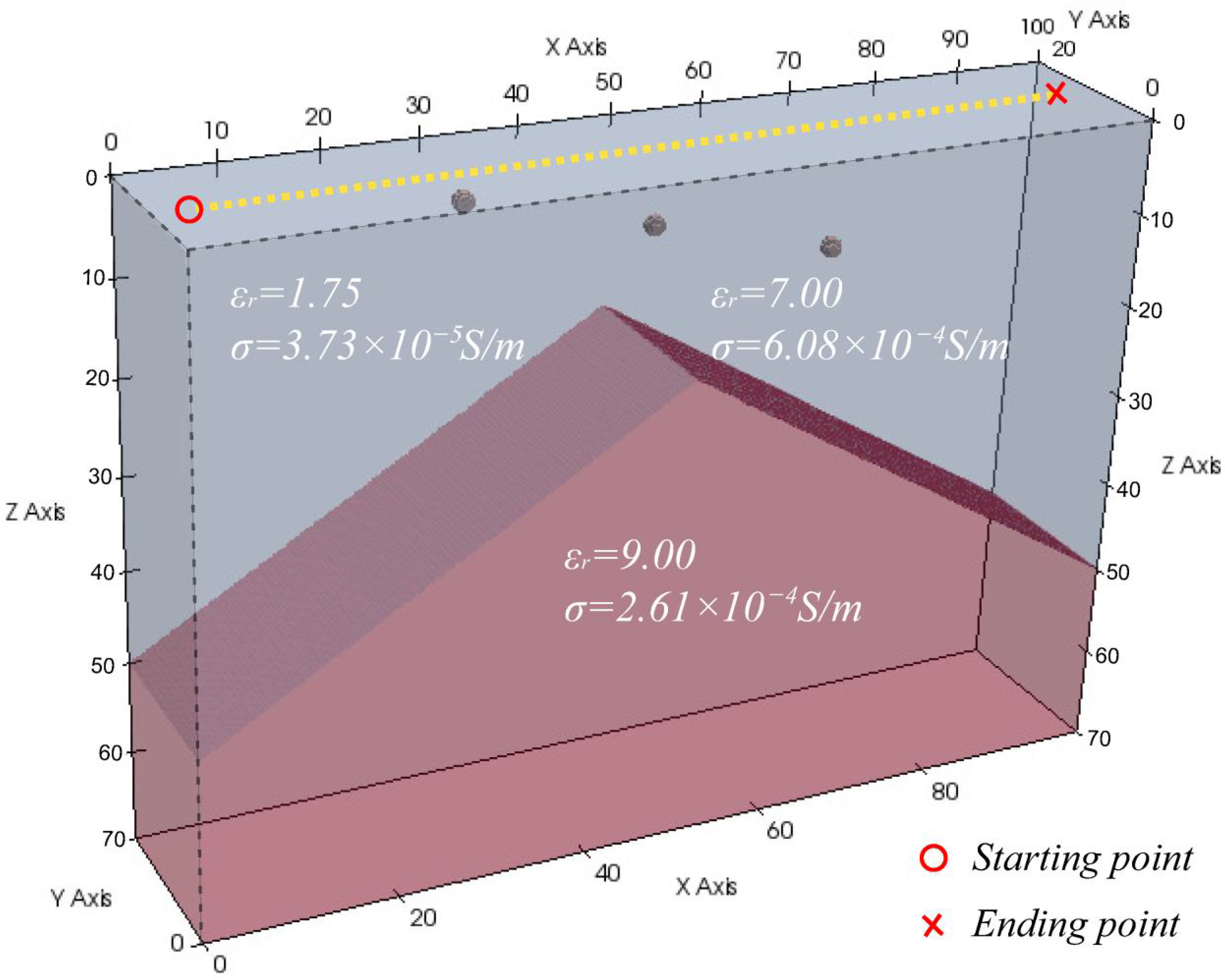
3.4. Complex Subsurface Structure Modeling

Referring to the Martian subsurface model of the Zhurong rover landing site given by Li et al. [13], we built a 3D model containing different sizes of rocky blocks, as shown in Figure 16. The model size is 100 × 20 × 80 m along the x, y, and z axes. The model is discrete with $1000\times 200\times 800=160,000,000$ elements in total and the memory cost is 11.4 GB for forward simulation. Figure 16 only shows the subsurface part with a depth of 70 m; the atmosphere layer with a thickness of 10 m and deeper structure of more than 70 m are not shown in this model. The background permittivity is gradually increased from 2.28 to 8.69 and the background conductivity varies from $0.43\times {10}^{-4}$ to $1.61\times {10}^{-4}$ S/m. The subsurface structure is divided into three layers. The first layer’ thickness is 8 m, with an average dielectric permittivity ranging from 3 to 4. This layer contains some moderate blocks with sizes ranging from 0.25 to 1.00 m. The second layer is a fining-upward sequence within depths from 8 to 30 m, which includes some small rocks from 8 to 20 m and some relatively large blocks from 20 to 30 m. The small target sizes range from 0.25 to 0.7 m and bigger targets vary from 0.25 to 2 m in radius. The bottom layer, extending from 30 to 70 m, is also a fining-upward sequence layer, in which small-sized rocks are from 0.25 to 0.75 m and big-sized rocks are from 0.25 to 2.25 m in radius. The detailed information can be found in

Table 1. Three-dimensional complex model parameters in depth, quantity, radius, relative permittivity, and conductivity.

Layers	Depth (m)	Quantity	Radius (m)	Permittivity	Conductivity (S/m)
1st layer	0∼8	80	0.25∼1.00	1.75∼10	(0.37∼3.35) $\times {10}^{-4}$
2nd layer	8∼30	400	0.25∼2.00	1.75∼13	(0.37∼3.73) $\times {10}^{-4}$
3rd layer	30∼70	260	0.25∼2.25	1.75∼13	(0.37∼3.73) $\times {10}^{-4}$

. There is no obvious interface between different layers [13]. The yellow dashed line in Figure 16 shows RoPeR’s moving path. The red rover and cross represent the starting and ending positions of the survey line. A stochastic rough surface is built with a depth of 1.8 m and a peak of 0.2 m (the base height is 0 m) to simulate Mars’ complex ground surface.

The modeling radargrams of horizontal and tilted antennas with rover impact are shown in Figure 17. The spatial sampling interval is about ${\Delta }_r=0.5$ m and the trance number is 181 in total from 5 m to 95 m. The LFMCW is transmitted by the horizontal and tilted monopole antennas in this case so as to simulate a real data processing flow. A matched filter is used to improve the SNR of echoes from subsurface reflectors. The radargrams after impulse compression are exhibited. The direct airwaves and reflected waves from the surface are strong and almost cover the all echoes from subsurface targets. Additionally, impulse compression introduces low-energy side lobes that follow directed air events. Those side lobes would also significantly influence reflected echoes reorganizations. The horizontal banding (direct airwaves and reflected echoes from the surface) are subtracted in Figure 17 [8,9,13]. In Figure 17, the hyperbola recorded by the horizontal antenna is left–right symmetric. In Figure 17b, the left-side energy of the hyperbola is stronger than that of the right side, which was caused by the tilted monopole antenna.

In complex subsurface models of Mars, it can be challenging to evaluate the directional characteristics of echoes from radargrams, particularly when hyperbolas intersect each other. Radargrams can be separated using a 2D directional filter to quantitatively assess the coherency of scattering or reflection waves along the same phase axis. The filter operator $h_l$ is defined as $h_l=[0,1,0;1,0,-1;0,-1,0]$ for left-inclined structures, where the maximum amplitude energy is obtained at the $45°$ interface. Similarly, the filter operator $h_r$ for right-inclined structures is represented as $h_r=[0,1,0;-1,0,1;0,-1,0]$, with the maximum amplitude energy obtained at the $135°$ interface. These two filter operators are orthogonal in two directions. Taking the radargram in Figure 17b as an example, we applied directional filters to separate echoes. The separated left-inclined radar echoes are shown in Figure 18a, while the separated right-inclined radar echoes are displayed in Figure 18b. It can be observed that the left-inclined radar echoes have a slightly stronger energy compared to the right-inclined radar echoes. The power ratio between the two types of echoes, denoted as $R=r_l^2/r_r^2$, is calculated to be 1.21 in this case.

4. Analysis of Laboratory and Mars Rover Data

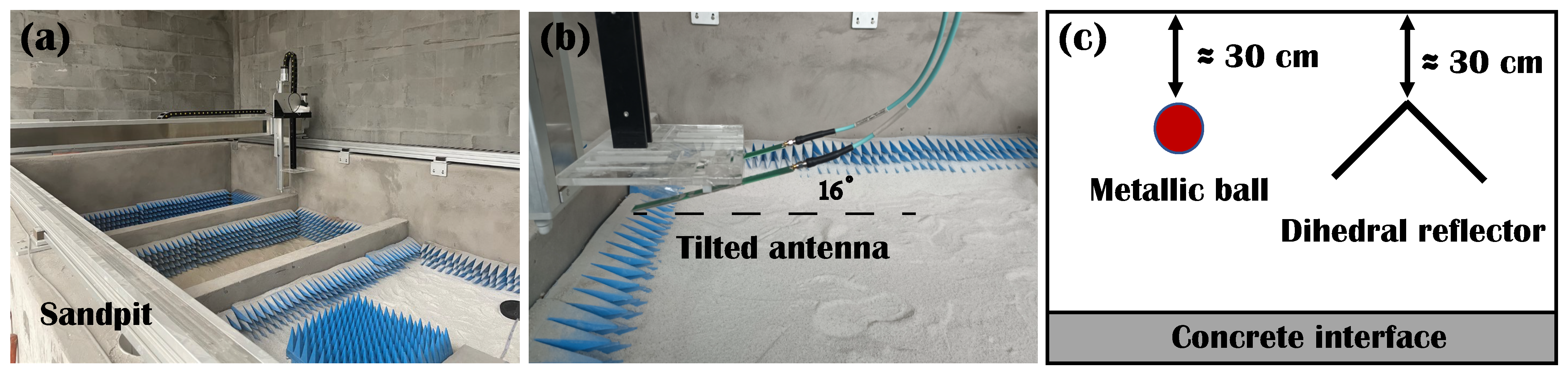
4.1. Laboratory Data Analysis

To validate the proposed propagation model for tilted antennas, a laboratory experiment was conducted using both horizontal and tilted antennas. The experimental setup consisted of a PC controller, a vector network analyzer (VNA), a three-axis slide rail, and a pair of antennas. The experimental equipment employed an ultra-wide bandwidth stepped frequency system with a frequency range of 0.1 to 6 GHz and 591 sampling points. Figure 19a illustrates the laboratory sandpit and three-axis slide rail system, which achieve precise movements during the data collection process. Figure 19b shows the slide rail system equipped with a pair of dipole antennas, each with a length of 0.27 m. Due to the difficulty of conducting real-scale Mars rover radar experiments, the model is scaled down to facilitate experimentation in the laboratory sandpit. This study focuses on comparing horizontal and tilted antenna radiation patterns. The antennas are tilted up at an angle of $16°$. A metallic ball was placed in the dry sand with a diameter and depth of 0.1 m and 0.3 m, respectively. A dihedral reflector with a size and depth of 0.3 and 0.3 m was immersed. The relative permittivity of the sand is approximately 3.5. The sandpit bottom is a cement floor and the depth is approximately 0.92 m, as shown in Figure 19c.

The observed data of the horizontal and tilted antennas are shown in Figure 20, in which the horizontal background banding was removed and time zero correction was performed with 2 ns. Both the ball and dihedral show significant reflections. The hyperbolic echoes of the left and right sides have the same energy in Figure 20a. However, the amplitude of the left-side echoes is stronger than that of the right side in Figure 20b. The dihedral angle exhibits more complex echo patterns, with one vertex and two tails showing strong scattering energy. Overall, the tilted antenna observes weaker scattering echoes on the right side compared to the results observed by the horizontal antenna (indicated by white circles). The wall reflection of the tilted antenna gives more imprints on the radargram in Figure 20b.

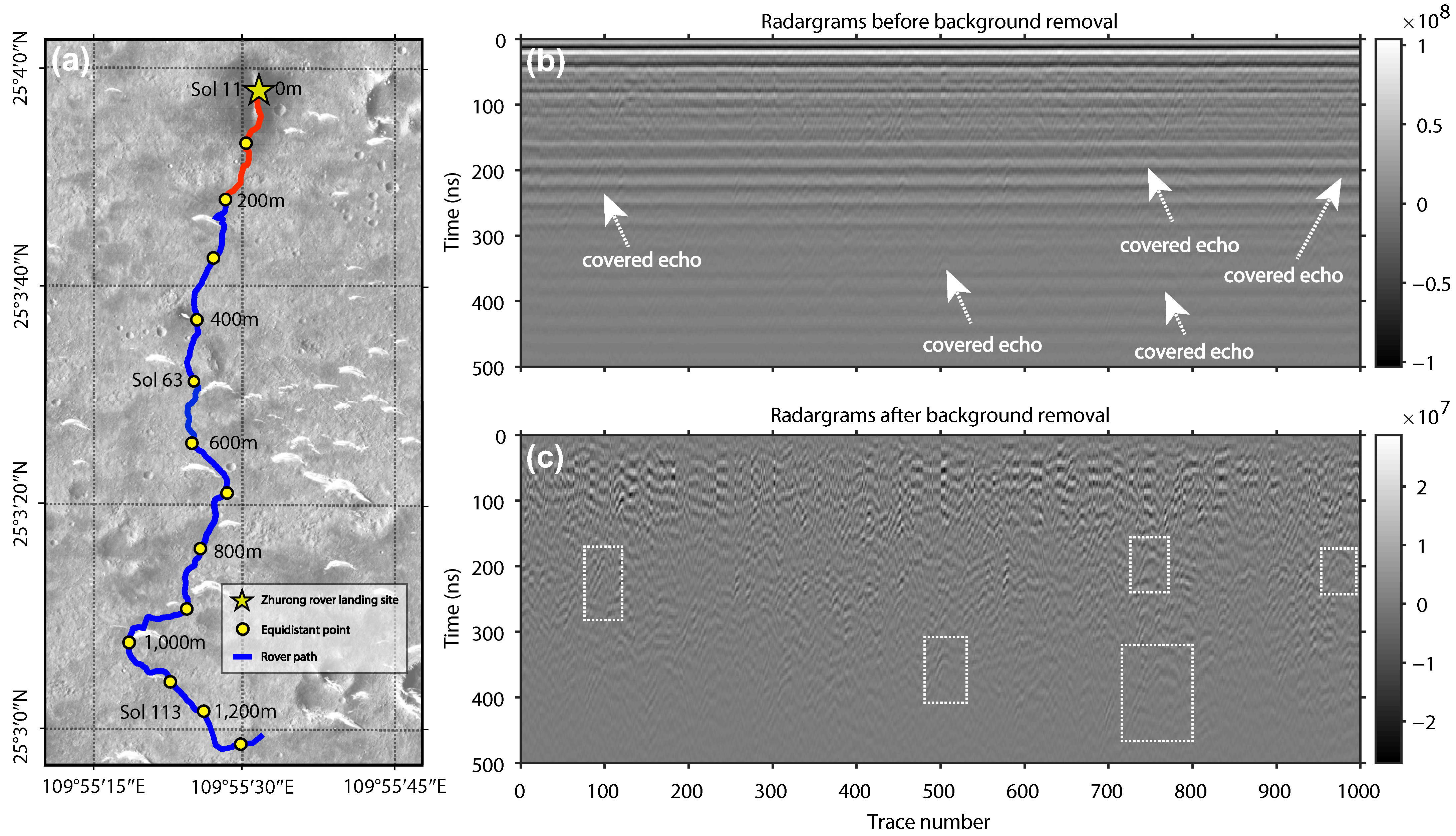
4.2. Mars Rover Data Analysis

The 2C-level RoPeR data were published by raising the frequency from the recorded intermediate frequency signal [35]. The landing site of the Zhurong rover is marked with the red star in Figure 21a. The moving distance is more than 1 km in 113 solar days. Figure 21b provides the low-frequency channel radargram of the first 200 m after LFMCW impulse compression, self-test trance removal, tracing space regularization, direct current shift removal, and time zero correction [13]. The displayed image contains only 1000 trances with a horizontal sampling interval ${\Delta }_r=0.25$ m. The displayed time length is 500 ns. Similar to the numerical simulation results, the horizontal banding noise covers almost all reflected signals. Through the previous discussion, the strong-energy horizontal banding is caused mainly by airwaves, the side lobe of impulse compression, and multiples between the rover bottom and surface. Figure 21c displays the radargrams after horizontal banding noise removal. Martian soil contains numerous scattering points of different sizes, which form substantial hyperbolic reflectors. Through the analysis of kinematic and dynamic features, the hyperbolic interface in Figure 21c is generally left tilted due to the tilted antenna. The probable hyperbolic reflectors are marked with white rectangles. The deeper scattering bodies show an imprint on more receivers with respect to offset increases. According to our theoretical analysis and numerical modeling, some of those tilted hyperbolic images might actually be caused by inclined antennas rather than subsurface geological structures. Because the RoPeR is sensitive to left-tilted structures, left-tilted interfaces are more common except for the hyperbolic. The illumination of a tilted antenna varies for different structures. During the subsequent interpretation process, these phenomena need to be analyzed to avoid misinterpretation.

According to the full-scale radargram in Figure 21c, it can be challenging to observe the scattering hyperbolas clearly. Local radargrams are cropped to allow for clearer observations of the asymmetric hyperbola characteristics (Figure 22). The five cropped local GPR images correspond to the positions marked by the rectangles in Figure 21c. The selected typical scattering hyperbolas exhibit a strong energy on the left branch and a weaker energy on the right branch. The results from the Mars field measurements provide validation of our proposed hypothesis.

The locally enlarged images of typical hyperbolic scattering patterns exhibit the clear directional characteristics of radar echoes. The numerous scattering points on the subsurface are not quantitatively evaluated. The radar images were separated using a 2D directional filter. The data analysis is based on the first 300 traces. The separated echoes show that the left-inclined radar echoes have slightly stronger energy in Figure 23a. The right-inclined radar echoes are weaker in energy in Figure 23b. The power ratio between the two types of echoes is given by $R=r_l^2/r_r^2=1.33$.

5. Discussion

In the previous section, our focus was on forward simulation using LFMCW signals and tilted antennas. The radiation characteristics of tilted antennas have implications not only for RoPeR data interpretations but also for migration processing. It has been observed that radargrams exhibit a higher reflected energy on left-inclined structures and a weaker response on right-inclined structures. Additionally, the scattering hyperbola appears to have stronger echoes on the left branch than on the right branch for scattering targets. If conventional omnidirectional antennas or horizontal dipoles are employed for migration processing, the left-inclined structure interface will inevitably appear stronger than the right-inclined interface.

Therefore, it is important to explore how to assemble the actual antenna structure into the migration process. The BP algorithm is a classical and simple migration method. A schematic illustration of the BP algorithm without antenna radiation pattern correction is shown in Figure 24a. A bistatic measurement mode (zero offsets) is considered, and the transmitter and receiver lay on the interface of a homogeneous half-space. A conventional BP algorithm assumes that the source radiates energy equally in all directions and focuses the image by stacking the energy along the hyperbolic trajectory using the following equation:

$$I(x,z)=\sum _{k=1}^N{r}_k\left(t_k(x,z)\right).$$

(6)

where $I(x,z)$ is the image intensity at position $(x,z)$, N is the number of recorded traces, $r_k\left(t_k(x,z)\right)$ is the amplitude received by k th radar position, $t_k(x,z)=2R/v$ indicates the two-way travel time from the imaging point $(x,z)$ to radar location, and R and v represent the distance and propagation velocity, respectively. This algorithm ignores the antenna radiation pattern. However, the radiation energy is not equal in all directions to real antennas. The recorded data are expressed by $r_k\left(t_k\right)=f_s\left(\theta \right)r_k^i(t_k,\theta )$, with $f_s\left(\theta \right)$ indicating the radiation pattern and $r_k^i(t_k,\theta )$ meaning the data received from an isotropic source. Because the beam width of the GPR antenna is generally wide, it is difficult to obtain $r_k^i\left(t_k\right)$ through the $f_s\left(\theta \right)$ in the data domain. We do not know which direction the echoes come from. However, the radiation patterns can be compensated in the depth domain through the BP algorithm. The RPC-BP equation is expressed as follows:

$$I_c(x,z)=\sum _{k=1}^N{f}_c\left(\theta \right)r_k\left(t_k(x,z)\right).$$

(7)

$I_c(x,z)$ is the image intensity with the radiation pattern compensation, and $f_c\left(\theta \right)$ is the correction factors corresponding to the opposite radiation patterns of the transmitter. When the GPR antenna is at position k, the correction factors can be derived from a known radiation pattern according to the angles $\theta$ between the ray paths and the horizontal direction, as illustrated in Figure 24b. Numerical simulations can be used to calculate the radiation pattern. We tested transitional BP and proposed RPC-BP algorithms based on numerical data from Figure 9 and obtained the migration images in Figure 25. The BP image with a horizontal antenna radargram shows the same energy on the left- and right-side interfaces in Figure 25a. In addition, the focused scatter point is symmetric. However, the BP image with a tilted antenna radargram has stronger energy at the left-side interface than on the opposite side. The scattering points in Figure 25b also show asymmetric characteristics. Through the proposed RPC-BP algorithm in this study, the left-side interface is reduced and the right-side impedance interface is compensated with the radiation pattern information in Figure 25c.

In this section, we have proposed a feasible solution, referred to as RPC-BP, to address the limitations of traditional BP algorithms, where the antenna radiation pattern was assembled with a BP algorithm. This approach significantly improves the illumination of right-inclined structures. Traditional BP algorithms are typically based on homogeneous medium models, directly transforming the time-domain signals into the depth domain for imaging through energy focusing. However, BP algorithm performance is poor in complex models involving non-uniform media. Finite-difference time-domain (FDTD) methods can be used to simulate the complete characteristics of electromagnetic waves, including antenna features and radiation patterns. Combining FDTD modeling of tilted antennas and reverse time migration (RTM) offers better model adaptability and broader application prospects. One practical solution is that the tilted antenna propagates the wavefield forward while an opposite-tilted antenna propagates the wavefield backward. Then, RTM imaging condition is implemented on both forward and backward wavefields. Radiation pattern compensation can be achieved in FDTD simulations.

6. Conclusions

In this study, we presented a high-accuracy forward modeling approach considering the LFMCW source, tilted antenna, and rover body effects. We analyzed the LFMCW signal, which provides high average radiation energy and resolution through impulse compression. However, it introduces side lobes and long tailings behind directly coupled waves. The RoPeR tilted antenna demonstrated a higher sensitivity to left-inclined structures, resulting in stronger reflective energy on the left side of targets. Numerical simulations revealed a tendency of rocky block reflectors leaning toward one side. The right-inclined structures reflect weak echoes. To enhance the illumination of right-inclined structures, a practical solution, called RPC-BP, was developed to obtain high-quality migration images of research areas. This method compensates for antenna radiation patterns in the depth domain and improves the imaging quality of right-inclined structures.

In addition, we conducted a laboratory experiment to verify the asymmetric scattering hyperbolas produced by tilted antennas. The observed data from the Zhurong rover showed a prominent background banding noise, which was removed to reveal a tilted hyperbola in the observed radargrams. These experimental results validate the reliability of our theoretical framework. The presence of scattering hyperbolas with specific curvatures indicates the existence of isolated rock blocks in Mars’ subsurface layer. It is important to note that artifacts, such as background banding, tilted hyperbolas, and multiples between the ground interface and rover body, are unrelated to subsurface targets but easily lead to misinterpretations.

References

1. Ernst, J.R.; Maurer, H.; Green, A.G.; Holliger, K. Full-waveform inversion of crosshole radar data based on 2-d finite-difference time-domain solutions of maxwell’s equations. IEEE Trans. Geosci. Remote Sens. 2007, 45, 2807–2828. [Google Scholar] [CrossRef]
2. Ellefsen, K.J.; Mazzella, A.T.; Horton, R.J.; McKenna, J.R. Phase and amplitude inversion of crosswell radar data. Geophysics 2011, 76, J1–J12. [Google Scholar] [CrossRef]
3. Zhong, S.; Wang, Y.; Zheng, Y. Frequency-domain wavefield reconstruction inversion of ground-penetrating radar based on sensitivity analysis. Geophys. Prospect. 2023. [Google Scholar] [CrossRef]
4. Meles, G.A.; Van Der Kruk, J.; Greenhalgh, S.A.; Ernst, J.R.; Maurer, H.; Green, A.G. A new vector waveform inversion algorithm for simultaneous updating of conductivity and permittivity parameters from combination Crosshole/Borehole-to-surface GPR data. IEEE Trans. Geosci. Remote Sens. 2010, 48, 3391–3407. [Google Scholar] [CrossRef]
5. Lavoué, F.; Brossier, R.; Métivier, L.; Garambois, S.; Virieux, J. Two-dimensional permittivity and conductivity imaging by full waveform inversion of multioffset GPR data: A frequency-domain quasi-Newton approach. Geophys. J. Int. 2014, 197, 248–268. [Google Scholar] [CrossRef] [Green Version]
6. Zhong, S.; Wang, Y.; Zheng, Y.; Chang, X. Reverse time migration of ground-penetrating radar with full wavefield decomposition based on the Hilbert transform. Geophys. Prospect. 2020, 68, 1097–1112. [Google Scholar] [CrossRef]
7. Fang, G.Y.; Zhou, B.; Ji, Y.C.; Zhang, Q.Y.; Shen, S.X.; Li, Y.X. Lunar Penetrating Radar onboard the Chang’e-3 mission. Res. Astron. Astrophys. 2014, 14, 1607–1622. [Google Scholar] [CrossRef]
8. Fa, W.; Zhu, M.H.; Liu, T.; Plescia, J.B. Regolith stratigraphy at the Chang’E-3 landing site as seen by lunar penetrating radar. Geophys. Res. Lett. 2015, 42, 10179–10187. [Google Scholar] [CrossRef]
9. Li, C.; Su, Y.; Pettinelli, E.; Xing, S.; Ding, C.; Liu, J.; Ren, X.; Lauro, S.E.; Soldovieri, F.; Zeng, X.; et al. The Moon’s farside shallow subsurface structure unveiled by Chang’E-4 Lunar Penetrating Radar. Sci. Adv. 2020, 6, eaay6898. [Google Scholar] [CrossRef] [Green Version]
10. Zhang, J.; Zhou, B.; Lin, Y.; Zhu, M.H.; Song, H.; Dong, Z.; Gao, Y.; Di, K.; Yang, W.; Lin, H.; et al. Lunar regolith and substructure at Chang’E-4 landing site in South Pole–Aitken basin. Nat. Astron. 2021, 5, 25–30. [Google Scholar] [CrossRef]
11. Hamran, S.E.; Paige, D.A.; Amundsen, H.E.; Berger, T.; Brovoll, S.; Carter, L.; Damsgård, L.; Dypvik, H.; Eide, J.; Eide, S.; et al. Radar Imager for Mars’ Subsurface Experiment—RIMFAX. Space Sci. Rev. 2020, 216, 128. [Google Scholar] [CrossRef]
12. Zhou, B.; Shen, S.X.; Lu, W.; Liu, Q.; Tang, C.J.; Li, S.D.; Fang, G.Y. The Mars rover subsurface penetrating radar onboard China’s Mars 2020 mission. Earth Planet. Phys. 2020, 4, 345–354. [Google Scholar] [CrossRef]
13. Li, C.; Zheng, Y.; Wang, X.; Zhang, J.; Wang, Y.; Chen, L.; Zhang, L.; Zhao, P.; Liu, Y.; Lv, W.; et al. Layered subsurface in Utopia Basin of Mars revealed by Zhurong rover radar. Nature 2022, 610, 308–312. [Google Scholar] [CrossRef] [PubMed]
14. Wang, Y.; Feng, X.; Zhou, H.; Dong, Z.; Liang, W.; Xue, C.; Li, X. Water ice detection research in utopia planitia based on simulation of mars rover full-polarimetric subsurface penetrating radar. Remote Sens. 2021, 13, 2685. [Google Scholar] [CrossRef]
15. Ciarletti, V.; Corbel, C.; Plettemeier, D.; Caïs, P.; Clifford, S.M.; Hamran, S.E. WISDOM GPR Designed for shallow and high-resolution sounding of the martian subsurface. Proc. IEEE 2011, 99, 824–836. [Google Scholar] [CrossRef]
16. Jol, H.M. Ground Penetrating Radar Theory and Applications; Elsevier: Amsterdam, The Netherlands, 2009. [Google Scholar] [CrossRef]
17. Lee, J.S.; Nguyen, C.; Scullion, T. A novel, compact, low-cost, impulse ground-penetrating radar for nondestructive evaluation of pavements. IEEE Trans. Instrum. Meas. 2004, 53, 1502–1509. [Google Scholar] [CrossRef]
18. Eide, S.; Casademont, T.; Aardal, Ø.L.; Hamran, S.e. Modeling FMCW Radar for Subsurface Analysis. IEEE J. Sel. Top. Appl. Earth Obs. Remote Sens. 2022, 15, 2998–3007. [Google Scholar] [CrossRef]
19. Stickley, G.F.; Noon, D.A.; Cherniakov, M.; Longstaff, I.D. Gated stepped-frequency ground penetrating radar. J. Appl. Geophys. 2000, 43, 259–269. [Google Scholar] [CrossRef]
20. Fauchard, C.; Côte, P.; Le Brusq, E.; Guillanton, E.; Dauvignac, J.Y.; Pichot, C. Step-frequency radar applied on thin road layers. J. Appl. Geophys. 2001, 47, 317–325. [Google Scholar] [CrossRef]
21. Irving, J.; Knight, R. Numerical modeling of ground-penetrating radar in 2-D using MATLAB. Comput. Geosci. 2006, 32, 1247–1258. [Google Scholar] [CrossRef]
22. Hilton, G.S.; Railton, C.J.; Ball, G.J.; Hume, A.L.; Dean, M. Finite-difference time-domain analysis of a printed dipole antenna. IEE Conf. Publ. 1995, 1, 72–75. [Google Scholar] [CrossRef]
23. Giannakis, I.; Giannopoulos, A.; Warren, C. Realistic FDTD GPR Antenna Models Optimized Using a Novel Linear/Nonlinear Full-Waveform Inversion. IEEE Trans. Geosci. Remote Sens. 2019, 57, 1768–1778. [Google Scholar] [CrossRef]
24. Lee, K.H.; Chen, C.C.; Teixeira, F.L.; Lee, R. Modeling and investigation of a geometrically complex UWB GPR antenna using FDTD. IEEE Trans. Antennas Propag. 2004, 52, 1983–1991. [Google Scholar] [CrossRef]
25. Warren, C.; Giannopoulos, A. Creating finite-difference time-domain models of commercial ground-penetrating radar antennas using Taguchi’s optimization method. Geophysics 2011, 76, G37–G47. [Google Scholar] [CrossRef]
26. Hamran, S.E.; Gjessing, D.T.; Hjelmstad, J.; Aarholt, E. Ground penetrating synthetic pulse radar: Dynamic range and modes of operation. J. Appl. Geophys. 1995, 33, 7–14. [Google Scholar] [CrossRef]
27. Hamran, S.E. Radar Performance of Ultra Wideband Waveforms. Radar Technol. 2010, 410. [Google Scholar] [CrossRef] [Green Version]
28. Tian, H.; Zhang, T.; Jia, Y.; Peng, S.; Yan, C. Zhurong: Features and mission of China’s first Mars rover. Innovation 2021, 2, 100121. [Google Scholar] [CrossRef]
29. Zhang, L.; Xu, Y.; Liu, R.; Chen, R.; Bugiolacchi, R.; Guo., R. The Dielectric Properties of Martian Regolith at the Tianwen-1 Landing Site. Geophys. Res. Lett. 2023, 50, e2022GL102207. [Google Scholar] [CrossRef]
30. Warren, C.; Giannopoulos, A.; Giannakis, I. gprMax: Open source software to simulate electromagnetic wave propagation for Ground Penetrating Radar. Comput. Phys. Commun. 2016, 209, 163–170. [Google Scholar] [CrossRef] [Green Version]
31. Warren, C.; Giannopoulos, A.; Gray, A.; Giannakis, I.; Patterson, A.; Wetter, L.; Hamrah, A. A CUDA-based GPU engine for gprMax: Open source FDTD electromagnetic simulation software. Comput. Phys. Commun. 2019, 237, 208–218. [Google Scholar] [CrossRef]
32. Li, C.; Xing, S.; Lauro, S.E.; Su, Y.; Dai, S.; Feng, J.; Cosciotti, B.; Di Paolo, F.; Mattei, E.; Xiao, Y.; et al. Pitfalls in GPR Data Interpretation: False Reflectors Detected in Lunar Radar Cross Sections by Chang’e-3. IEEE Trans. Geosci. Remote Sens. 2018, 56, 1325–1335. [Google Scholar] [CrossRef]
33. Angelopoulos, M.; Redman, D.; Pollard, W.H.; Haltigin, T.W.; Dietrich, P. Lunar ground penetrating radar: Minimizing potential data artifacts caused by signal interaction with a rover body. Adv. Space Res. 2014, 54, 2059–2072. [Google Scholar] [CrossRef]
34. Radzevicius, S.J.; Guy, E.D.; Daniels, J.J. Pitfalls in GPR data interpretation: Differentiating stratigraphy and buried objects from periodic antenna and target effects. Geophys. Res. Lett. 2000, 27, 3393–3396. [Google Scholar] [CrossRef] [Green Version]
35. Tan, X.; Liu, J.; Zhang, X.; Yan, W.; Chen, W.; Ren, X.; Zuo, W.; Li, C. Design and Validation of the Scientific Data Products for China’s Tianwen-1 Mission. Space Sci. Rev. 2021, 217, 69. [Google Scholar] [CrossRef]
Figure 1. Illustration of the LFMCW signal s ( t ) and beat frequency f b . The time-delayed reflected signal is represented by r ( t ) . The signal bandwidth, ranging from f m i n to f m a x , is denoted by B. T p and T w represent the duration of frequency sweep and penetration time window, respectively.
Remotesensing 15 03423 g001
Figure 2. Time-domain LFMCW signal (a) and frequency spectrum (b) with frequency ranging from 15 to 95 MHz. (c) is the impulse compression result of LFMCW.
Remotesensing 15 03423 g002
Figure 3. Tilted monopole antenna structure for low-frequency channels. The antenna is tilted up 16 degrees compared with horizontal direction. RoPeR module is mounted in front of the Zhurong Mars rover.
Remotesensing 15 03423 g003
Figure 4. Horizontal and tilted monopole antennas. Both load and feed points are located at the extreme point of the antennas.
Remotesensing 15 03423 g004
Figure 5. Radiation patterns of horizontal and tilted antennas. (a,b) are elevation and azimuth plane patterns of horizontal antenna for frequency of 55 MHz. (c,d) are elevation and azimuth plane patterns of tilted antenna. The maximal radiation directions of horizontal and tilted antennas are 180 ° and 164 ° in (a,c), respectively.
Remotesensing 15 03423 g005
Figure 6. 2D snapshots of horizontal (a) and tilted (b) antennas at y = 10 m, with apparent drag shadows caused by antenna reflection. The Ricker wavelet is transmitted by two antennas. The form of snapshots corresponds to the radiation pattern in Figure 5.
Remotesensing 15 03423 g006
Figure 7. Radiation performance of a monopole antenna varies with frequency from 15 to 95 MHz. Both VSWR (a) and S11 parameters (b) show that a quarter-wavelength antenna shows best performance at frequency f 55 Mhz.
Remotesensing 15 03423 g007
Figure 8. Impulse compression principle for LFMCW radar. (a) is the modeled synthetic data in time domain. (b) is the spectrum of received signal, in which low- and high-frequency components are filtered by a transmitting antenna. (c) is the synthetic response in time domain after impulse compression.
Remotesensing 15 03423 g008
Figure 9. Rocky block model for response tests of different antennas and excitation signals. Three rocky blocks are located at x 1 = ( 30 , 10 , 3 ) , x 2 = ( 50 , 10 , 8 ) , and x 3 = ( 70 , 10 , 13 ) , respectively. The red circle and cross represent the starting and ending points, respectively. The dashed yellow line is a moving track with a spatial sampling interval of 0.5 m in horizontal direction.
Remotesensing 15 03423 g009
Figure 10. Radargrams of the Hertzian dipole (a) and quarter-wavelength monopole (b) for Ricker wavelet excitation. The LFMCW response excited by a quarter-wavelength monopole and impulse compression results can be seen in (c,d). There is no tailing from the rocky blocks in (a). (b) shows short tailing after strong air and surface-reflected waves. Echoes from impulse compression in (d) last a long time.
Remotesensing 15 03423 g010
Figure 11. A-scan curve of the Ricker wavelet transmitted by a Hertzian dipole (a) and quarter-wavelength monopole antenna (b). The first break is marked with red arrows. (c,d) are recorded A-scan of LFMCW source and impulse compression echo, respectively. The echo is marked by red circles in (c) and two-way travel time is indicated by a red arrow in (d).
Remotesensing 15 03423 g011
Figure 12. (a,b) are the response descriptions of horizontal and tilted antennas to rocky blocks, respectively. (c,d) illustrate the mechanization of horizontal and tilted antennas to inclined interfaces, separately. The red and blue triangles indicate transmitting and receiving antennas, respectively. Details about low-frequency antennas are given in [12].
Remotesensing 15 03423 g012
Figure 13. Radargrams of horizontal (a) and tilted antennas (b) after impulse compression. The hyperbolic reflectors from three buried rocky blocks are marked by dashed red curves. Different-depth targets are used to show hyperbola characteristics.
Remotesensing 15 03423 g013
Figure 14. Three-dimensional Mars rover model with uniform meshes. There are six wheels and tilted antennas mounted on the bottom and front of the Mars rover, respectively. The top board is a solar system that powers the Mars rover.
Remotesensing 15 03423 g014
Figure 15. Radargrams considering Mars rover body influence. Impulse compression (a) and background removal (b) images exhibit rover-related artifacts following primary wave, in which artifacts mainly come from the rover bottom reflections.
Remotesensing 15 03423 g015
Figure 16. Martian subsurface model with rocky blocks of different sizes in three layers. A yellow dashed line indicates the rover’s moving path, where a red rover is the starting point and a cross is the ending point.
Remotesensing 15 03423 g016
Figure 17. Horizontal (a) and tilted (b) monopole antennas’ radargrams after background banding noise removal. The red arrows indicate the different characteristics of reflected hyperbolas for horizontal and tilted monopole antennas.
Remotesensing 15 03423 g017
Figure 18. Left-tilted (a) and right-tilted (b) echo waves decomposed by 2D directional filters. Left-inclined echoes are stronger than right-inclined echoes.
Remotesensing 15 03423 g018
Figure 19. Three-axis slide rail (a), tilted dipole antenna (b), and side view of the tested laboratory model (c). The 3D slide rail provides high-accuracy position control above the sandpit. The laboratory experiment tested both horizontally placed and tilted antennas.
Remotesensing 15 03423 g019
Figure 20. Radargrams of horizontal (a) and tilted antennas (b). Right-branch echoes are marked by dashed white circles, in which the scattered energy in (a) is higher than that in (b).
Remotesensing 15 03423 g020
Figure 21. (a) shows the Zhurong rover moving path, with a yellow star and red line indicating the Zhurong rover landing site and research area within the first 200 m. (b,c) are radargrams before and after horizontal banding noise removal. The white arrows indicate covered radar echoes from subsurface targets in (b). The white rectangles mean probable hyperbolic reflectors in (c).
Remotesensing 15 03423 g021
Figure 22. Local radargrams (ae) of five positions marked with the white rectangles in Figure 21c. All hyperbolas display unsymmetric characteristics, where the left branch is stronger than the right one.
Remotesensing 15 03423 g022
Figure 23. Left-tilted (a) and right-tilted (b) RoPeR echo waves decomposed by 2D directional filters. Left-inclined echoes are stronger than right-inclined echoes.
Remotesensing 15 03423 g023
Figure 24. Illustration of BP (a) and RPC-BP (b) algorithms considering antenna radiation patterns. RoPeR data collection confirms that position 1 observes stronger echoes, while position 2 observes weaker echoes at the specific underground target ( x , z ) , based on the radiation pattern f s ( θ ) in (a). By using the RPC-BP algorithm in (b), radar echoes at position 1 are compensated with a smaller antenna gain f c ( θ ) , and echoes at position 2 are compensated with a larger gain f c ( θ ) to effectively enhance the target ( x , z ) .
Remotesensing 15 03423 g024
Figure 25. (a,b) are BP images of horizontal and tilted antennas, respectively. (c) is a RPC-BP image using the proposed method. Block targets are indicated by dashed white circles. The left- and right-inclined interfaces have equal energy in (a), whereas they do not in (b). The tilted antenna gain is corrected in (c).
Remotesensing 15 03423 g025