Article

High-Resolution Estimation of Methane Emissions from Boreal and Pan-Arctic Wetlands Using Advanced Satellite Data

1
Department of Earth Sciences, Vrije Universiteit Amsterdam, 1081 HV Amsterdam, The Netherlands
2
Planet Planetary Data Service, Wilhelminastraat 43A, 2011 VK Haarlem, The Netherlands
3
Earth System Science Disciplinary Center, University of Maryland, College Park, MD 20740, USA
4
Biospheric Sciences Laboratory, NASA Goddard Space Center, Greenbelt, MD 20771, USA
5
SRON Netherlands Institute for Space Research, 2333 CA Leiden, The Netherlands
*
Author to whom correspondence should be addressed.
Remote Sens. 2023, 15(13), 3433; https://doi.org/10.3390/rs15133433
Submission received: 4 May 2023 / Revised: 1 July 2023 / Accepted: 5 July 2023 / Published: 6 July 2023
(This article belongs to the Section Biogeosciences Remote Sensing)

Abstract

:
This paper investigates the use of soil moisture data from satellites and a hydrological model as inputs to a simplified CH4 emission model (MeSMOD) for estimating CH4 emissions from boreal and pan-Arctic regions between 2015 and 2021. MeSMOD is calibrated using FLUXNET—CH4 sites and the predictive performance is evaluated using several metrics, including the Nash-Sutcliffe efficiency (NSE). Using satellite soil moisture with 100 m resolution, MeSMOD has the highest performance (NSE = 0.63) compared with using satellite soil moisture of 10 km and hydrological model soil moisture of 10 km and 50 km (NSE = 0.59, 0.56, and 0.53, respectively) against site-level CH4 flux. This study has upscaled the estimates to the pan-Arctic region using MeSMOD, resulting in comparable mean annual estimates of CH4 emissions using satellite soil moisture of 10 km (33 Tg CH4 yr−1) and hydrological model soil moisture of 10 km (39 Tg CH4 yr−1) compared with previous studies using random forest technique for upscaling (29.5 Tg CH4 yr−1), LPJ-wsl process model (30 Tg CH4 yr−1), and CH4 CAMS inversion (34 Tg CH4 yr−1). MeSMOD has also accurately captured the high methane emissions observed by LPJ-wsl and CAMS in 2016 and 2020 and effectively caught the interannual variability of CH4 emissions from 2015 to 2021. The study emphasizes the importance of using high-resolution satellite soil moisture data for accurate estimation of CH4 emissions from wetlands, as these data directly reflect soil moisture conditions and lead to more reliable estimates. The approach adopted in this study helps to reduce errors and improve our understanding of wetlands’ role in CH4 emissions, ultimately reducing uncertainties in global CH4 budgets.

1. Introduction

Wetland ecosystems, despite covering only about 8% of the Earth’s total land area, have a significant impact on the global climate. These ecosystems accumulate a substantial proportion of the soil organic carbon (SOC), estimated to be between 29–45%. Wetlands are defined as ecosystems characterized by intermittently or permanently water-saturated soils, including peatlands (such as bogs and fens), mineral soil wetlands (such as swamps and marshes), and seasonal or permanent floodplains. The anoxic conditions in wetland soils impede the decay of organic matter, leading to its accumulation and the formation of significant soil carbon reservoirs. These reservoirs represent between 20% and 30% of the estimated 1500 Pg of global soil carbon [1,2,3,4].
Wetlands are known for their carbon-rich and moist environments, which provide favorable conditions for microbial activity that breaks down organic matter under anaerobic conditions, leading to the production of methane (CH4) [5]. In fact, wetlands are the largest natural source of atmospheric CH4, contributing to roughly one-third of total natural and anthropogenic CH4 emissions [6]. CH4 is a major anthropogenic greenhouse gas that has significant warming potential after carbon dioxide (CO2) [7], contributing to 16–25% of atmospheric warming [8]. Natural wetlands are responsible for about 20–40% of the total global CH4 emissions, making them the primary contributor to the natural CH4 budget, which is estimated to be around 145 (100-183)Tg CH4 yr−1 [5]. However, there are significant discrepancies in the estimates of CH4 emissions from wetlands, which arise from uncertainties in their spatial distribution and the mechanisms that control the balance between microbial production and oxidation of CH4. These discrepancies are evident in the inconsistencies between top-down and bottom-up techniques used for CH4 emission estimates [9,10].
There is still significant uncertainty regarding the primary drivers of temporal variations in the global growth rate of atmospheric methane CH4 [5]. This uncertainty leads to a large amount of ambiguity in climate projections due to the significant changes in growth rate since 2006 [11,12]. Although climate projections focus primarily on anthropogenic emissions, natural emissions of CH4 play a crucial role as they contribute to a significant fraction of growth rate uncertainty [5]. This is because the response of these emissions to changing climatological conditions on a wide range of temporal and spatial scales is not well understood. According to Zhang et al. [6], wetland emissions of CH4 are expected to increase at a faster rate than anthropogenic CH4 emissions in the 21st century under the RCP2.6 scenario. This is due to the increasing global wetland CH4 emissions that are sensitive to temperature changes and changes in global wetland areas.
There have been several studies demonstrating that wetland CH4 emissions are influenced by both temperature and moisture levels [13,14,15]. In terrestrial ecosystems, soil moisture (SM) is recognized as a significant factor controlling carbon fluxes, including CH4 fluxes [16,17,18]. Therefore, it is crucial to investigate the spatiotemporal distribution of SM and its effects on terrestrial carbon fluxes, particularly CH4, to gain a better understanding of these processes.
The spatiotemporal distribution of soil moisture (SM) is highly uncertain due to its considerable spatial heterogeneity, which poses a significant challenge to researchers attempting to understand its impact on terrestrial carbon fluxes [17,19]. Hydrological models, which utilize meteorological data from observations or atmospheric reanalysis to simulate SM, are commonly used to estimate SM [20]. However, significant differences in SM estimates among hydrological models using the same forcing data have been observed [21]. The level of agreement among various hydrological model SM outputs is strongly influenced by factors such as hydrology parameterization, soil texture [22], model structure, and external forcing from meteorological datasets [17]. Several studies have employed predictive models to investigate the impact of SM on CH4 fluxes [16,18,21,23]. These studies have indicated that the influence of SM on CH4 fluxes is uncertain and biased [24,25,26]. Vainio et al. [27] used the random forest technique to upscale SM measurements and reported that the spatial variability of CH4 fluxes is primarily governed by SM. Vainio et al. [27] also suggested that temporal variation in SM significantly affects observed hotspots of CH4 emissions. Treat et al. [28,29] recommended high spatial and temporal resolution monitoring of SM to accurately capture temporal variations in CH4 fluxes and avoid underestimation.
Albuhaisi et al. [30] investigated the impact of model resolution on methane emissions from wetlands in the Fennoscandinavian Peninsula. They found that resolution played a significant role in wetland emissions, with a positive correlation between soil carbon and moisture. However, uncertainties persisted due to challenges in accurately representing wetland areas and the varying relationship between soil moisture and carbon availability. Albuhaisi et al. [30] emphasized the importance of increasing model resolution to improve the accuracy of global wetland models.
Various global satellite-based soil moisture (SM) datasets have become accessible in the past decade through open-source platforms or private companies [31,32,33,34,35,36,37,38]. These datasets are derived from missions such as the European Space Agency’s Soil Moisture Ocean Salinity (SMOS) [39], NASA’s Soil Moisture Active Passive ((SMAP) [40]), and the European Space Agency Sentinel-1 [41], which were specifically designed to measure SM. Beck et al. [42] conducted an assessment of different satellite and model-based SM products and found that SMAP outperformed other datasets when compared with in situ SM measurements. Zhang et al. [17] assimilated SMAP SM data into a terrestrial carbon cycle model and found that it helped reduce uncertainty in carbon flux estimates. However, SMAP SM data has a relatively coarse resolution. To address this limitation, the current study utilizes high-resolution SM datasets obtained from Planet (formerly Van der Sat) to examine whether modeling wetland CH4 fluxes can be improved by using higher-resolution SM data.
The study incorporates daily satellite SM data at 100 m and 9 km resolution to simulate CH4 fluxes from wetlands. Additionally, data from the hydrological model PCR-GLOBWB [20] are used at 5 arcminutes and 30 arcminutes resolution (approximately 9 km and 50 km, respectively) to compare the use of SM from satellites and models. The evaluation of CH4 fluxes is based on site observations from the FLUXNET-CH4 datasets [43]. The methane fluxes are scaled up to the circumpolar boreal and pan-Arctic region to assess the significance of the differences between these approaches.
The use of high-resolution soil moisture datasets for representing wetland moisture conditions has the potential to significantly decrease the uncertainty in CH4 emission estimates. These datasets provide crucial insights into the hydrological properties of wetlands, allowing for a better understanding of the correlation between soil moisture and CH4 emissions. By incorporating this information into a model for CH4 emissions, we can evaluate the enhancement of CH4 emission estimates for monitoring and quantification purposes, thereby reducing the overall level of uncertainties. Incorporating high-resolution soil moisture datasets can greatly reduce the uncertainty in estimating CH4 emissions from wetlands. These datasets provide valuable information on wetland hydrological characteristics, enabling a better understanding of the relationship between soil moisture and CH4 emissions. By integrating this information into a CH4 emission model, we can improve estimates for monitoring and quantification purposes, which will result in a reduction of overall uncertainties.
In this study, we assess the spatial and temporal dynamics of CH4 fluxes across the boreal and pan-Arctic circle (>50 N°). Our objective is to understand the interannual variations in CH4 fluxes and their potential contribution to the recent increase in the global CH4 growth rate. To address these questions, we focus on the following key aspects:
  • Importance of spatial resolution in soil moisture (SM) data for estimating methane fluxes from wetlands: We examine how the spatial resolution of SM data influences the accuracy of CH4 flux estimations from wetland areas.
  • Impact of spatial resolution on the simulated temporal variability of CH4: We analyze the effect of spatial resolution on capturing the local temporal variations in CH4 emissions, which helps us understand the dynamics of CH4 fluxes at different scales.
  • Assessment of remote sensing SM techniques compared with hydrological models: We assess the additional value of using remote sensing-based SM techniques compared with a hydrological model for simulating CH4 fluxes. This analysis helps us understand the potential benefits of incorporating satellite-derived SM data into improving CH4 emission estimates.
After this introduction, the study is divided into four sections. Section 2 outlines the methodology used in the study, including details on the model, study area, and datasets used. Section 3 provides a comparison of site-level data from 2015–2018 and extrapolation to the pan-Arctic domain for 2015–2021. Section 4 discusses the interpretation and significance of the results, considering limitations and comparisons with the LPJ-wsl model and CAMS inversions. Last, Section 5 summarizes the main conclusions, highlights critical uncertainties, and provides recommendations for future research.

2. Materials and Methods

2.1. Study Area and Wetland Map

The study area for this research was defined as the pan-Arctic region located north of 50°N, and the study period ranged from 2015 to 2021. The Copernicus Climate Change Service Land Cover Classification (CLCC) was used to identify wetlands at a high resolution. The CLCC provides gridded maps of land cover classification derived from satellite observations dating back to 1992 and is available at a resolution of 300 × 300 m2 globally for the year 2020 [44]. It maps the global land surface in 22 classes, including wetlands, using satellite images from sensors onboard RapidEye, Landsat, and Sentinel-2 [45].
Wetlands, bogs, and creeks were extracted from the Copernicus Land Cover Change dataset using class number 180 (Figure 1) [46]. Although the simulations spanned from 2015 to 2021, the CLCC data for the year 2020 were utilized, assuming no significant changes in wetland extent occurred during this period. The CLCC dataset can be accessed at (https://cds.climate.copernicus.eu/cdsapp#!/dataset/10.24381/cds.006f2c9a?tab=overview) (accessed on 23 November 2020).
To ensure that CH4 emissions were quantified only within wetland areas as defined by the CLCC wetland map, this map acted as a mask in the model we employed (Section 2.2). By employing this approach, we were able to focus specifically on wetland areas and obtain accurate estimations of CH4 emissions within those regions. It is important to note that the CLCC dataset used in our study was regridded from a higher resolution of 300 × 300 m2 to a coarser resolution of 0.1 × 0.1 degree.

2.2. Wetland Model Description

We utilize the Methane Simple Model (MeSMOD), which applies the CH4 emission scheme used by Gedney et al. [47], to estimate CH4 emissions for the case study area. The CH4 flux from wetlands, represented as FCH4 [g CH4 m−2 yr−1], is determined based on the values of soil temperature (Tsoil), soil moisture (SM), and soil organic carbon (SOC). Specifically, the calculation of FCH4 is carried out using the following formula:
F C H 4 = K C H 4 . S O C . S M . Q 10 T s o i l T 0 10
with SOC in [gC·m−2]) and SM in [m3·m−3]). Q10 is the sensitivity of the CH4 emission to a 10 K temperature change relative to T0 = 273.15 K. Tsoil is the average soil surface temperature in [K]. KCH4 is a calibration constant (d−1) relating the driving variables to the CH4 flux in [g.m−2.d−1]. The input data used in Equation (1) are for years from 2015 to 2018 (extended to 2021 for validation) and are described in the following sections. Note that all inputs are for the top 5 cm of the soil.
We recognize that our wetland model offers a highly simplified portrayal of the mechanisms governing CH4 emissions in wetlands. Nevertheless, our primary goal is to assess the effectiveness of high-resolution satellite SM observations, necessitating a computationally efficient approach that can be developed further using more advanced models in the future.
Prior studies have reported various Q10 values ranging from 1.7 to 16 for the temperature sensitivity of methane emissions from natural wetlands [48]. Additionally, apparent Q10 values of methane fluxes measured by eddy covariance range from 2.4 to 6.6 [49]. This wide range of values is due to the correlation of methane fluxes with temperature measured at different depths, which impacts the apparent Q10 values [49]. In this study, a Q10 of 3.1 was used, which corresponds to the estimated Q10 at 5 cm depth for a temperature range between 5 °C and 30 °C, according to the study by Rinne et al. [49]. However, using a single Q10 value can lead to significant errors when predicting the temperature response to CH4 emissions [50]. Therefore, a Q10 value of 2.0 was chosen for a temperature range below 5 °C and above 30 °C. Our comparison with flux measurements in Section 3.1 confirms that this approach provides a realistic representation of the temperature sensitivity to CH4 emissions in MeSMOD simulations.
We determine the KCH4 emission calibration factor by using daily CH4 flux measurements from group 1 sites within the study area (Table 1) for the years 2015–2018. The calibrated KCH4 is then utilized to simulate CH4 emissions for the remaining sites during the entire study period (2015–2018) as well as for the upscaling experiment from 2015 to 2021 (see Section 3.1). The purpose of this calibration is to ensure that our simulations align with the annual emissions measured at the FLUXNET—CH4 sites in group 1. CH4 flux measurements for these sites were obtained from (https://fluxnet.org/download-data/) (accessed on 12 March 2021). For the upscaling of CH4 emissions in the boreal and pan-Arctic regions, we used two SM datasets (see Section 3.2), and for each, we applied the corresponding calibrated KCH4 value.
We use the daily soil organic carbon (SOC) dataset from the Level 4 (L4) carbon product (SPL4CMDL) provided by NASA National Snow and Ice Data Center at 9 × 9 km2 resolution [51]. The SOC for the study area ranges between 1 and 13 kg·m−2. This range shows a clear distinction between wetlands and other ecosystems. The values of SOC at wetland locations range between 4 and 13 kg·m−2. The data were downloaded from (https://nsidc.org/data/spl4cmdl/versions/6) (accessed on 3 March 2021).
In Equation (1), we obtained temperature data from the daily average soil surface temperature (SST) of the first top layer (7 cm) from the European Centre for Medium-range Weather Forecasts reanalysis (ECMWF-ERA5) for the years 2015–2021. We assumed a negligible difference between the topsoil of 7 cm and 5 cm. The temperature data were downloaded from (https://www.ecmwf.int/en/forecasts/datasets/reanalysis-datasets/era5) (accessed on 2 March 2021) at a spatial resolution of 7 × 7 km2 and were then aggregated to a resolution of 0.1°.

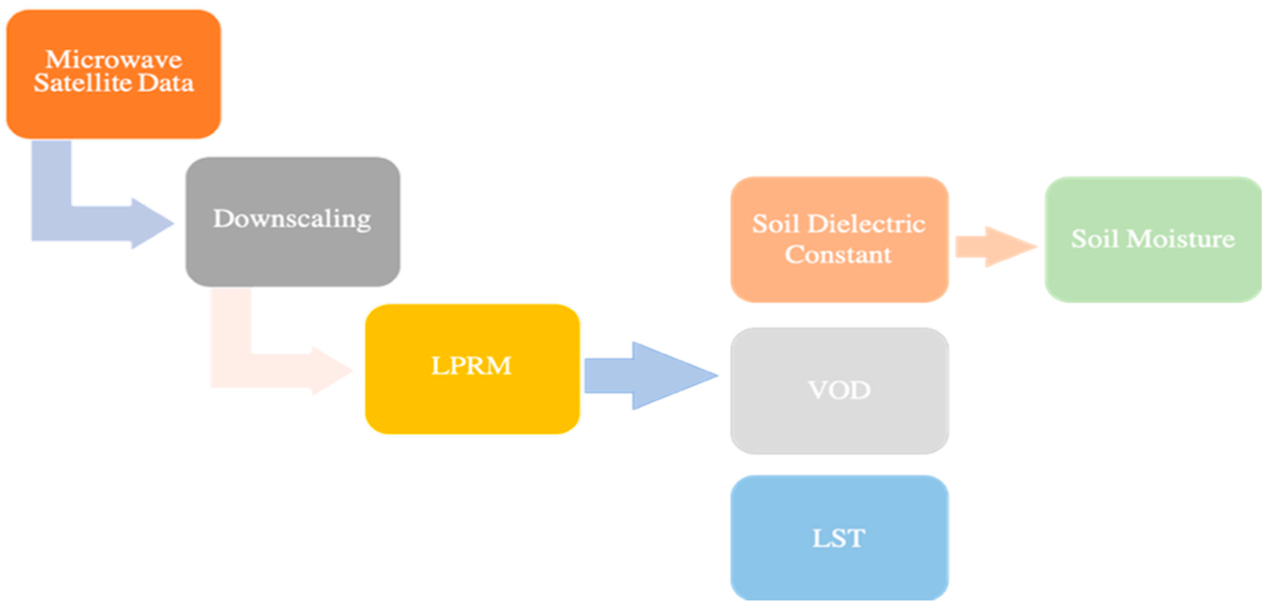
2.3. Soil Moisture Data

2.3.1. PCRaster Global Water Balance

The grid-based global hydrological model used in this study to simulate SM is called PCRaster Global Water Balance (PCR-GLOBWB), developed by the Department of Physical Geography at Utrecht University in the Netherlands [52,53]. PCR-GLOBWB comprises 5 hydrological modules—namely, meteorological forcing, land surface, groundwater, surface water routing, and irrigation and water use (Figure 2). The model simulates moisture storage in two soil layers (S1: 0–5 cm and S2: 5–30 cm) as well as water exchange between soil, atmosphere, and groundwater reservoir (Slow: 30–150 cm) for each grid cell and time step [20,52,54,55]. The modules are connected through exchange fluxes, such as precipitation, evaporation from soils, and plant transpiration. Additionally, the model accounts for 4 land cover types: tall natural vegetation, short natural vegetation, paddy-irrigated crops, and non-paddy-irrigated crops. The land cover types are proportionally aggregated to their grid cell fraction, and their effect on the exchange fluxes is considered accordingly. In this study, we focus on the top 5 cm soil layer within the unsaturated zone (Figure 2) in the land surface module, which is responsible for most CH4 production [56].
PCR-GLOBWB in our study uses daily forecast fields of precipitation, air temperature, and actual evapotranspiration from the ECMWF reanalysis data for the period 2015–2021 as its meteorological forcing. The model was forced with daily precipitation, temperature, and reference evaporation from the ECMWF ERA5 reanalysis (at 0.1° resolution) and was run at a spatial resolution of 5 arcmin (0.08°) and daily temporal resolution. The model output was subsequently aggregated to a resolution of 0.1° for this analysis.

2.3.2. Planet L-Band SM

The SM data used in this study were obtained from Planet, a global provider of satellite data, products, and services with a focus on water, soil, and crops. The company combines observations from multiple satellite sources and employs the land parameter retrieval model (LPRM) to produce remote sensing products, including SM, at a higher resolution (Figure 3) [57]. The LPRM algorithm utilizes SMAP passive microwave radiation and the relationship between the dielectric constant and SM. Planet claims that the SM data have a precision and accuracy of 0.001 m3·m−3 and 0.03 m3·m−3, respectively [58]. In this study, we utilized two resolutions of satellite SM data (100 m and 9 km) to simulate CH4 emissions for the FLUXNET—CH4 sites within the study area. The 9 km resolution was employed for upscaling over the boreal and pan-Arctic region on a daily basis.

2.4. Model Calibration and Validation Data

2.4.1. FLUXNET—CH4 Measurements

The FLUXNET—CH4 network plays a crucial role in validating the MeSMOD model. FLUXNET—CH4 encompasses a collection of ground-based flux tower sites distributed across various ecosystems globally [43,59,60]. These sites provide valuable measurements of key biophysical and biogeochemical variables, allowing for a comprehensive assessment of the model’s performance [43,59,60]. In this study, we focus on the CH4 flux measurements obtained from the FLUXNET—CH4 sites.
The CH4 flux measurements captured at the FLUXNET—CH4 sites serve as an essential benchmark for evaluating the performance of the MeSMOD model. These measurements are derived using advanced micrometeorological techniques, such as eddy covariance, which enable the direct quantification of CH4 exchange between the land surface and the atmosphere [43]. The FLUXNET—CH4 measurements offer valuable insights into the temporal dynamics and spatial variability of CH4 emissions, contributing to a robust validation of the MeSMOD model. Therefore, we utilized the daily methane flux (FCH4) data. These FCH4 measurements were included in our analysis to capture the temporal variability and dynamics of methane emissions from the selected sites. The availability of daily methane flux data further strengthens the accuracy and representativeness of the MeSMOD model calibration, validation, and parameter optimization processes.
Furthermore, it is important to note that in cases where soil moisture data were unavailable at certain FLUXNET—CH4 sites, we utilized the water table depth (WTD) as a proxy. While the primary focus of the study is on CH4 fluxes, incorporating WTD as an additional variable allows for a more comprehensive understanding of the underlying hydrological conditions that influence CH4 emissions.
For this, data from 12 wetlands, bogs, and creeks sites located within the study area (Table 1) are selected to calibrate MeSMOD (see Figure 1).

2.4.2. Model Intercomparison Data Sources

MeSMOD results have been evaluated with methane surface fluxes from the atmospheric greenhouse gas reanalysis of the Copernicus Atmosphere Monitoring Service (CAMS) [61], the process-based land surface model LPJ-wsl [62], the data-driven model WetCHARTs [11], and a random forest (RF) neural network based on eddy covariance measurements [63].
CAMS is a global atmospheric composition monitoring system that assimilates various satellite observations, in situ measurements, and model simulations. It incorporates data from multiple sources, including satellite retrievals of CH4 concentrations, surface-based observations of CH4, and simulations from atmospheric transport models. CAMS uses a data assimilation technique to optimize the model simulations and estimate CH4 fluxes at the Earth’s surface. CAMS inversions use LPJ-wsl wetland emissions as a priori estimate for CH4 fluxes [61]. We included CAMS as one of the validation models because it provides valuable estimates of CH4 fluxes for comparison with our MeSMOD model [61].
The dynamic global vegetation model (DGVM) LPJ-wsl [61] was forced by meteorological datasets from the Climatic Research Unit (CRU) and the MERRA2 reanalysis [17]. The LPJ-wsl CH4 model is based on the process-based dynamic global vegetation model of Lund–Potsdam–Jena (LPJ) [17]. It uses soil temperature, the soil moisture-dependent fraction of heterotrophic respiration (Rh), and inundation extent to calculate wetland CH4 emissions. The model is coupled to a topography-based hydrological model (TOPMODEL) to estimate wetland/inundation extent [17]. TOPMODEL uses meteorology from the CRU to simulate hydrologic fluxes of water, including lateral transport, such as evapotranspiration, subsurface flow, infiltration–excess overland flow, infiltration, exfiltration, and channel routing through a watershed. The outcomes for the years 2015 to 2021 are used in the evaluation of our results. These data were also used as a priori input in the CAMS greenhouse gas reanalysis.
The wetland CH4 emission and uncertainty dataset for atmospheric chemistry and transport modeling (WetCHARTs) calculates wetland emissions using four inundation extent parameterizations [11]. For our comparison, we use model results of the extended ensemble for the years 2001–2015 using the Global Lakes and Wetlands Database (GLWD [64]). We also compare our results using simulations from a study by Peltola et al. [63], who implemented a random forest (RF) machine-learning algorithm to simulate CH4 emissions from high-latitude wetlands for 2013–2014.
Random forest (RF) is a machine-learning algorithm utilized for classification or regression tasks. It involves building a large ensemble of regression trees, where each tree is trained independently using a random subset of training data. The RF model combines the predictions of individual trees by averaging them, taking advantage of ensemble averaging to reduce prediction noise. The algorithm employs bootstrap aggregation (bagging) to select random subsets of training data and, also, randomly selects predictor variables at each split node. This random selection minimizes correlations between trees and mitigates the risk of overfitting. Predictor variables can be categorical or continuous and are used to divide the data at split nodes based on specific criteria, such as true/false for categorical variables or a threshold value for continuous variables, such as temperature above or below 5 °C [63].
Peltola et al. [63] aimed to estimate CH4 emissions from northern high-latitude wetlands by converting upscaled flux densities into gridded emissions. To account for the uncertainty caused by different wetland mapping approaches, three wetland maps were utilized: PEATMAP, DYPTOP, and GLWD. PEATMAP is a recently developed static wetland map that focuses on peatlands but also includes marshes and swamps in certain northern latitude areas. It provides detailed geospatial information and has been converted into wetland fractions within 0.5° grid cells. The DYPTOP model is used to create a dynamic wetland map by aggregating peat and inundated areas, resulting in a 1° resolution map. GLWD, a widely used static wetland map with 30 arcsec resolution, serves as a reference and is aggregated to 0.5° resolution, excluding lakes, reservoirs, and rivers. By utilizing these different wetland maps, this study aimed to evaluate the impact of map choice on the estimation of northern high-latitude wetland CH4 emissions.

2.5. Model Performance Evaluation

To assist MeSMOD performance evaluation, we applied several statistical metrics: root-mean-square error (RMSE) between simulation and observations; index of agreement (AI); Nash–Sutcliffe efficiency (NSE), and Taylor diagram (TD).
RMSE is often used to measure the difference between model predictions and observations. The RMSE formula is:
RMSE = 1 n O b s i s i m i 2 n
where O b s i   and   s i m i represents daily CH4 observations and simulations respectively.
The index of agreement (IA) is a metric used to assess the accuracy of a model’s predictions, and its value ranges from 0 to 1. An IA value of 1 represents a perfect match between the model’s predictions and the observed data, while a value of 0 indicates no agreement at all [65]. The IA considers both the mean square error and the potential error and can detect both additive and proportional differences in the simulated and observed variances and means. However, like RMSE, IA is also sensitive to extreme values due to the squared differences. The equation for IA is:
IA = 1 i = 1 n ( O b s i S i m i ) 2 i = 1 n S i m i O b s ¯ + O b s i O b s ¯ 2 , 0 I A 1
where O b s ¯ represents the mean CH4 observations.
The Nash-Sutcliffe efficiency (NSE) is a statistical measure that normalizes the residual variance with respect to the measured data variance [66]. It quantifies the goodness of fit between observed and simulated data by assessing how closely they align on a 1:1 line. An NSE value of 1 indicates a perfect match between the model and observed data. Values greater than 0 suggest that the model performs better than the mean of the observed data, while values less than 0 indicate that the model performs worse than the mean of the validation data.
NSE = 1 i = 1 n ( O b s i S i m i ) 2 i = 1 n ( O b s i O b s ¯ ) 2
The Taylor diagram [67] is a commonly used statistical evaluation tool that compares the level of agreement between observed and modeled data by using three statistical measures: the Pearson correlation coefficient (r), the root-mean-square error (RMSE), and the standard deviation (SD). It provides a graphical representation of the degree of correspondence between the two datasets.

3. Results

This section presents local and regional simulations of CH4 fluxes from boreal and pan-Arctic wetlands, using different SM products to test MeSMOD and use it to investigate the spatiotemporal variation in the wetland CH4 flux. In Section 3.1 we will show that assimilating SSM into MeSMOD improves the CH4 representation at the site level. Section 3.2 presents the results of upscaling MeSMOD over the boreal and pan-Arctic region using two SM products (satellite and hydrological SM products).

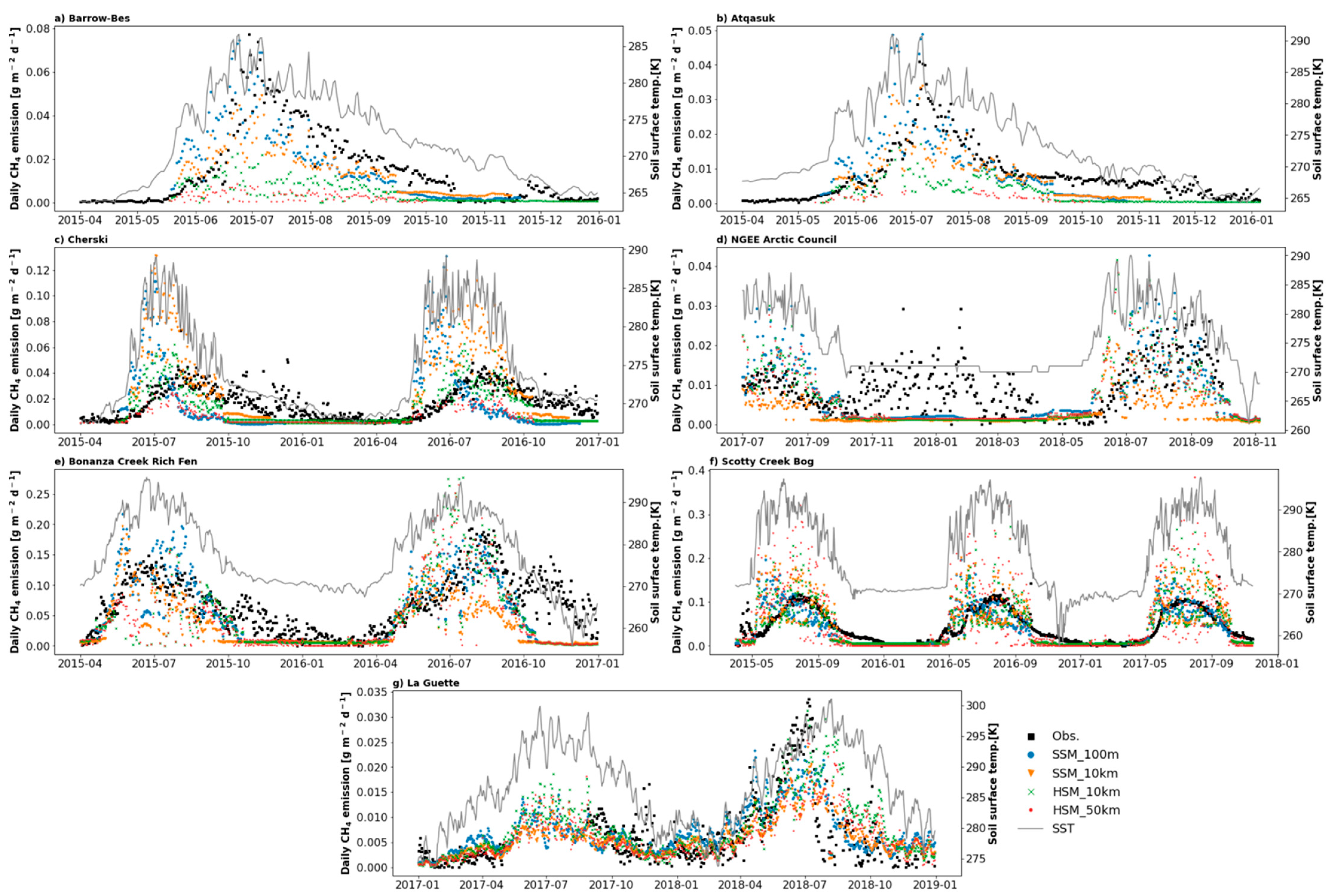
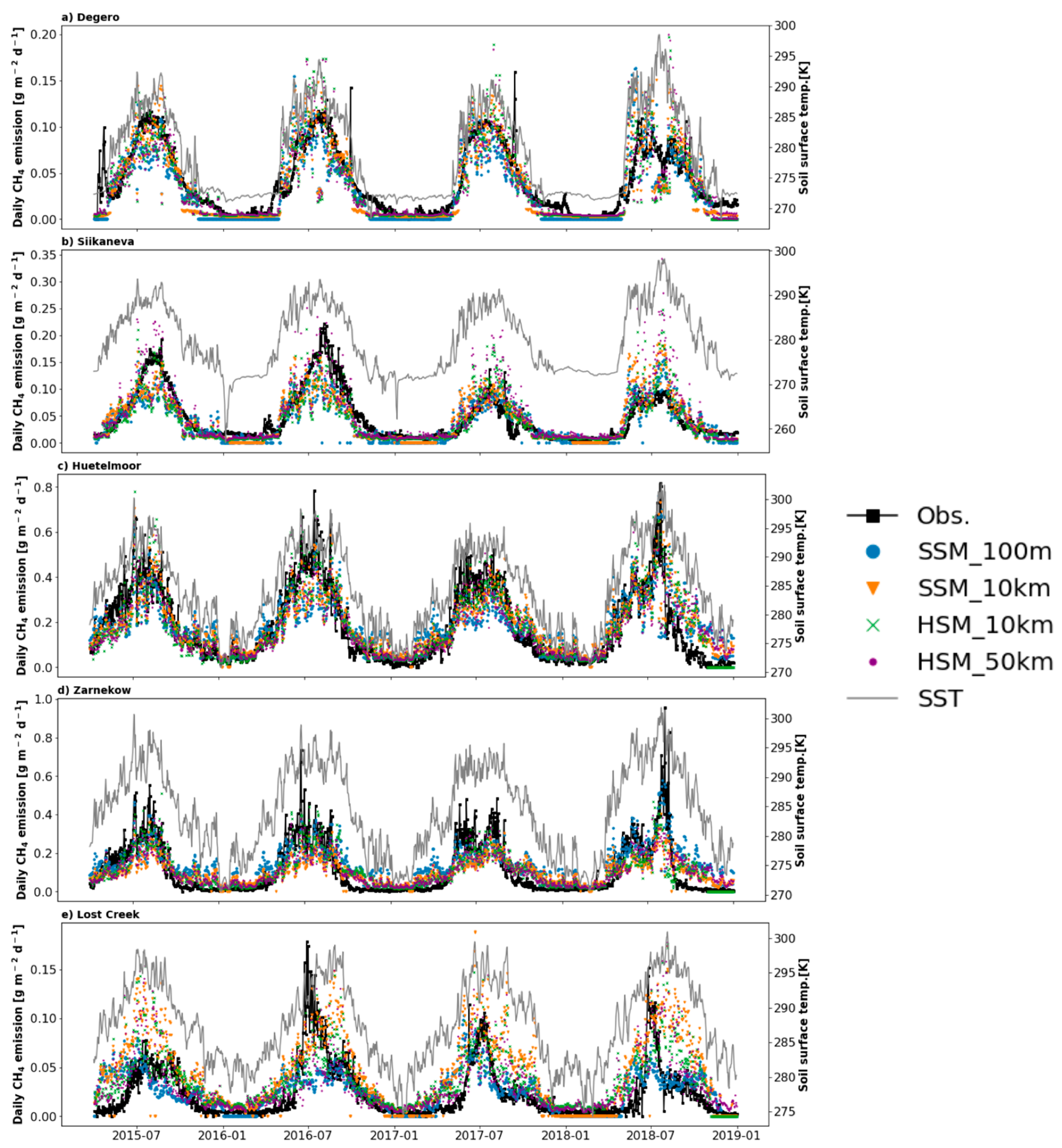
3.1. Methane Emission at Local Sites

The calibration factor KCH4 of MeSMOD (see Equation (1)) was calculated using daily CH4 flux measurements from group 1 sites within the study area for the years 2015 to 2018 (listed in Table 1). This resulted in MeSMOD simulations that matched the mean emissions of the FLUXNET—CH4 sites in group 1 during the same time frame. Subsequently, we employed this calibration value for the other sites (i.e., group 2). The KCH4 values varied (as shown in Table A2) due to the use of different soil moisture data in the study.
To test the performance of MeSMOD, CH4 flux simulations were performed for 12 measurement sites located within the study area. Figure 4 compares the use of 4 different SM datasets: Planet Satellite Soil Moisture (SSM) at 100 m and 10 km (SSM_100 m, SSM_10 km, respectively) and PCR-GLOBWB Hydrological model Soil Moisture (HSM) at 10 km and 50 km (HSM_10 km, HSM_50 km, respectively).
The results (Figure 5) show that MeSMOD is capable of reproducing the measured seasonal and interannual variability of the emissions at local sites. The seasonal pattern of the emissions closely follows the variation in temperature. Statistical methods described in Section 2.5 were used to evaluate MeSMOD (Figure 4). RMSE between MeSMOD and the validation dataset shows the best performance using SSM_100 m (RMSE = 0.05 [g·m−2 yr−1]), followed by SSM_10 km, HSM_10 km, and HSM_50 km, with slightly larger RMSE values of 0.1, 0.12, and 0.2 [g·m−2 yr−1], respectively. The index of agreement (IA) shows that SSM_100 m has the best agreement with the observations compared with SSM_10 km, HSM_10 km, and HSM_50 km (IA = 0.90, 0.83, 0.82, and 0.79, respectively). The Nash-Sutcliffe efficiency (NSE) statistics show the best performance for SSM_100 m (NSE = 0.63). SSM_10 km and HSM_10 km resolution rank second (NSE = 0.59 and 0.56, respectively), followed by the HSM_50 km resolution (NSE = 0.53). A statistical summary of the differences between the MeSMOD simulations using different SM datasets compared with the validation data is presented in the Taylor diagram of Figure 4, where SSM_100 m excels over the other SM model runs.
For group 1 sites, the mean annual simulated emission (Table 2) using SSM_100 m agrees well with the mean annual flux observations. Furthermore, the model was also able to mimic the interannual variability of the emissions for group 1 sites. The SSM_10 km and HSM_10 km also show reasonable mean annual emissions compared with the observed annual emissions. The CH4 flux estimates using HSM_50 km show the lowest performance. During the nongrowing season, MeSMOD deviates from the observed fluxes; however, the contribution of those differences to annual totals is limited. The CH4 emission seasonality varies in its agreement to observations depending on the SM dataset used as shown in Figure 5. CH4 emissions using SSM_100 m resolution match best with the observation for all group 1 sites. The improved performance of the MeSMOD model using SSM_100 m resolution, as indicated by higher NSE values (See Table A1), confirms the importance of considering finer spatial resolutions in soil moisture data for a more accurate and precise estimation of CH4 emissions (see Table A1). The daily flux magnitude is modeled well at Siikaneva, Huetelmoor, Zarnekow, and Degero, whereas at Lost Creek, MeSMOD shows less agreement during May–June 2016. Here, the observed CH4 fluxes started 1 month earlier than simulations despite the temperature not peaking in that season (Figure 5).
Group 2 sites have short observation records (see Table 1). For this group, MeSMOD is less able to capture the observed interannual variability and total annual emissions (see Table A1). MeSMOD is unable to represent CH4 fluxes for reasons that might be related to extreme weather conditions (Figure A2). At La Guette in France (Figure A2), the model has difficulty simulating the emission during the mid-summer to the end of the growing season in 2018. Data for 2017 are unfortunately not available for this site.
Despite the challenges in capturing the observed interannual variability and total annual emissions for group 2 sites, it is worth noting that MeSMOD, utilizing SSM_100 m resolution, performs better for most of the sites based on the NSE criteria, as demonstrated in Table A1. This suggests, again, that the higher-resolution soil moisture data improve the model’s performance in terms of capturing temporal variations, even if challenges remain in accurately reproducing the interannual and annual emissions for this particular group.

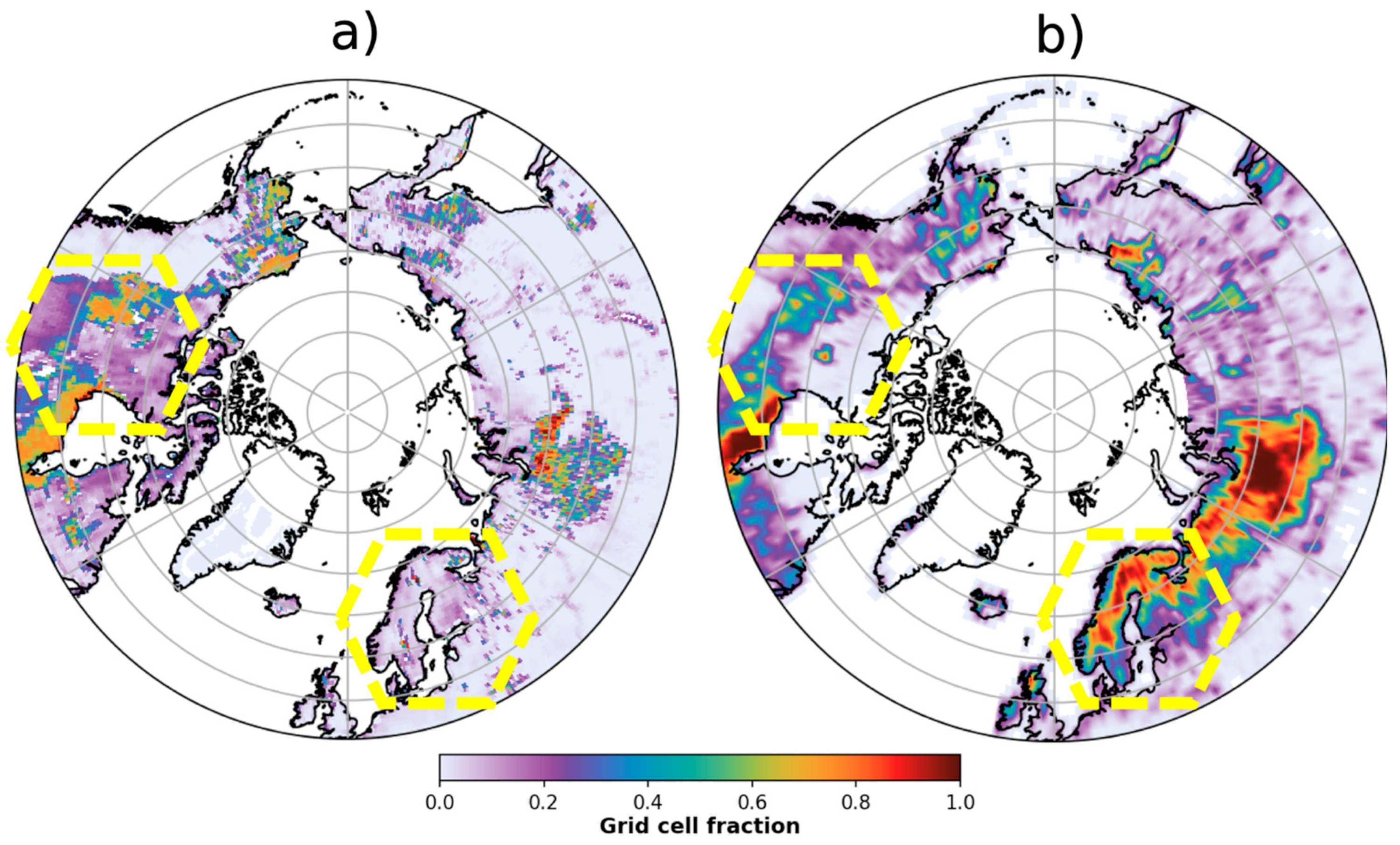
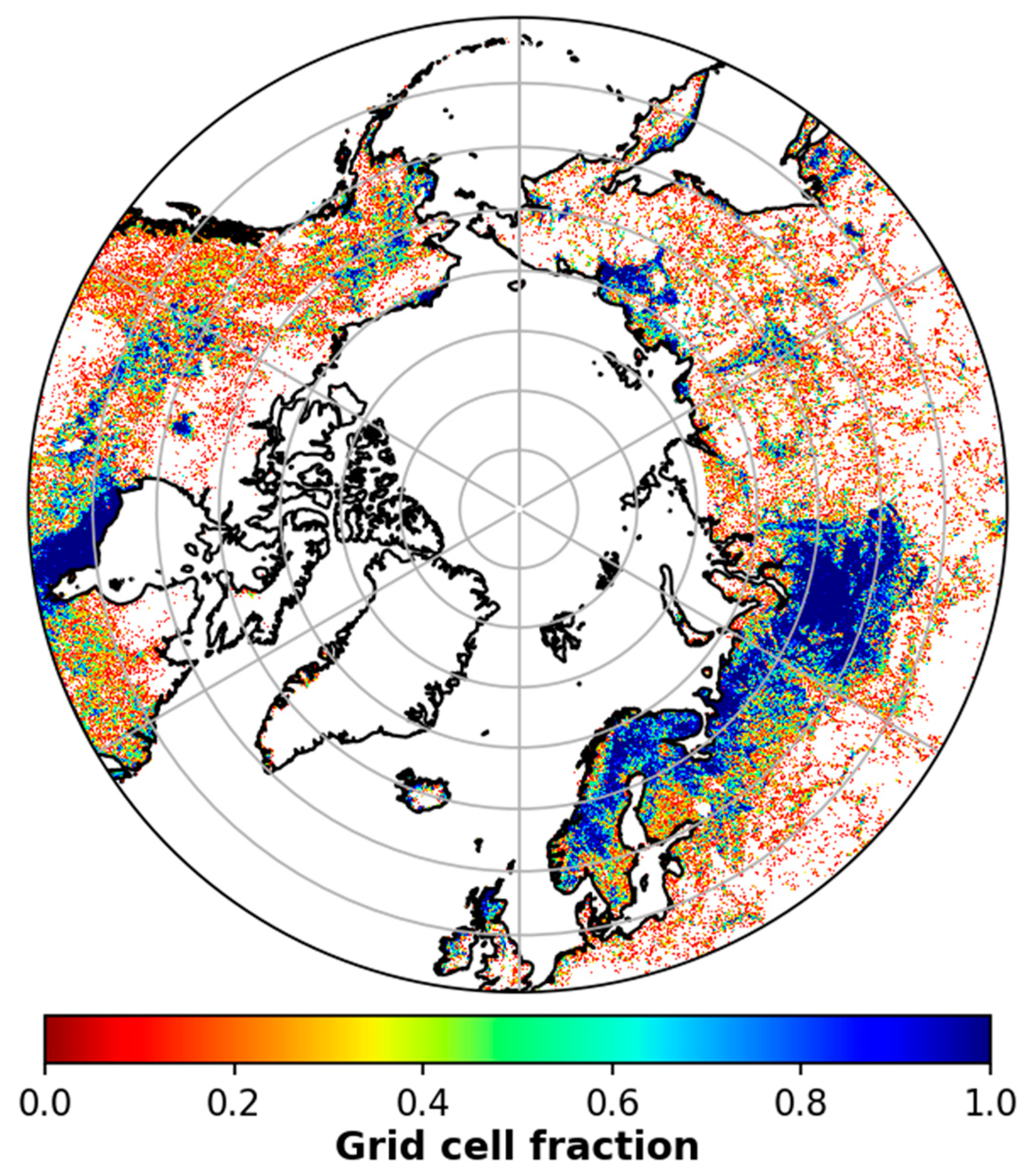
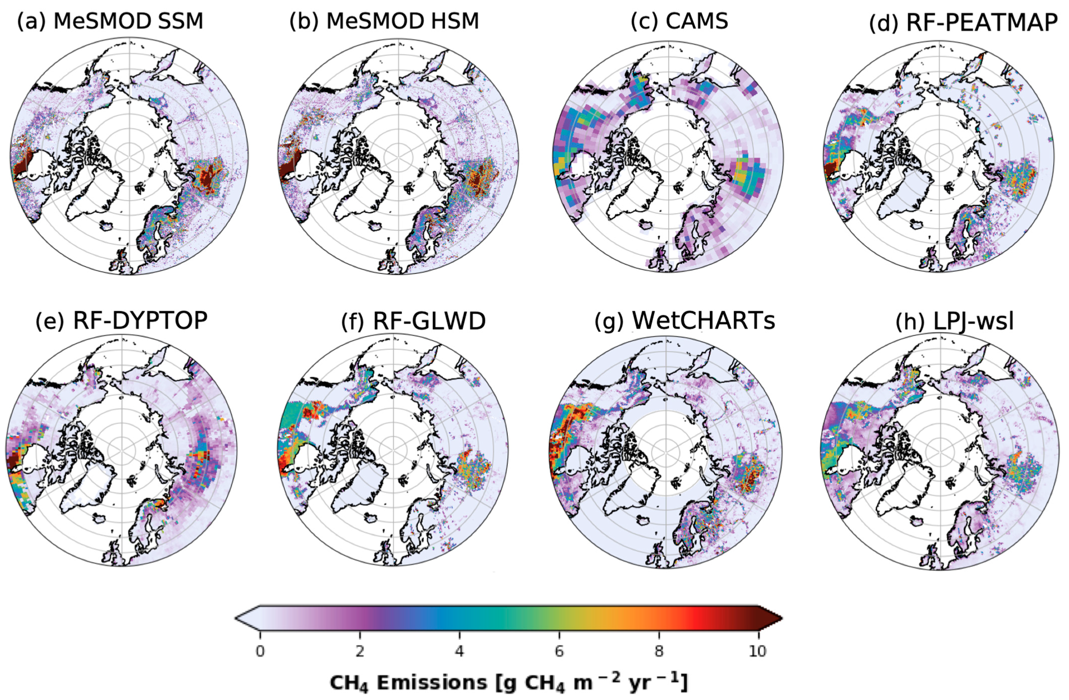
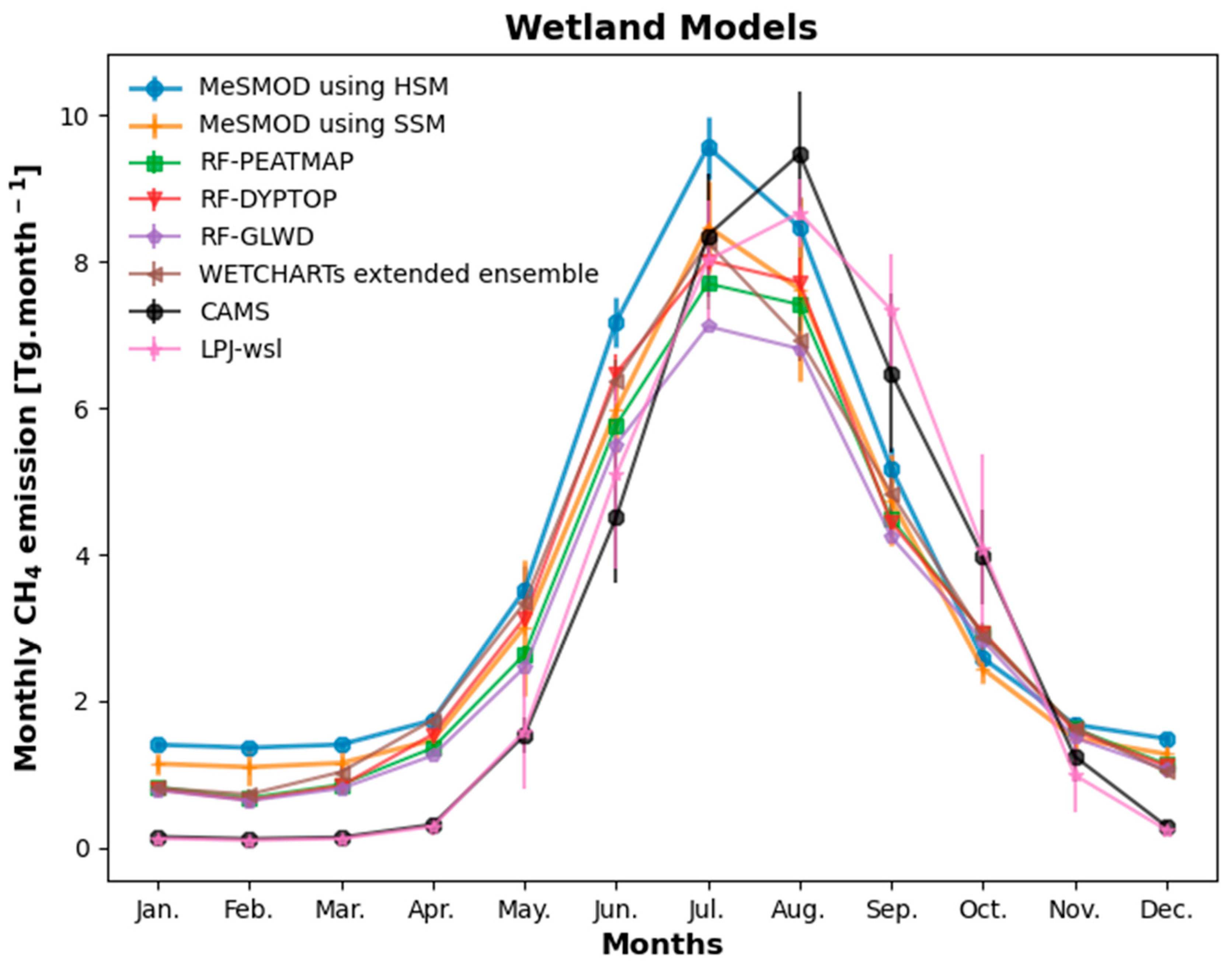
3.2. Upscaled CH4 Fluxes

The gridded input datasets (i.e., SSM and HSM at 10 km) (Section 2) are used in the MeSMOD model (hereafter MeSMOD_SSM and MeSMOD_HSM) to estimate CH4 emissions from boreal and pan-Arctic wetlands in the period between 2015 and 2021. These simulations use the data described in Section 2 and the calibration factors KCH4 from Table A2.
Results from other models, listed in Table 3, are used to evaluate the spatial emission patterns from MeSMOD. Some caution is needed in interpreting the differences between these datasets as some were only available for different time windows. Nevertheless, the comparisons are considered useful for assessing the general emission pattern from MeSMOD and its average annual emissions. The spatial patterns in Figure 6 show important differences, which is not surprising given the large spatial variability of the underlying wetland distribution maps, as reported earlier, e.g., by Peltola et al. [63]. Nevertheless, high emissions from western Canada and the West Siberian and Hudson Bay lowlands obtained from MeSMOD are in good agreement with LPJ-wsl, CAMS, WetCHARTs, RF-PEATMAP, and RF-DYPTOP. In contrast, RF-GLWD shows low emissions from the Fennoscandian peninsula (Figure 6f). These differences are largely explained by differences in the underlying wetland maps. While the wetland maps differ substantially from each other, it is not clear which ones are more accurate. Nevertheless, the comparisons indicate that the uncertainty in the upscaling of MeSMOD is driven primarily by uncertainties in wetland distribution (Figure A3). Comparing the CLCC wetland map with satellite images from Sentinel-2 and Landsat (results not shown), we found them to be in close agreement, supporting the CLCC wetland map. In addition, areas with high SOC correlate well with the CLCC wetland map (r2 = 0.41), pointing to a higher level of consistency between these maps than the spatial emission distributions in Figure 6.
The seasonality of the upscaled methane fluxes from MeSMOD and those from the reference models of Table 3 are similar (see Figure 7), with the highest CH4 emissions in July–August and the lowest in January, February, and March. In contrast, CAMS and LPJ-wsl show higher emissions in August and September. As shown in Figure 7, The MeSMOD CH4 flux magnitude agrees well with WetCHARTs and the RF models during spring and early summer (April–June), whereas LPJ-wsl and CAMS show lower fluxes in April before they start to increase sharply and reach the maximum emissions in August. During late summer and early autumn (August–October), WetCHARTs and the RF models estimate ~10% lower fluxes than MeSMOD. The upscaled MeSMOD fluxes agree with the RF models on the magnitude of nongrowing season emissions (November–March), while both are higher than WetCHARTs (+30%), LPJ-wsl, and CAMS (both +40%). The upscaled MeSMOD estimates, as well as RF models, for the nongrowing season are relatively close to each other.

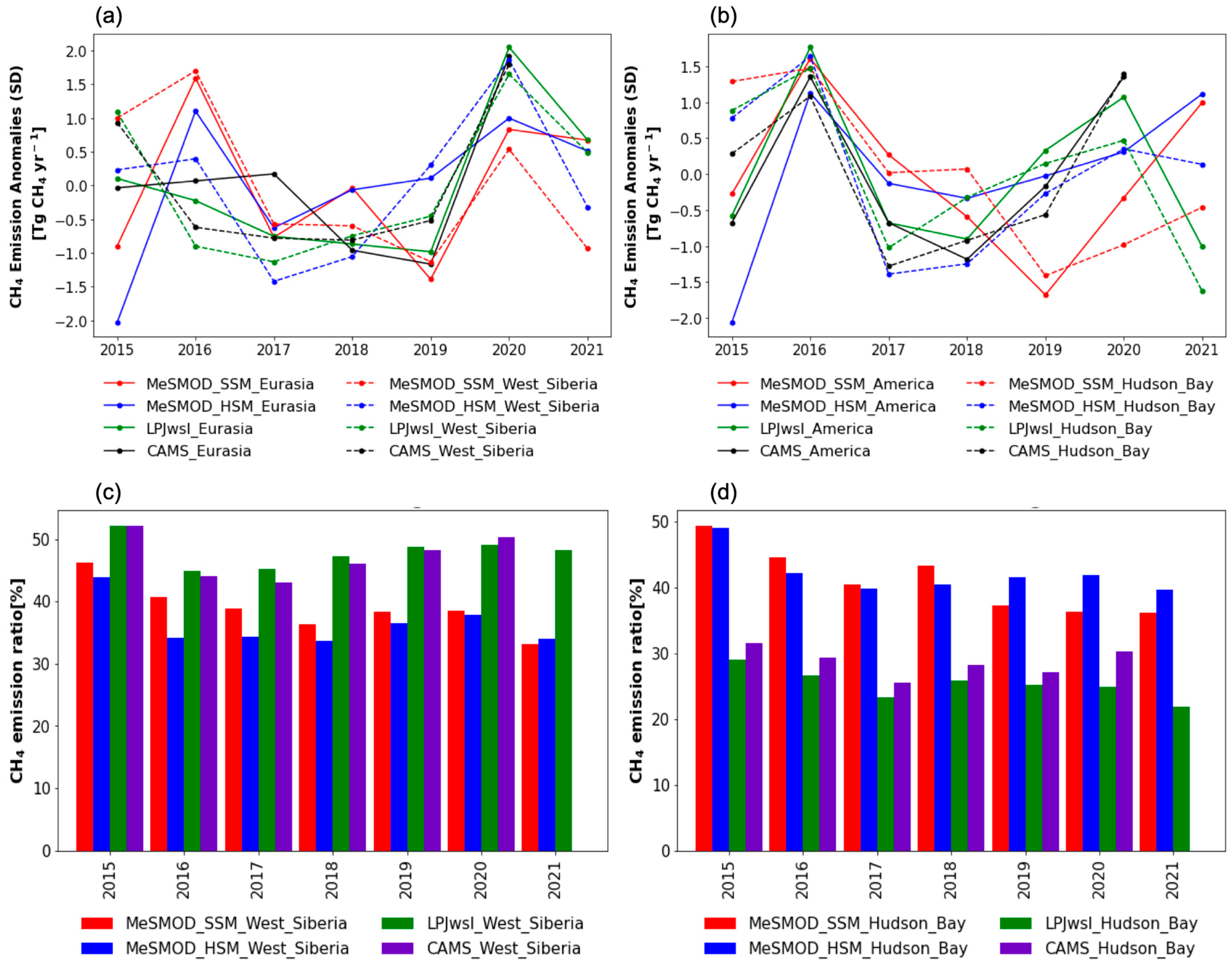
West Siberia Lowlands and Hudson Bay Wetlands

The West Siberian (WSL) and Hudson Bay (HB) lowlands are known to be the largest contributors to the pan-Arctic CH4 budget [63,69,70,71,72,73,74,75]. To further evaluate the agreement between MeSMOD upscaled fluxes with other models, we pay special attention to these regions. The upscaled MeSMOD fluxes show higher annual emissions for both subdomains than LPJ-wsl and CAMS.
For WSL (Figure 8a), the upscaled estimates of MeSMOD are within the range of variability of the LPJ-wsl process model and CAMS inversion model (Table 4). For the Eurasian domain, however, MeSMOD_SSM and MeSMOD_HSM show higher annual emissions compared with LPJ-wsl and CAMS. Comparing the spatial emission patterns, both LPJ-wsl and CAMS have fewer emissions over the Fennoscandinavian Peninsula, explaining the Eurasia difference (Figure 8c). Hence, in LPJ-wsl and CAMS, the WSL subdomain dominates the Eurasian domain emissions more than in MeSMOD_SSM and MeSMOD_HSM. Therefore, LPJ-wsl and CAMS (using LPJ-wsl as a prior estimate) might underestimate CH4 emissions from the Eurasian domain because neither accurately accounts for the contribution of the Fennoscandinavian Peninsula, which explains part of the discrepancy with the upscaled MeSMOD estimates. Hence, the upscaled CH4 emission estimates for the Eurasian domain, while large, could nevertheless be realistic. The MeSMOD_SSM- and MeSMOD_HSM-estimated WSL contributions to the Eurasian domain range between 32% and 48%, respectively, while the LPJ-wsl and CAMS estimates range between 48% and 52%, respectively.
For North America (Figure 8b), the discrepancies between upscaled MeSMOD_SSM, MeSMOD_HSM, LPJ-wsl and CAMS are reversed compared with Eurasia (see Table 4). Here MeSMOD_SSM and MeSMOD_HSM show fewer emissions compared with LPJ-wsl and CAMS, despite the estimates for the HB subdomain agreeing well with LPJ-wsl and CAMS. MeSMOD_HSM shows higher emissions than MeSMOD_SSM but still in a reasonable range (see Table 4). Both MeSMOD runs do not show high emissions in the Taiga Plains in Canada, which is again explained by the difference between the CLCC wetland map and the wetland map used by LPJ-wsl and CAMS (Table 4 and Figure 8d). It is important to mention that the lack of a sufficient number of long-term EC flux studies conducted in the HBL area makes it hard to evaluate these differences. The implementation of the CLCC wetland map in MeSMOD does not show high emissions from the Taiga Plains in Canada, which is included in the wetland map used by LPJ-wsl and CAMS explaining the smaller contribution from HB to the North American domain (LPJ-wsl 45% to 52%, CAMS 27% to 32%) compared with the MeSMOD simulations.
The difference between MeSMOD_SSM 10 km and MeSMOD_HSM 10 km is only due to SM. The mean HSM (0.32 m3.m−3) is larger than SSM (0.25 m3.m−3), explaining the larger CH4 emissions. Figure 9 shows the seasonal and interannual variability of HSM, confirming that the mean SM level is higher than that of SSM. However, the seasonal variability of SSM_10 km is stronger than that of HSM_10 km.
The annual emission anomalies in Figure 8a,b show that the estimated wetland CH4 emissions in 2016 and 2020 for North America and Eurasia are the largest over the entire period of the study. HB and WSL notably follow the same regional emission trend for MeSMOD_SSM, MeSMOD_HSM, LPJ-wsl, and CAMS. The low emissions in 2019 for North America, as well as HB, are due to a reduced SSM coverage in the period from late June to the end of July, although we filled the gap in the data for 2019 using the mean of the previous years. The anomalies for Eurasia are larger than for North America, adding up to 2.5 ± 0.5 Tg and 1 ± 0.5 Tg, respectively, with higher emissions in these regions in 2020 than in 2017 to 2019.

4. Discussion

In this paper, we assess the use of different SM datasets, at different resolutions and based on different techniques, for estimating CH4 emissions from boreal and pan-Arctic wetlands. MeSMOD was successful in simulating CH4 fluxes observed at FLUXNET—CH4 sites despite its simplicity. Our simplified approach facilitates the use of high-resolution SSM datasets for large domains, such as the pan-Arctic used in this study. Furthermore, MeSMOD is more easily adjusted and optimized in comparison to sophisticated biogeochemical models, such as LPJ-wsl used in CAMS. The performance at validation sites is sufficient for the main aim to assess the strengths and weaknesses of different SM input datasets.
Additionally, the findings presented in this study shed light on the estimation of upscaled CH4 fluxes from boreal and pan-Arctic wetlands using the MeSMOD model. The comparisons with other models and the evaluation of spatial emission patterns provide valuable insights into the performance and accuracy of MeSMOD. Furthermore, the examination of specific regions, such as the West Siberian lowlands (WSL) and Hudson Bay (HB) wetlands, allows for a detailed assessment of the agreement between MeSMOD and other models.
At the site level scale, continuous SM observations are generally not available for all of the validation sites used in the study. Therefore, we resort to the water table depth (WTD) obtained from FLUXNET—CH4 measurements, which is commonly measured to evaluate the SM datasets we used (see Figure 10). Overall, SSM_100 m shows the best agreement with WTD at most of the selected sites (r > 0.40) (see Figure 10). However, a few sites show less agreement—for example, at Siikaneva, the WTD has a lot of missing data (Figure 10f), which prevents us from calculating the correlation between the SM data we used and the WTD measured at this site. At Huetelmoor (Figure 10g), all SM products show a negative correlation with the WTD; however, SSM_100 m still compares better than the other datasets.
Due to the very sparse spatial/temporal coverage of the FLUXNET—CH4 sites (12 sites) for which sufficient data are available in our study domain, there is still a large uncertainty in the analysis that needs to be further investigated to help reduce uncertainties. Moreover, measurement sites in the HB and WSL regions, where simulated emissions are the largest, are missing [63]. The locations of flux sites are typically restricted by practical and technical limitations related to the accessibility and availability of power supplies in addition to requirements on maintenance, which are difficult to fulfill at such remote locations [63]. We agree with Peltola et al. [63] on emphasizing the importance of continued investments in sites covering all wetlands with varying plant species composition, whereas geographical representation is not necessarily as important.
For the upscaled CH4 emissions, one of the key factors influencing the spatial emission patterns is the variability of wetland distribution maps. As reported by Peltola et al. [63], there is considerable spatial variability in the distribution of wetlands, which contributes to the observed differences in emission patterns among the models. Despite these differences, it is notable that MeSMOD demonstrates good agreement with LPJ-wsl, CAMS, WetCHARTs, RF-PEATMAP, and RF-DYPTOP in terms of high emissions from western Canada, as well as the West Siberian and Hudson Bay lowlands. These regions are recognized as major contributors to the pan-Arctic CH4 budget [63,69,70,71,72,73,74,75]. On the other hand, RF-GLWD exhibits lower emissions from the Fennoscandinavian Peninsula compared with MeSMOD, primarily due to differences in the underlying wetland maps.
MeSMOD upscaled fluxes exhibit a similar seasonal pattern to the reference models. The highest CH4 emissions are observed in July–August, while the lowest emissions occur in January, February, and March. This consistency aligns with findings from previous studies conducted by Peltola et al. [63], Warwick et al. [76], and Thonat et al. [77], which have also reported peak CH4 emissions in August–September based on measurements of atmospheric CH4 mixing ratios and isotopes across the pan-Arctic. MeSMOD shows good agreement with WetCHARTs and the RF models during the spring and early summer periods. However, LPJ-wsl and CAMS display lower fluxes in April, followed by a sharp increase leading up to the peak emissions in August. In late summer and early autumn, WetCHARTs and the RF models estimate slightly lower fluxes compared with MeSMOD. Regarding nongrowing season emissions (November–March), MeSMOD estimates are relatively close to the recent model estimate by Treat et al. [29] and the RF models, while being higher than the estimates from WetCHARTs, LPJ-wsl, and CAMS.
In North America, MeSMOD_SSM and MeSMOD_HSM exhibit higher emissions compared with LPJ-wsl and CAMS. This discrepancy can be explained by the wetland map differences, specifically the inclusion of the Taiga Plains in Canada in the wetland map used by LPJ-wsl and CAMS. MeSMOD, using the CLCC wetland map, does not show high emissions from the Taiga Plains region, resulting in a smaller contribution from this region to the North American domain compared with the other models. The uncertainty in the upscaling of MeSMOD is predominantly driven by the uncertainties in wetland distribution. However, comparing the CLCC wetland map with satellite images from Sentinel-2 and Landsat reveals close agreement, supporting the accuracy of the CLCC wetland map (results not shown). Furthermore, the correlation between areas with high soil organic carbon (SOC) and the CLCC wetland map indicates a higher level of consistency between these maps compared with the spatial emission distributions. This suggests that the CLCC wetland map provides a reliable representation of wetland distribution, contributing to the overall confidence in the MeSMOD estimates.
Focusing on the West Siberian lowlands and Hudson Bay wetlands, MeSMOD demonstrates higher annual emissions compared to LPJ-wsl and CAMS. For the WSL region, the upscaled estimates of MeSMOD fall within the range of variability of the LPJ-wsl process model and CAMS inversion model. However, at the Eurasian domain level, MeSMOD_SSM and MeSMOD_HSM exhibit higher annual emissions compared with LPJ-wsl and CAMS. This discrepancy can be attributed to the fact that LPJ-wsl and CAMS overlook the contribution of the Fennoscandinavian Peninsula, leading to an underestimation of CH4 emissions from the Eurasian domain. The spatial emission patterns further highlight this difference, with LPJ-wsl and CAMS showing lower emissions over the Fennoscandinavian Peninsula compared with MeSMOD.
Examining the annual emission anomalies, it is evident that the estimated wetland CH4 emissions in 2016 and 2020 for North America and Eurasia were the highest throughout the study period. The anomalies for Eurasia and North America indicate significantly higher emissions in Eurasia and North America in 2020 compared with the years 2017 to 2019. The year 2020 was marked by a strong heat wave and early spring snowmelt, resulting from the strong stratospheric polar vortex in the preceding winter and spring. These climatological phenomena, as reported by Overland et al. [78] and Scholten et al. [79], contributed to the environmental changes observed, including polar fires. The early spring snowmelt, coupled with high temperatures, created favorable conditions for methanogenic bacteria, leading to increased CH4 emissions. The observed high emissions in Eurasia during this period align well with the reported extreme warmth in northern Eurasia during early spring to late summer in 2020 by Overland et al. [78].
Peng et al. [80] found that the increased temperatures (+0.43–0.58 °C) in 2020 led to a rise in wetland emissions from northern wetlands compared with the previous year (2019). Their study demonstrated that high precipitation over global wetlands caused an expansion of wetland areas, primarily in northern high-latitude wetlands, leading to a boost in methane production and emission. This resulted in an increase of approximately 6 ± 2.3 Tg CH4 yr−1 in CH4 emissions in 2020 compared with 2019 [80]. The results of LPJ-wsl (3 ± 2.5 Tg CH4 yr−1), CAMS (6 ± 2.1 Tg CH4 yr−1), as well as our simulations using MeSMOD_SSM (2 ± 2.1 Tg CH4 yr−1) and MeSMOD_HSM (4 ± 2.7 Tg CH4 yr−1) for the north-latitude wetlands are consistent with the results of Peng et al. [80] regarding the high emissions anomalies in 2020 relative to 2019, which also align with previous studies on wetland methane emissions in these areas [17,29,63,81,82].
The comparison between MeSMOD_SSM and MeSMOD_HSM demonstrates that the stronger seasonal variability of soil moisture is a valuable factor for explaining the seasonal variability of methane emissions in addition to temperature. The difference in CH4 flux magnitude between the two simulations can be attributed to variations in SM levels. Specifically, the higher mean SM level in HSM compared with SSM provides an explanation for the larger CH4 emissions observed in MeSMOD_HSM. This relationship between SM and CH4 emissions is further supported by the seasonal and interannual variability analysis, which confirms that SSM_10 km exhibits a more pronounced seasonal variability compared with HSM_10 km (Figure 9).
There have been many studies evaluating the usefulness of the satellite soil moisture dataset for land surface modeling. Nevertheless, our results show that the use of satellite soil moisture data at higher resolution yields realistic methane emission estimates, and therefore could provide an important independent and underused source of information that could help reduce emission uncertainties. The improved estimates of CH4 fluxes using satellite soil moisture are important to understanding and quantifying the role of terrestrial ecosystems in observed growth rate anomalies. Our findings confirm the results of Zhang et al. [17] using SMAP SM at 36 km resolution showing the capacity to capture the temporal variability of wetland CH4 emissions in regions that do not have reliable direct measurements.
High-resolution soil moisture is a valuable dataset for estimating wetland extent as it provides a better proxy than precipitation data [17]. Wetlands are characterized by high soil moisture content, representing the full hydrological balance, and soil moisture measurements at high resolution directly reflect wetland conditions, without significant mixing of signals from other water bodies, such as lakes and rivers [17]. However, it is important to acknowledge that in regions with diverse scales of rivers and lakes, some mixing of signals may still occur, and the extent of mixing in datasets such as the Planet dataset should be considered [83]. While satellite soil moisture is a useful tool for estimating wetland wetness conditions, it should be complemented with other methods, such as field measurements, to enhance accuracy.
The results of this study provide valuable insights into the estimation of upscaled CH4 fluxes from boreal and pan-Arctic wetlands using the MeSMOD model. The comparisons with other models, assessment of spatial emission patterns, and evaluation of specific regions highlight the performance and accuracy of MeSMOD. The uncertainties primarily arise from differences in wetland distribution maps, but the agreement with reference models and satellite data supports the reliability of the CLCC wetland map. The seasonality of upscaled methane fluxes is consistent with previous studies, and the findings emphasize the importance of considering the specific characteristics of different regions, such as the WSL and HB wetlands. The study also highlights the impact of climatological phenomena on CH4 emissions, particularly the significant emissions observed in 2020 due to a strong heat wave and early spring snowmelt. Overall, these findings contribute to our understanding of CH4 emissions from boreal and pan-Arctic wetlands and provide valuable insights for future research and modeling efforts.

5. Conclusions

Although numerous studies have examined the utility of different satellite soil moisture datasets for land surface modeling, this study assesses the impact of high-resolution satellite soil moisture on simulated CH4 fluxes. This study provides valuable insights into the estimation of upscaled CH4 fluxes from boreal and pan-Arctic wetlands using the MeSMOD model. The comparisons with other models, evaluation of spatial emission patterns, and examination of specific regions have shed light not only on the usefulness of high-resolution satellite soil moisture datasets but also on the performance and accuracy of the simplified MeSMOD model in capturing CH4 emissions. The results demonstrate that MeSMOD shows good agreement with reference models for regions known to be significant contributors to the pan-Arctic CH4 budget, such as the West Siberian lowlands and Hudson Bay wetlands. The seasonality at the local site and the upscaled methane fluxes aligns well with previous studies, with peak emissions occurring from July to August and low emissions from January to March. The discrepancies between models can be attributed to differences in wetland distribution maps, emphasizing the importance of accurately representing wetland extent in CH4 flux estimations. The findings contribute to our understanding of CH4 emissions from boreal and pan-Arctic wetlands, highlighting the need for improved wetland distribution maps and refined model parameterizations. Incorporating satellite imagery, remote sensing data, and ground-based observations can enhance the accuracy of wetland representation. Additionally, model parameterizations related to soil moisture should receive high priority in order to capture the complex dynamics of CH4 emissions.
Based on the findings of this study, several recommendations can be made to guide future research and modeling efforts in the field of CH4 emissions from boreal and pan-Arctic wetlands. First, there is a need to improve the accuracy and resolution of wetland mapping through the integration of satellite imagery, remote sensing data, and ground-based observations. This will enhance the representation of wetland extent and distribution, reducing uncertainties in CH4 flux estimations. Second, refining model parameterizations related to soil moisture and hydrological processes is crucial for accurate estimation of CH4 emissions. Third, continued efforts to validate CH4 flux estimates through comprehensive ground-based measurements, atmospheric monitoring networks, and isotopic analyses are essential for model evaluation and improvement. Integration of diverse datasets, including satellite observations, soil carbon measurements, and meteorological data, can provide a comprehensive understanding of the underlying processes driving CH4 emissions. Last, establishing and maintaining long-term monitoring networks across different wetland regions is crucial for capturing interannual variability, identifying trends, and assessing the impacts of climate change and land-use changes on CH4 emissions. Long-term monitoring, including hydrological measurements, can be valuable for validating the model and improving predictions of future CH4 budgets.

Author Contributions

Y.A.Y.A. performed simulations, data analysis, interpretation, and writing the paper. S.H. supervised the study. S.H., Y.v.d.V., Z.Z. and R.D.J. discussed the result. All authors have read and agreed to the published version of the manuscript.

Funding

The project is funded by the VU Amsterdam, under the carbon cycle data assimilation in the modeling of CH4 emissions from natural wetlands (project no. 2922502).

Data Availability Statement

The data presented in this study are available on request from the corresponding author.

Acknowledgments

We would like to thank the PCR-GLOBWB team for the guidance and help to run the model. We also thank our reviewers for their constructive comments and thoughtful suggestions. We thank the PIs of the FLUXNET—CH4 sites used in this study for making the datasets available to the research community. We thank Benjamin Poulter for his valuable feedback and for being able to share the data of LPJ-wsl through Zheng Zhang. We thank Arjo Segers for being able to share the data of CAMS. Thanks to SURFSara for making Snellius HPC platform available for computations via computing grant no. 17235.

Conflicts of Interest

The authors declare no conflict of interest.

Appendix A

Figure A1. (a) Detailed Taylor diagram for group 1 sites for CH4 simulations using different SM in comparison to observations. The cosine (blue) of the angle from the x-axis is the correlation coefficient between observed and simulated CH4 emission, which determines how well the simulated CH4 emission captures the daily interannual variability of the observed CH4 emission from FLUXNET—CH4 sites. The red dot on the x-axis represents observations. The radial distance from the origin (0,0) is the standard deviation. The dashed green half circles represent RMSE. The red symbols floating in the chart are the simulations. (b) Same as Figure A1a, but for group 2 sites.
Remotesensing 15 03433 g0a1aRemotesensing 15 03433 g0a1b
Figure A2. Group-2 CH4 sites emission in comparison to simulated emissions using different SM model inputs. The years vary depending on site data availability.
Remotesensing 15 03433 g0a2
Figure A3. (a) Wetland map used in LPJ-wsl simulations; (b) the CLCC wetland map used in this study. The dashed hexagons show the locations of the wetland deviation from each other.
Remotesensing 15 03433 g0a3

Appendix B

Table A1. List of NSE model performance statistical records for each site used in this study.
Site NameSSM_100 mSSM_10 kmHSM_10 kmHSM_50 km
Siikaneva0.790.75 0.72 0.70
Degero0.780.760.720.70
Huetelmoor0.670.510.460.54
Zarnekow0.780.760.760.66
Lost Creek0.450.210.130.12
Barrow-Bes 0.650.610.530.28
Atqasuk0.690.250.200.1
Cherski0.340.260.21−1.37
NGEE Arctic Council0.380.350.330.31
Bonanza Creek 0.460.250.20.16
Scotty Creek0.620.610.450.19
La Guette0.360.220.220.12
Table A2. The calibrated KCH4 factor for different soil moisture products used in MeSMOD simulations.
Soil Moisture DataSSM_100 mSSM_10 kmHSM_10 kmHSM_50 km
KCH4[d−1]0.00550.00430.00270.002

References

  1. Chen, H.; Xu, X.; Fang, C.; Li, B.; Nie, M. Differences in the Temperature Dependence of Wetland CO2 and CH4 Emissions Vary with Water Table Depth. Nat. Clim. Chang. 2021, 11, 766–771. [Google Scholar] [CrossRef]
  2. Mitsch, W.J.; Bernal, B.; Nahlik, A.M.; Mander, Ü.; Zhang, L.; Anderson, C.J.; Jørgensen, S.E.; Brix, H. Wetlands, Carbon, and Climate Change. Landsc. Ecol. 2013, 28, 583–597. [Google Scholar] [CrossRef]
  3. Nahlik, A.M.; Fennessy, M.S. Carbon Storage in US Wetlands. Nat. Commun. 2016, 7, 13835. [Google Scholar] [CrossRef] [PubMed] [Green Version]
  4. Craft, C.B.; Boon, P.I.; Burgin, A.J.; Neubauer, S.C.; Franklin, R.B.; Ardón, M.; Hopfensperger, K.N.; Lamers, L.P.M.; Gell, P. A Global Perspective on Wetland Salinization: Ecological Consequences of a Growing Threat to Freshwater Wetlands. Ecosphere 2015, 6, 1–43. [Google Scholar]
  5. Saunois, M.; Stavert, A.R.; Poulter, B.; Bousquet, P.; Canadell, J.G.; Jackson, R.B.; Raymond, P.A.; Dlugokencky, E.J.; Houweling, S. The Global Methane Budget 2000–2017. Earth Syst. Sci. Data 2020, 12, 1561–1623. [Google Scholar] [CrossRef]
  6. Zhang, Z.; Zimmermann, N.E.; Stenke, A.; Li, X.; Hodson, E.L.; Zhu, G.; Huang, C.; Poulter, B. Emerging Role of Wetland Methane Emissions in Driving 21st Century Climate Change. Proc. Natl. Acad. Sci. USA 2017, 114, 9647–9652. [Google Scholar] [CrossRef]
  7. Spahni, R.; Joos, F.; Stocker, B.D.; Steinacher, M.; Yu, Z.C. Transient Simulations of the Carbon and Nitrogen Dynamics in Northern Peatlands: From the Last Glacial Maximum to the 21st Century. Clim. Past 2013, 9, 1287–1308. [Google Scholar] [CrossRef] [Green Version]
  8. Rosentreter, J.A.; Borges, A.V.; Deemer, B.R.; Holgerson, M.A.; Liu, S.; Song, C.; Melack, J.; Raymond, P.A.; Duarte, C.M.; Allen, G.H.; et al. Half of Global Methane Emissions Come from Highly Variable Aquatic Ecosystem Sources. Nat. Geosci. 2021, 14, 225–230. [Google Scholar] [CrossRef]
  9. Kirschke, S.; Bousquet, P.; Ciais, P.; Saunois, M.; Canadell, J.G.; Dlugokencky, E.J.; Bergamaschi, P.; Bergmann, D.; Blake, D.R.; Bruhwiler, L.; et al. Three Decades of Global Methane Sources and Sinks. Nat. Geosci. 2013, 6, 813–823. [Google Scholar] [CrossRef] [Green Version]
  10. Melton, J.R.; Wania, R.; Hodson, E.L.; Poulter, B.; Ringeval, B.; Spahni, R.; Bohn, T.; Avis, C.A.; Beerling, D.J.; Chen, G.; et al. Present State of Global Wetland Extent and Wetland Methane Modelling: Conclusions from a Model Inter-Comparison Project (WETCHIMP). Biogeosciences 2013, 10, 753–788. [Google Scholar] [CrossRef] [Green Version]
  11. Anthony Bloom, A.; Bowman, W.K.; Lee, M.; Turner, J.A.; Schroeder, R.; Worden, R.J.; Weidner, R.; McDonald, C.K.; Jacob, J.D. A Global Wetland Methane Emissions and Uncertainty Dataset for Atmospheric Chemical Transport Models (WetCHARTs Version 1.0). Geosci. Model Dev. 2017, 10, 2141–2156. [Google Scholar] [CrossRef] [Green Version]
  12. IPCC. Climate Change 2007 Synthesis Report; IPCC: Geneva, Switzerland, 2007. [Google Scholar] [CrossRef]
  13. Lu, B.; Song, L.; Zang, S.; Wang, H. Warming Promotes Soil CO2 and CH4 Emissions but Decreasing Moisture Inhibits CH4 Emissions in the Permafrost Peatland of the Great Xing’an Mountains. Sci. Total Environ. 2022, 829, 154725. [Google Scholar] [CrossRef] [PubMed]
  14. Mi, J.; Li, J.; Chen, D.; Xie, Y.; Bai, Y. Predominant Control of Moisture on Soil Organic Carbon Mineralization across a Broad Range of Arid and Semiarid Ecosystems on the Mongolia Plateau. Landsc. Ecol. 2015, 30, 1683–1699. [Google Scholar] [CrossRef]
  15. Voigt, C.; Lamprecht, R.E.; Marushchak, M.E.; Lind, S.E.; Novakovskiy, A.; Aurela, M.; Martikainen, P.J.; Biasi, C. Warming of Subarctic Tundra Increases Emissions of All Three Important Greenhouse Gases–Carbon Dioxide, Methane, and Nitrous Oxide. Glob. Change Biol. 2017, 23, 3121–3138. [Google Scholar] [CrossRef]
  16. Green, J.K.; Seneviratne, S.I.; Berg, A.M.; Findell, K.L.; Hagemann, S.; Lawrence, D.M.; Gentine, P. Large Influence of Soil Moisture on Long-Term Terrestrial Carbon Uptake. Nature 2019, 565, 476–479. [Google Scholar] [CrossRef]
  17. Zhang, Z.; Chatterjee, A.; Ott, L.; Reichle, R.; Feldman, A.F.; Poulter, B. Effect of Assimilating SMAP Soil Moisture on CO2 and CH4 Fluxes through Direct Insertion in a Land Surface Model. Remote Sens. 2022, 14, 2405. [Google Scholar] [CrossRef]
  18. Dos Santos, T.; Keppel-Aleks, G.; De Roo, R.; Steiner, A.L. Can Land Surface Models Capture the Observed Soil Moisture Control of Water and Carbon Fluxes in Temperate-To-Boreal Forests? J. Geophys. Res. Biogeosci. 2021, 126, e2020JG005999. [Google Scholar] [CrossRef]
  19. Chamindu Deepagoda, T.K.K.; Smits, K.M.; Oldenburg, C.M. Effect of Subsurface Soil Moisture Variability and Atmospheric Conditions on Methane Gas Migration in Shallow Subsurface. Int. J. Greenh. Gas Control 2016, 55, 105–117. [Google Scholar] [CrossRef] [Green Version]
  20. Sutanudjaja, E.H.; van Beek, L.P.H.; Drost, N.; de Graaf, I.E.M.; de Jong, K.; Peßenteiner, S.; Straatsma, M.W.; Wada, Y.; Wanders, N.; Wisser, D.; et al. PCR-GLOBWB 2.0: A 5 Arc-Minute Global Hydrological and Water Resources Model. Geosci. Model Dev. 2018, 11, 2429–2453. [Google Scholar] [CrossRef] [Green Version]
  21. Koster, R.D.; Guo, Z.; Yang, R.; Dirmeyer, P.A.; Mitchell, K.; Puma, M.J. On the Nature of Soil Moisture in Land Surface Models. J. Clim. 2009, 22, 4322–4335. [Google Scholar] [CrossRef] [Green Version]
  22. Cosby, B.J.; Hornberger, G.M.; Clapp, R.B.; Ginn, T.R. A Statistical Exploration of the Relationships of Soil Moisture Characteristics to the Physical Properties of Soils. Water Resour. Res. 1984, 20, 682–690. [Google Scholar] [CrossRef] [Green Version]
  23. Ahlström, A.; Xia, J.; Arneth, A.; Luo, Y.; Smith, B. Importance of Vegetation Dynamics for Future Terrestrial Carbon Cycling. Environ. Res. Lett. 2015, 10, 054019, Erratum in Environ. Res. Lett. 2015, 10, 089501. [Google Scholar] [CrossRef]
  24. Zaehle, S.; Sitch, S.; Smith, B.; Hatterman, F. Effects of Parameter Uncertainties on the Modeling of Terrestrial Biosphere Dynamics. Glob. Biogeochem. Cycles 2005, 19, 1–16. [Google Scholar] [CrossRef]
  25. Knorr, W.; Heimann, M. Uncertainlies in Global Terrestrial Biosphere Modeling 1. A Comprehensive Sensitivity Analysis with a New Photosynthesis and Energy Balance Scheme. Glob. Biogeochem. Cycles 2001, 15, 207–225. [Google Scholar] [CrossRef]
  26. Booth, E.G.; Loheide, S.P. Hydroecological Model Predictions Indicate Wetter and More Diverse Soil Water Regimes and Vegetation Types Following Floodplain Restoration. J. Geophys. Res. Biogeosci. 2012, 117, 1–19. [Google Scholar] [CrossRef]
  27. Vainio, E.; Peltola, O.; Kasurinen, V.; Kieloaho, A.J.; Tuittila, E.S.; Pihlatie, M. Topography-Based Statistical Modelling Reveals High Spatial Variability and Seasonal Emission Patches in Forest Floor Methane Flux. Biogeosciences 2021, 18, 2003–2025. [Google Scholar] [CrossRef]
  28. Treat, C.C.; Jones, M.C.; Brosius, L.; Grosse, G.; Walter Anthony, K.; Frolking, S. The Role of Wetland Expansion and Successional Processes in Methane Emissions from Northern Wetlands during the Holocene. Quat. Sci. Rev. 2021, 257, 106864. [Google Scholar] [CrossRef]
  29. Treat, C.C.; Bloom, A.A.; Marushchak, M.E. Nongrowing Season Methane Emissions–A Significant Component of Annual Emissions across Northern Ecosystems. Glob. Change Biol. 2018, 24, 3331–3343. [Google Scholar] [CrossRef] [Green Version]
  30. Albuhaisi, Y.A.Y.; van der Velde, Y.; Houweling, S. The Importance of Spatial Resolution in the Modeling of Methane Emissions from Natural Wetlands. Remote Sens. 2023, 15, 2840. [Google Scholar] [CrossRef]
  31. Babaeian, E.; Sadeghi, M.; Jones, S.B.; Montzka, C.; Vereecken, H.; Tuller, M. Ground, Proximal, and Satellite Remote Sensing of Soil Moisture. Rev. Geophys. 2019, 57, 530–616. [Google Scholar] [CrossRef] [Green Version]
  32. Wagner, W.; Hahn, S.; Kidd, R.; Melzer, T.; Bartalis, Z.; Hasenauer, S.; Figa-Saldaña, J.; De Rosnay, P.; Jann, A.; Schneider, S.; et al. The ASCAT Soil Moisture Product: A Review of Its Specifications, Validation Results, and Emerging Applications. Meteorol. Z. 2013, 22, 5–33. [Google Scholar] [CrossRef] [Green Version]
  33. Parinussa, R.M.; Holmes, T.R.H.; Wanders, N.; Dorigo, W.A.; De Jeu, R.A.M. A Preliminary Study toward Consistent Soil Moisture from AMSR2. J. Hydrometeorol. 2015, 16, 932–947. [Google Scholar] [CrossRef]
  34. Kerr, Y.H.; Al-Yaari, A.; Rodriguez-Fernandez, N.; Parrens, M.; Molero, B.; Leroux, D.; Bircher, S.; Mahmoodi, A.; Mialon, A.; Richaume, P.; et al. Overview of SMOS Performance in Terms of Global Soil Moisture Monitoring after Six Years in Operation. Remote Sens. Environ. 2016, 180, 40–63. [Google Scholar] [CrossRef]
  35. Fernandez-Moran, R.; Al-Yaari, A.; Mialon, A.; Mahmoodi, A.; Al Bitar, A.; De Lannoy, G.; Rodriguez-Fernandez, N.; Lopez-Baeza, E.; Kerr, Y.; Wigneron, J.P. SMOS-IC: An Alternative SMOS Soil Moisture and Vegetation Optical Depth Product. Remote Sens. 2017, 9, 457. [Google Scholar] [CrossRef] [Green Version]
  36. Chan, S.K.; Bindlish, R.; O’Neill, P.E.; Njoku, E.; Jackson, T.; Colliander, A.; Chen, F.; Burgin, M.; Dunbar, S.; Piepmeier, J.; et al. Assessment of the SMAP Passive Soil Moisture Product. IEEE Trans. Geosci. Remote Sens. 2016, 54, 4994–5007. [Google Scholar] [CrossRef]
  37. Dorigo, W.; de Jeu, R. Satellite Soil Moisture for Advancing Our Understanding of Earth System Processes and Climate Change. Int. J. Appl. Earth Obs. Geoinf. 2016, 48, 1–4. [Google Scholar] [CrossRef]
  38. Griesfeller, A.; Lahoz, W.A.; Jeu, R.A.M.D.; Dorigo, W.; Haugen, L.E.; Svendby, T.M.; Wagner, W. Evaluation of Satellite Soil Moisture Products over Norway Using Ground-Based Observations. Int. J. Appl. Earth Obs. Geoinf. 2016, 45, 155–164. [Google Scholar] [CrossRef] [Green Version]
  39. Kerr, Y.H.; Waldteufel, P.; Wigneron, J.-P.; Delwart, S.; Cabot, F.; Boutin, J.; Escorihuela, M.-J.; Font, J.; Reul, N.; Gruhier, C.; et al. The SMOS Mission: New Tool for Monitoring Key Elements Ofthe Global Water Cycle. Proc. IEEE 2010, 98, 666–687. [Google Scholar] [CrossRef]
  40. Entekhabi, D.; Njoku, E.G.; O’Neill, P.E.; Kellogg, K.H.; Crow, W.T.; Edelstein, W.N.; Entin, J.K.; Goodman, S.D.; Jackson, T.J.; Johnson, J.; et al. The Soil Moisture Active Passive (SMAP) Mission. Proc. IEEE 2010, 98, 704–716. [Google Scholar] [CrossRef]
  41. Torres, R.; Davidson, M.; Geudtner, D. Copernicus Sentinel Mission at C- and L-Band: Current Status and Future Perspectives. In Proceedings of the IGARSS 2020—2020 IEEE International Geoscience and Remote Sensing Symposium, Online, 26 September–2 October 2020; pp. 4055–4058. [Google Scholar]
  42. Schmidt, A.J.K. The Value of Using Hydrological Datasets for Water Allocation Decisions: Earth Observations, Hydrological Models, and Seasonal Forecasts; Routledge: Abingdon-on-Thames, UK, 2019; ISBN 9780367429553. [Google Scholar]
  43. Delwiche, K.; Knox, S.H.; Malhotra, A.; Fluet-Chouinard, E.; McNicol, G.; Feron, S.; Ouyang, Z.; Papale, D.; Trotta, C.; Canfora, E.; et al. FLUXNET-CH4: A Global, Multi-Ecosystem Dataset and Analysis of Methane Seasonality from Freshwater Wetlands. Earth Syst. Sci. Data Discuss. 2021, 13, 3607–3689. [Google Scholar] [CrossRef]
  44. Copernicus. Climate Data Store 2019. Land Cover Classifcation Gridded Maps from 1992 to Present Derived from Satellite Observations. Available online: https://cds.climate.copernicus.eu/cdsapp#!/dataset/satellite-land-cover?tab=overview (accessed on 5 May 2022).
  45. Falt’an, V.; Petrovič, F.; Ot’ahel’, J.; Feranec, J.; Druga, M.; Hruška, M.; Nováček, J.; Solár, V.; Mechurová, V.; Faltan, V.; et al. Comparison of CORINE Land Cover Data with National Statistics and the Possibility to Record This Data on a Local Scale-Case Studies from Slovakia. Remote Sens. 2020, 12, 2484. [Google Scholar] [CrossRef]
  46. Defourny, P.; Lamarche, C.; Marissiaux, Q.; Carsten, B.; Martin, B.; Grit, K. Product User Guide Specification: ICDR Land Cover 2016–2020; ECMWF: Reading, UK, 2021; p. 37. [Google Scholar]
  47. Gedney, N.; Cox, P.M.; Huntingford, C. Climate Feedback from Wetland Methane Emissions. Geophys. Res. Lett. 2004, 31, 1–4. [Google Scholar] [CrossRef] [Green Version]
  48. Walter, B.P.; Heimann, M. A Process-Based, Climate-Sensitive Model to Derive Methane Emissions from Natural Wetlands: Application to Five Wetland Sites, Sensitivity to Model Parameters, and Climate. Global Biogeochem. Cycles 2000, 14, 745–765. [Google Scholar] [CrossRef] [Green Version]
  49. Rinne, J.; Tuittila, E.S.; Peltola, O.; Li, X.; Raivonen, M.; Alekseychik, P.; Haapanala, S.; Pihlatie, M.; Aurela, M.; Mammarella, I.; et al. Temporal Variation of Ecosystem Scale Methane Emission From a Boreal Fen in Relation to Temperature, Water Table Position, and Carbon Dioxide Fluxes. Global Biogeochem. Cycles 2018, 32, 1087–1106. [Google Scholar] [CrossRef] [Green Version]
  50. Wu, Q.; Ye, R.; Bridgham, S.D.; Jin, Q. Limitations of the Q10 Coefficient for Quantifying Temperature Sensitivity of Anaerobic Organic Matter Decomposition: A Modeling Based Assessment. J. Geophys. Res. Biogeosci. 2021, 126, 1–18. [Google Scholar] [CrossRef]
  51. Kimball, J.S.; Endsley, K.A.; Jones, L.A.; Kundig, T.; Reichle, R. SMAP L4 Global Daily 9 Km EASE-Grid Carbon Net Ecosystem Exchange; NSIDC: Boulder, CO, USA, 2021; Volume 6. [Google Scholar]
  52. Bosmans, J.H.C.; Van Beek, L.P.H.; Sutanudjaja, E.H.; Bierkens, M.F.P. Hydrological Impacts of Global Land Cover Change and Human Water Use. Hydrol. Earth Syst. Sci. 2017, 21, 5603–5626. [Google Scholar] [CrossRef] [Green Version]
  53. Van Beek, L.P.H.; Bierkens, M.F.P. The Global Hydrological Model PCR-GLOBWB: Conceptualization, Parameterization and Verification; Universiteit Utrecht: Utrecht, The Netherlands, 2006. [Google Scholar]
  54. Petrescu, A.M.R.; Van Beek, L.P.H.; Van Huissteden, J.; Prigent, C.; Sachs, T.; Corradi, C.A.R.; Parmentier, F.J.W.; Dolman, A.J. Modeling Regional to Global CH4 Emissions of Boreal and Arctic Wetlands. Global Biogeochem. Cycles 2010, 24, 1–12. [Google Scholar] [CrossRef] [Green Version]
  55. De Graaf, I.E.M.; Sutanudjaja, E.H.; Van Beek, L.P.H.; Bierkens, M.F.P. A High-Resolution Global-Scale Groundwater Model. Hydrol. Earth Syst. Sci. 2015, 19, 823–837. [Google Scholar] [CrossRef] [Green Version]
  56. Shao, X.; Sheng, X.; Wu, M.; Wu, H.; Ning, X. Methane Production Potential and Emission at Different Water Levels in the Restored Reed Wetland of Hangzhou Bay. PLoS ONE 2017, 12, e0185709. [Google Scholar] [CrossRef] [Green Version]
  57. De Jeu, R.A.M.; de Nijs, A.H.A.; Van Klink, M.H.W. Method and System for Improving the Resolution of Sensor. Data. Patent WO2017216186A1, 21 December 2017. [Google Scholar]
  58. De Jeu, R.A.M.; Holmes, T.R.H.; Parinussa, R.M.; Owe, M. A Spatially Coherent Global Soil Moisture Product with Improved Temporal Resolution. J. Hydrol. 2014, 516, 284–296. [Google Scholar] [CrossRef]
  59. Pastorello, G.; Trotta, C.; Canfora, E.; Chu, H.; Christianson, D.; Cheah, Y.W.; Poindexter, C.; Chen, J.; Elbashandy, A.; Humphrey, M.; et al. The FLUXNET2015 Dataset and the ONEFlux Processing Pipeline for Eddy Covariance Data. Sci. Data 2020, 7, 225. [Google Scholar] [CrossRef] [PubMed]
  60. Knox, S.H.; Jackson, R.B.; Poulter, B.; McNicol, G.; Fluet-Chouinard, E.; Zhang, Z.; Hugelius, G.; Bousquet, P.; Canadell, J.G.; Saunois, M.; et al. FluXNET-CH4 Synthesis Activity Objectives, Observations, and Future Directions. Bull. Am. Meteorol. Soc. 2019, 100, 2607–2632. [Google Scholar] [CrossRef] [Green Version]
  61. Segers, A.; Houweling, S. Description of the CH4 Inversion Production Chain; ECMWF: Reading, UK, 2019. [Google Scholar]
  62. Zhang, Z.; Zimmermann, N.E.; Kaplan, J.O.; Poulter, B. Modeling Spatiotemporal Dynamics of Global Wetlands: Comprehensive Evaluation of a New Sub-Grid TOPMODEL Parameterization and Uncertainties. Biogeosciences 2016, 13, 1387–1408. [Google Scholar] [CrossRef] [Green Version]
  63. Peltola, O.; Vesala, T.; Gao, Y.; Räty, O.; Alekseychik, P.; Aurela, M.; Chojnicki, B.; Desai, A.R.; Dolman, A.J.; Euskirchen, E.S.; et al. Monthly Gridded Data Product of Northern Wetland Methane Emissions Based on Upscaling Eddy Covariance Observations. Earth Syst. Sci. Data Discuss. 2019, 11, 1–50. [Google Scholar] [CrossRef] [Green Version]
  64. Lehner, B.; Döll, P. Development and Validation of a Global Database of Lakes, Reservoirs and Wetlands. J. Hydrol. 2004, 296, 1–22. [Google Scholar] [CrossRef]
  65. Willmott, C.J. On the Validation of Models. Phys. Geogr. 1981, 2, 184–194. [Google Scholar] [CrossRef]
  66. Nash, J.E.; Sutcliffe, J.V. River Flow Forecasting through Conceptual Models Part I—A Discussion of Principles. J. Hydrol. 1970, 10, 282–290. [Google Scholar] [CrossRef]
  67. Taylor, K.E. Summarizing Multiple Aspects of Model Performance in a Single Diagram. J. Geophys. Res. Atmos. 2001, 106, 7183–7192. [Google Scholar] [CrossRef]
  68. Parker, R.J.; Wilson, C.; Bloom, A.A.; Comyn-Platt, E.; Hayman, G.; McNorton, J.; Boesch, H.; Chipperfield, M.P. Exploring Constraints on a Wetland Methane Emission Ensemble (WetCHARTs) Using GOSAT Observations. Biogeosciences 2020, 17, 5669–5691. [Google Scholar] [CrossRef]
  69. Thompson, R.L.; Sasakawa, M.; Machida, T.; Aalto, T.; Worthy, D.; Lavric, J.V.; Myhre, C.L.; Stohl, A. Methane Fluxes in the High Northern Latitudes for 2005-2013 Estimated Using a Bayesian Atmospheric Inversion. Atmos. Chem. Phys. 2017, 17, 3553–3572. [Google Scholar] [CrossRef] [Green Version]
  70. Tan, Z.; Zhuang, Q.; Henze, D.K.; Frankenberg, C.; Dlugokencky, E.; Sweeney, C.; Turner, A.J.; Sasakawa, M.; Machida, T. Inverse Modeling of Pan-Arctic Methane Emissions at High Spatial Resolution: What Can We Learn from Assimilating Satellite Retrievals and Using Different Process-Based Wetland and Lake Biogeochemical Models? Atmos. Chem. Phys. 2016, 16, 12649–12666. [Google Scholar] [CrossRef] [Green Version]
  71. Ito, A. Methane Emission from Pan-Arctic Natural Wetlands Estimated Using a Process-Based Model, 1901–2016. Polar Sci. 2019, 21, 26–36. [Google Scholar] [CrossRef] [Green Version]
  72. Nakano, T.; Inoue, G.; Fukuda, M. Methane Consumption and Soil Respiration by a Birch Forest Soil in West Siberia. Tellus Ser. B Chem. Phys. Meteorol. 2004, 56, 223–229. [Google Scholar] [CrossRef]
  73. Zhang, Z.; Fluet-Chouinard, E.; Jensen, K.; McDonald, K.; Hugelius, G.; Gumbricht, T.; Carroll, M.; Prigent, C.; Bartsch, A.; Poulter, B. Development of the Global Dataset of Wetland Area and Dynamics for Methane Modeling (WAD2M). Earth Syst. Sci. Data 2021, 13, 2001–2023. [Google Scholar] [CrossRef]
  74. Bohn, T.J.; Melton, J.R.; Ito, A.; Kleinen, T.; Spahni, R.; Stocker, B.D.; Zhang, B.; Zhu, X.; Schroeder, R.; Glagolev, M.V.; et al. WETCHIMP-WSL: Intercomparison of Wetland Methane Emissions Models over West Siberia. Biogeosciences 2015, 12, 3321–3349. [Google Scholar] [CrossRef] [Green Version]
  75. Wecht, K.J.; Jacob, D.J.; Frankenberg, C.; Jiang, Z.; Blake, D.R. Mapping of North American Methane Emissions with High Spatial Resolution by Inversion of SCIAMACHY Satellite Data. J. Geophys. Res. 2014, 119, 7741–7756. [Google Scholar] [CrossRef]
  76. Warwick, N.J.; Cain, M.L.; Fisher, R.; France, J.L.; Lowry, D.; Michel, S.E.; Nisbet, E.G.; Vaughn, B.H.; White, J.W.C.; Pyle, J.A. Using Δ13C-CH4 and ΔD-CH4 to Constrain Arctic Methane Emissions. Atmos. Chem. Phys. 2016, 16, 14891–14908. [Google Scholar] [CrossRef] [Green Version]
  77. Thonat, T.; Saunois, M.; Bousquet, P.; Pison, I.; Tan, Z.; Zhuang, Q.; Crill, P.M.; Thornton, B.F.; Bastviken, D.; Dlugokencky, E.J.; et al. Detectability of Arctic Methane Sources at Six Sites Performing Continuous Atmospheric Measurements. Atmos. Chem. Phys. 2017, 17, 8371–8394. [Google Scholar] [CrossRef] [Green Version]
  78. Overland, J.E.; Wang, M. The 2020 Siberian Heat Wave. Int. J. Climatol. 2021, 41, E2341–E2346. [Google Scholar] [CrossRef]
  79. Scholten, R.C.; Coumou, D.; Luo, F.; Veraverbeke, S. Early Snowmelt and Polar Jet Dynamics Co-Influence Recent Extreme Siberian Fire Seasons. Science 2022, 378, 1005. [Google Scholar] [CrossRef]
  80. Peng, S.; Lin, X.; Thompson, R.L.; Xi, Y.; Liu, G.; Hauglustaine, D.; Lan, X.; Poulter, B.; Ramonet, M.; Saunois, M.; et al. Wetland Emission and Atmospheric Sink Changes Explain Methane Growth in 2020. Nature 2022, 612, 477–482. [Google Scholar] [CrossRef] [PubMed]
  81. Liu, X.; Zhuang, Q. Methane Emissions from Arctic Landscapes during 2000–2015: An Analysis with Land and Lake Biogeochemistry Models. Biogeosciences 2022, 20, 1181–1193. [Google Scholar] [CrossRef]
  82. Olefeldt, D.; Hovemyr, M.; Kuhn, M.A.; Bastviken, D.; Bohn, T.J.; Connolly, J.; Crill, P.; Euskirchen, E.S.; Finkelstein, S.A.; Genet, H.; et al. The Boreal-Arctic Wetland and Lake Dataset (BAWLD). Earth Syst. Sci. Data Discuss. 2021, 13, 5127–5149. [Google Scholar] [CrossRef]
  83. Thornton, B.F.; Wik, M.; Crill, P.M. Double-Counting Challenges the Accuracy of High-Latitude Methane Inventories. Geophys. Res. Lett. 2016, 43, 12569–12577. [Google Scholar] [CrossRef]
Figure 1. The CLCC wetland map, representing the wetland fraction in 2020, for the study domain.
Remotesensing 15 03433 g001
Figure 2. Schematic overview of the PCR-GLOBWB model. Figure adapted from Sutanudjaja et al. (2018) [20].
Remotesensing 15 03433 g002
Figure 3. Simplified flowchart of Planet data processing. Raw satellite brightness temperature data are processed via downscaling and are run through the retrieval algorithm land parameter retrieval model (LPRM) before being linked to land surface variables, such as land surface temperature (LST), vegetation optical depth (VOD), and the soil dielectric constant, which is related to soil moisture (SM). This figure is adapted from De Jeu et al. [58].
Remotesensing 15 03433 g003
Figure 4. The Taylor diagram shown in this figure is a graphical representation of the performance of different soil moisture (SM) values in simulating CH4 emissions compared with all FLUXNET—CH4 sites used in the study. The angle between the blue line and the x-axis represents the correlation coefficient (r) between the observed and simulated CH4 emissions, indicating how well the simulations capture the variability in the observations. The red dot on the x-axis represents the observations. The distance from the origin (0,0) to the red symbols in the chart represents the standard deviation, while the dashed black half circles represent the root-mean-square deviation (RMSE). The red symbols in the chart represent the simulated values. For more information about the performance of the simulations at individual sites, refer to Figure A1a,b. The value on the red quarter circle has the same standard deviation as the observations.
Remotesensing 15 03433 g004
Figure 5. Group-1 CH4 site emission measurements (black) in comparison to simulated emissions using different SM inputs for April 2015 to December 2018 and soil surface temperature (grey).
Remotesensing 15 03433 g005
Figure 6. Mean annual CH4 wetland emissions estimated by upscaling FLUXNET—CH4 EC data using (a) Planet satellite SSM 10 km (2015–2018); (b) PCR-GLOBWB hydrological HSM 10 km (2015–2018); (c) CH4 from CAMS inversion (2015–2018); (df) RF-PEATMAP, RF-DYPTOP, and RF-GLWD models using three different wetland maps (2013–2014); (g) WetCHARTs extended ensemble (mean of all models) (2001–2015); and (h) LPJ-wsl (2015–2018).
Remotesensing 15 03433 g006
Figure 7. Seasonal variation of CH4 of the upscaled MeSMOD emissions in comparison to different models covering the same study area.
Remotesensing 15 03433 g007
Figure 8. (a) HB and (b) WSL emission anomalies compared with North American and Eurasian anomalies, respectively; (c) HB and (d) WSL contribution ratio to the CH4 emission annual total budget for North America and Eurasia, respectively.
Remotesensing 15 03433 g008
Figure 9. Study area HSM_10 km and SSM_10 km mean seasonal interannual variability for the years 2015–2021.
Remotesensing 15 03433 g009
Figure 10. Monthly anomalies of the mean SM from Planet and PCR-GLOBWB in comparison to WTD expressed in units of SD.
Remotesensing 15 03433 g010
Table 1. List of sites used in this study.
Group No.No.Site IDSite NameCoordinates (Degrees)Data AvailabilityReference
LatLon2015201620172018DOI
Group 1 *1FI-SiiSiikaneva61.8324.19++++https://doi.org/10.18140/FLX/1669640
2SE-DegDegero64.1819.56++++https://doi.org/10.18140/FLX/1669659
3DE-HteHuetelmoor54.2112.18++++https://doi.org/10.18140/FLX/1669634
4DE-ZrkZarnekow53.8812.89++++https://doi.org/10.18140/FLX/1669636
5US-LosLost Creek46.08−89.98++++https://doi.org/10.18140/FLX/1669613
Group 2 **6US-BesBarrow-Bes71.28−156.6+ https://doi.org/10.18140/FLX/1669665
7US-AtqAtqasuk70.47−157.41++ https://doi.org/10.18140/FLX/1669663
8RU-CheCherski68.61161.34++ https://doi.org/10.18140/FLX/1669655
9US-NGCNGEE Arctic Council64.86−163.7 ++https://doi.org/10.18140/FLX/1669688
10US-BZFBonanza Creek64.7−148.31++ https://doi.org/10.18140/FLX/1669669
11CA-SCBScotty Creek61.31−121.3+++ https://doi.org/10.18140/FLX/1669613
12FR-LGtLa Guette47.322.28 ++https://doi.org/10.18140/FLX/1669641
* Group 1: Sites with temporal coverage of 4 years. ** Group 2: Sites with temporal coverage of less than 4 years.
Table 2. CH4 mean annual emission for the sites used in the study (2015–2018).
Site NameFlux (g CH4 yr/m2)
ObservationSSM_100 mSSM_10 kmHSM_10 kmHSM_50 km
Group 1Degero15.30 ± 0.511.61 ± 0.513.32 ± 0.514.06 ± 0.613.89 ± 0.5
Siikaneva17.52 ± 0.714.45 ± 0.516.02 ± 0.616.26 ± 0.619.69 ± 0.8
Huetelmoor67.60 ± 2.466.85 ± 2.169.69 ± 2.368.29 ± 2.364.90 ± 2.5
Zarnekow43.06 ± 1.850.42 ± 1.637.96 ± 1.241.63 ± 1.440.88 ± 1.3
Lost Creek9.12 ± 0.49.17 ± 0.3216.69 ± 0.613.68 ± 0.512.63 ± 0.6
Group 2Barrow-Bes4.05 ± 0.43.37 ± 0.342.63 ± 0.441.09 ± 0.450.35 ± 0.47
Atqasuk2.28 ± 0.191.88 ± 0.201.46 ± 0.220.73 ± 0.070.11 ± 0.01
Cherski10.77 ± 0.508.20 ± 0.7014.16 ± 0.907.87 ± 0.502.15 ± 0.17
NGEE Arctic Council4.06 ± 0.243.22 ± 0.231.51 ± 0.103.40 ± 0.203.40 ± 0.12
Bonanza Creek43.62 ± 2.133.66 ± 2.0022.76 ± 1.4027.29 ± 1.8025.58 ± 1.70
Scotty Creek43.10 ± 1.836.46 ± 1.843.35 ± 2.245.38 ± 2.252.62 ± 2.8
La Guette3.59 ± 0.235.17 ± 0.234.23 ± 0.195.71 ± 0.274.63 ± 0.21
Table 3. A list of models compared with MeSMOD, where the annual CH4 emissions represent the average value of each model, accompanied by a ± 1σ range indicating the interannual variation in the model estimates. Please note that the estimates from certain reference models may not correspond to the same time period.
ReferenceModel NameYearsAnnual Emission North of 50° N
(Tg CH4 yr−1)
Inversion ModelCopernicus Atmosphere Monitoring ServiceCAMS v21r12015 to 202034 ± 2.50
Process ModelsBloom et al. [68]WetCHARTs2001 to 201525 ± 3.70
Zhang et al. [17]LPJ-wsl2015 to 202130 ± 2.70
Flux measurement upscalingPeltola et al. [63]RF-PEATMAP2013 and 201429 (22.3–41.2)
RF-DYPTOP2013 and 201428 (21.4–39.9)
RF-GLWD2013 and 201432 (25.9–49.5)
This studyMeSMOD_SSM2015 to 202133 ± 2.30
This studyMeSMOD_HSM39 ± 2.0
Table 4. The mean seasonal emissions of MeSMOD HSM_10 km and SSM_10 km were compared with those of LPJ-wsl and CAMS for the study area, covering the years 2015–2021, with the bracketed range indicating the annual variability.
ModelNorth-AmericaEurasiaHBWSL
CAMS23.33 (21.21–26.31)16.11 (15.02–18.10)6.70 (5.63–7.87)7.64 (7.00–9.06)
LPJ-wsl17.60 (16.44–19.64)12.75 (12.06–14.18)4.45 (3.59–5.23)6.11 (5.53–6.97)
MeSMOD_SSM14.62 (12.91–16.12)17.24 (15.32–19.44)4.61 (3.71–5.55)6.69 (5.88–7.90)
MeSMOD_HSM17.24 (15.13–19.4)21.52 (17.98–23.44)6.49 (6.11–6.94)7.77 (7.00–8.79)
Disclaimer/Publisher’s Note: The statements, opinions and data contained in all publications are solely those of the individual author(s) and contributor(s) and not of MDPI and/or the editor(s). MDPI and/or the editor(s) disclaim responsibility for any injury to people or property resulting from any ideas, methods, instructions or products referred to in the content.

