Abstract
Infrared dim small target detection has received a lot of attention, because it is a crucial component of the IR search and track systems (IRST). The robust principal component analysis (RPCA) is a common detection framework, which works with poor performance with complex background edges and sparse clutters due to the inappropriate approximation of sparse items. A nonconvex constraint detection method based on the difference between the L1 and L2 (L1–L2) norm and total variation (TV) is presented. The L1–L2 norm is a more accurate sparse item approximation of L0 norm, which can achieve a better description of the sparse item to separate the target from the complex backgrounds. Then, the total variation norm is conducted on the target image to suppress the sparse clutters. The new model is solved using the alternating direction method of multipliers (ADMM) method. Then, the subproblems in the model are tackled by the difference of convex algorithm (DCA) and the Newton conjugate gradient (Newton-CG) solving L1–L2 norm and TV norm, respectively. In the experiment, we conducted experiments on multiple and single target datasets, and the proposed model outperforms the state-of-the-art (SOTA) methods in terms of background suppression and robustness to accurately detect the target. It can achieve a higher true position rate (TPR) with a low false position rate (FPR).
1. Introduction
The Infrared search and track systems (IRST), which outperform conventional radar in early-warning, precision guidance, and surveillance applications [1], rely heavily on the infrared small target detection task. On the one hand, the target, is far from the sensor, so it takes up few pixels in the IR image. Additionally, due to the same reason, the radiation attenuation of the target is serious, resulting in a low signal to noise ratio (SNR) of the target. On the other hand, the target is obscured by the intricate background and noise. As a result, it is challenging to detect dim and small targets without shape or texture information.
Decades ago, the RPCA framework was proposed for small target detection, and data optimization-based methods have received a lot of attention because of their excellent detection performance. The low rank and sparse characteristics are respectively represented by the nuclear norm and the L0 norm. The L1 norm always replaces the L0 norm as the sparse measure; however, the loose approximation may cause under punishment of the sparse item [2]. In addition, the target image will remain at the edge clutters and sparse clutters, inducing high false detection rates in the complex background.
Therefore, to obtain more accuracy and robust detection, the improvement of the sparse item was conducted. In [3], the Lp norm was considered a better approximation to the L0 norm, which can recover the sparse signals better when 0 < p < 1. For the RPCA framework, the Lp norm is supposed to become a sparser component, and, if the value of p is smaller, the solution is sparser. Thus, the nonconvex optimization of the Lp norm can achieve superior performance for the small target detection tasks. However, the setting of p makes a decisive role in the robustness of the Lp norm model. The value of p is close to 1, and the optimization results are similar to L1. When p is close to 0, the solution is much sparser. The false alarms will be high when the initial value of p is high in the complicated background, and the low value of p may cause missed detection in the uniform background. Therefore, the model based on the Lp norm is inadequate to apply in multifarious circumstances with IR small target detection tasks.
Furthermore, the SOTA methods based on matrix recovery can well achieve detection with homogenous scenes, while they are still affected by the sparse clutters, such as cloud edges, sun flash, and sea clutters. The sparse constraint is poor robustness to distinguish the target from the clutters and a high false alarm due to the heavy residual in the target image. TV norm [4] has already been applied to the yield of image denoise. Ideally, the target image is clean, except for the target after the separation, but the sparse constraint cannot work well with the sparse clutters, and the target image will remain as little sparse clutters to interfere with the detection task. Accordingly, we can employ the TV norm on the target image to suppress the sparse clutters in the target image.
Inspired by this, a parameter free sparse constraint model is supposed to be employed to detect the infrared small target and we propose a difference of L1 and L2 norm add total variation regularization on the target image for the detection. The method is good at complex background resistance, high detection precision, and sparse norm parameter free.
The novelties of this paper are as follows:
- (1)
- The difference of L1 and L2 norms is applied in the field of the IR dim and small target detection, which is parameter free, and the nonconvex optimization of the L1-L2 norm can achieve sparser target image restoration;
- (2)
- A total variation (TV) regularization is conducted on the sparse target image, which is to constrain the sparse clutters and decrease the residuals in the target image;
- (3)
- The difference between convex algorithm (DCA) [5] and Newton conjugate gradient (CG) [6] methods based on the alternating direction method of multipliers (ADMM) are presented to solve the nonconvex model. DCA is used to solve the difference between L1 and L2 norms. In addition, the CG is supposed to solve the total variation regularization, which converges quickly.
The following is the structure of the rest of this paper: Section 2 summarizes the relevant research of single-frame infrared small target detection and briefly introduces the current problems of SOTA; Section 3 introduces the proposed model and its solution. Section 4 introduces the comparison algorithm, test data and experimental results on multiple real infrared sequences and single frames. Section 5 discusses the improvement effect of the proposed algorithm compared with SOTA algorithm. The conclusion is provided in Section 6.
2. Related Work
DBT systems are better in real-time and can reject false alarms caused by single frame detection results thanks to a tracking algorithm. Therefore, the robustness of the single-frame detection algorithm is crucial for the performance of the DBT systems [7]. There are numerous researchers dedicated to single-frame detection approaches, which are roughly divided into four categories.
2.1. The Background Suppression-Based Method
This kind of method based on the assumption of the infrared image is that the target is isolated from a relatively continuous background and detection of the target via the suppression of the background. Then max-mean\max-median method [8] and the morphology opening method [9] are proposed to remove the background. Although these methods have the advantage of a low complexity calculation, the estimation accuracy will be greatly affected under the complex background. To solve the above problems, advanced technology based on background suppression is proposed to improve the target and eliminate the background at the same time. Laplacian of Gaussian (LoG) scale-space [10], the average absolute gray difference (AAGD) [11], and the facet model [12] were proposed to highlight of small and weak targets disturbed by background clutter. However, such methods not only enhance the target but also highlight the edge and texture clutter in the background.
2.2. The Human Visual System-Based Method
The human visual system-based method is used to detect targets by the characteristics of local saliency of the target. This is motivated by the human visual system, which shows good robustness when dealing with the target detection task. The local contrast method (LCM) was introduced by Chen et al. [13]. The feature of local contrast calculates with a nested structure, which can cause the block effect and the background suppression to be inferior. Han J et al. [14] improved the local contrast method for high detection speed based on the subblock division of the IR image, and the relative local contrast measure (RLCM) [15] was introduced with a difference-ratio form to calculate the local contrast. Wei Y et al. [16] presented a multiscale patch-based contrast method (MPCM) that suppresses background clutter by utilizing the difference between the target patches and the background patches in nine directions and in more than one scale. The weighted strengthened local contrast measure (WSLCM) [17] can better suppress the background by designing the weight function, which fully utilizes the characteristics of background, target, and the dissimilarity between the target and background. Ye S et al. [18] advanced the high-boost-based local contrast algorithm in multiscale (HB-MLCM) to strengthen the dim target embedded in the heavy background clutters with the improved high-boost filter. Guan X et al. [19] proposed enhanced local contrast in Gaussian scale space (GSS-ELCM) to solve the problem, which was the changing of the target size. LCM and its extended methods are widely used, as is their low complexity computation. Obviously, these methods mainly take advantage of the local brightness being higher than the surroundings. The prior knowledge is only in the spatial space, and the character is too simple and singular to make the method robust in the complex background.
2.3. The Data Optimization Based-Method
Different from the conventional detection, the optimization-based methods consider the IR image, which is composed of the background component, target component, and noise component. Meanwhile, these methods always assume that the background component is low rank when the target component is sparse, and the noise component is the Gaussian distribution with zero mean. Afterward, the dim small target detection task is converted into a robust principal component analysis (RPCA) [20] optimization problem. The low rank characteristic of the background image has been improved with the proposal of the infrared patch image (IPI) model by Gao C et al. [21], and the nuclear norm characterize the low rank of the background when the L1 norm is used to characterize the sparsity of the target image. Wang X et al. [22] presented an RPCA of joint total variational regularization on the background image of reducing the false alarm caused by edges in the background. Dai Y et al. [23] also suppressed the background edges with the local steering kernel weighted IPI (WIPI) and increased penalties for background edges. At the same time, a reweighted infrared patch tensor (RIPT) [24] model was introduced, which showed a new patch model adopting the tensor structure. Guan X et al. [2] proposed a tensor model to improve the IPT with a nonconvex item, which was the replacement of tensor nuclear norm (TNN) [25], and the local contrast energy was applied in the model. Furthermore, the Laplace function was used to approximate the L0 norm. Zhang L et al. [26] introduced a rank approximation minimization, which is a nonconvex regularization term. Additionally, the L2,1 norm was introduced to constrained structure noise. Zhang T et al. [27] presented the Lp norm [28], which is a nonconvex item that can strengthen the sparse item constraint. This category can achieve a better detection due to the reasonable assumption and model structures.
2.4. The Deep Learning-Based Method
This type of algorithm is data driven, and many of the samples are trained to extract deep features of the target and use a classifier to detect the target. The ability of automatic learning target features of deep learning makes it develop rapidly in the infrared dim small target detection field. The convolutional neural network (CNN) [29] was used to train the filters to classify the background and target [30]. Then, the infrared small target detection module was designed to add to the CNN to acquire a better detection performance [31]. The image filtering module was also the same. Dai Y et al. [32] presented an attentional local contrast network (ALCNet), which incorporated a local contrast module and a bottom-up attention module. Hou Q et al. [33] proposed infrared small target detection, U-Net (ISTDU-Net), based on a U-shaped structure. By suppressing the background with a fully connected layer in the jump connection and improving the characterization capability of small targets, ISTDU-Net achieves excellent detection performance. Even though a deep learning-based method can perform well in detection with less assumptions, these methods need many samples containing various scenes to train, and there are few open access and appropriate datasets of the infrared small target.
Table 1 summaries the various types of infrared small target detection methods and their typical methods, which are mentioned in the related work.

Table 1.
Summary of typical relevant algorithms.
3. Methodology
In this section, the difference between L1 and L2 norms is introduced and explain the advantages of the L1–L2 metric in the application of IR small target detection to approximate the L0 norm. Then, a novel L1–L2 norm add total variation regularization method for IR small target detection is presented. Finally, the solution of the nonconvex model based on ADMM is shown.
As mentioned above, Gao et al. presented the IPI model formulated as Equation (1). In the equation, the target image T and background image B have the property sparse and low rank, respectively. The N is the corresponding patch-images of the random noise. In addition, the original detection model is written as Equation (2), and the sparse characteristic is formulated with , where stands for the L0 norm which is the number of nonzero elements. The low rank characteristic is formulated as .
In Formulation (3), there is the nuclear norm of the background patch-image, and the target patch-image is the L1 norm. The nuclear norm is the total of the matrix’s singular value, and the L1 norm is the total of each matrix element’s absolute values. The L0-norm is to acquire the sparest solution; however, minimizing the L0 norm optimization problem is an NP hard problem. The L1 norm is always regarded as the convex approximation of the L0 norm. stands for the L1 norm which is the sum of absolute values of all elements.
3.1. Enhanced Sparsity of L1–L2 Metric
In [34], a convex relaxation of L1 to L0 has attracted extensive attention in IR small target detection. The L1 norm could not guarantee that the optimal solution is sparse since the intersection of affine subspace of the L1 norm and a level set is possibly not the unique point, which means that all the points on the segment are the optimal solution [35]. Therefore, L1 norm is too loose to constrain the sparse component and leads to the residual remained in the target image.
The nonconvex measure Lp norm is studied in [35,36] for replacing the L1 norm. Due to its curved level set, the defect of the L1 norm can be well avoided. The same is true with L1–L2 norm. However, the Lp norm is a non-Lipschitz continuous metric, and an additional smoothing operation is supposed to conduct in minimization, avoiding division by zero and enhancing sparsity [36]. Although the nonconvex function overcomes the defect of the L1 norm, the solving process of the nonconvex function is more challenging, and a prior unknown parameter p is extremely important for solving the model.
Figure 1 illustrated the level set of L1, Lp, and L1–L2. In the geometrical aspect, optimization of sparse functions based on equality constraint is supposed to obtain an interception of an affine subspace, and the intersection of the level set of the subspace and the plane is closest to zero [27].
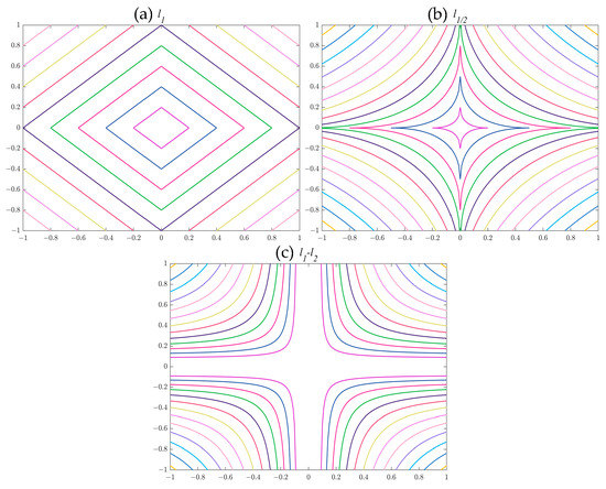
Figure 1.
level set of sparsity metric (a) L1, (b) L1/2, (c) L1–L2.
In this paper, the L1–L2 metric is introduced for sparse target image recovery, which is nonconvex yet Lipschitz continuous. The L1–L2 metric has been applied in compress sensing [35] and hyperspectral unmixing [37] to recover the sparse signal. For a matrix X, the L1–L2 metric is given by where . Compared with the Lp norm, the L1–L2 metric is parameter free and has similar convergence rates.
3.2. Total Variation Regularization
It is obvious that the IR image has poor image quality due to the abundant noise with sparse characteristics. At the same time, the building and cloud edges fluctuate greatly and will make part of the edges as the sparse components. Unfortunately, the detection of the target is also affected by these. The sparse clutters in the IR image will remain in the target image causing the false alarm.
The TV norm is successfully applied in the image denoise yield. The denoise model is formulated as follows:
where Y and X represent the observe image and clean image, respectively. is an adjustment coefficient. represents the TV norm, which can be signified as Formulation (5).
In Equation (5), m and n are the row and column numbers of the clean image and is the pixel value of an image, which is the i-th row and j-th column pixel. is the gradient of pixel at (i, j) position in the clean image.
Therefore, the TV norm is supposed to constrain the target image, since the enhanced sparsity constraint will leave little noise in the target image occupied by small pixels.
3.3. Proposed Method
As Equation (1) describes, the infrared image is regarded as a linear model, which is the sum of the target component, background component, and noise component, when the noise is approximately regarded as additive. This approach is extensively used in IR small target detection [38,39,40]. The target image can be recovered based on the sparse property of the target image and low rank property of the background image. In [21], the original image is reconstructed with the patch images, which are obtained by the sliding window on the original image. The operation transforms the original image into a patch image and can enhance the low rank of the background.
On this basis, the L1–L2 metric constraint was employed on the target image for more sparsity solution. The objective function is changed as Equation (6).
For enhancing the robustness of the algorithm to resist the structure noise, a total variation regularized constraint of target image was applied. Then, we proposed an infrared small target detection method based on nonconvex constraint based on L1–L2 norm and total variation. The final objective function is rewritten as Equation (7).
where is denoted as .
3.4. Solution of the Proposed Model
In this section, the objective function is solved with the ADMM method, and the solution is shown. The equation constraint optimization problem is converted into an unconstrained optimization problem. Thus, Equation (7) can be rewritten as the augmented Lagrangian function as Equation (8).
where denotes the inner product of two matrices, is the Frobenius norm equaling to the square root of the square sum of matrix elements, and are the Lagrangian multiplier matrixes, and is a penalty factor.
Based on the ADMM method, an alternative iteration is utilized to minimize the Lagrange function Then, the optimization problem is divided into three subproblems, and we can solve each subproblem independently. Moreover, the solution to subproblems is shown separately.
- (a)
- subproblem of B
The iteration function of B in the (k + 1) step is as follows:
The above formulation has a close-form solution obtained by a singular value thresholding shrinkage operator [41].
where U, ∑, V are acquired with the singular value decomposition (SVD) of ∑ and is the soft thresholding operator, which is written in Equation (11).
- (b)
- subproblem of T
The iteration function of T in the (k + 1) step is as follows:
However, the above formulation is a nonconvex function, due to the item being nonconvex. As mentioned in the above section, ,which can be minimized by the DCA [42]. DCA can directly linearize the objective function instead of adding constraints.
Formulation (12) is decomposed into the difference between two functions , where
For facilitating the linearization of H(T), we take an approximation of the L1–L2 metric, which is formulated as so that . The linearization of H(T) is shown as follows:
Then, the iteration solution of T can be resolved after the linearization of H(T). The solution is given as follows:
The above equitation has a closed-form solution [43], which is shown as
where is a soft-thresholding operator defined as Equation (11).
- (c)
- subproblem of F
The iteration function of F in the (k + 1) step is as follows:
The Formulation (17) is a convex function and an unconstrained optimization problem so that the minimization for (15) can be easily achieved. Then, the optimization problem is corresponding to acquiring the F, where . The derivatives of the objective function of F are shown as Equations (18) and (19):
where represents the divergence operator. To avoid the gradient of the input image being 0, the TV norm is supposed to modulate with a parameter δ. Thus, the TV norm is shown as
The Newton method is widely used to solve , The iteration solution is given as follows:
where k is the number of iterations, denotes the k-th iteration result, and d means the descending direction, which is obtained by solving with the Newton method. In addition, is the Hessian matrix at k-th iteration. However, for large scale optimization problems, the computational complexity of the inverse Hessian matrix is high. Then, the CG method is employed to solve the descending direction of the iteration equation. Thus, a solving operator is defined as follows to solve (17):
Thus, the function (22) will be solved by the Newton-CG, which is summarized in Algorithm 1.
The solving process of the nonconvex function (7) combination with the ADMM method and the solution details are summarized in Algorithm 2.
| Algorithm 1: Newton-CG algorithm for solving TV norm. |
| Input: , Output: Initialize: While not converged do Compute ; Compute (approximate Hessian matrix); Compute d; Solving with CG method; Compute ; Check the convergence conditions ; Update k k = k + 1; end |
| Algorithm 2: ADMM solver to the proposed model. |
| Input: Patch image D, Output: Target image T, Background image B Initialize: ; While not converged do %Update ; %Update ; %Update ; %Update , and ; ; ; % Judge the convergence conditions ; % Update k ; end |
3.5. The Procedure of the Proposed Method
The flow chart of the complete procedure of the proposed method is shown in Figure 2. Additionally, the particular algorithmic procedure can be summed up as follows:
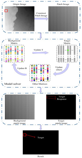
Figure 2.
The detection pipeline of the proposed model.
- Convert the original infrared image into a patch image through a sliding window with a length of len and a step of step The len and step value will be discussed in the next section;
- Parameters initialize of lambda1. The influence of the parameters on the experiments is discussed in Section 3;
- The patch image input Algorithm 1 and target patch image T solves until the iterative convergence. During iteration, the T and F iteration expressions are solved with DCA and Newton-CG methods, respectively;
- The target patch image is restored with the inverse process of step 1;
- The target detection utilizes threshold segmentation, and the segmentation is shown as Equation (23), and μ and δ denotes the mean and variance value of the separated target competent.
4. Experiments and Results
The specific experimental content will be discussed in this part. At first, the compared algorithms with their parameter settings and experimental datasets will be presented. Then, several quantitative indicators are introduced. Subsequently, the best parameters of the proposed model are selected through experiments. Finally, the datasets are tested by the proposed method and the baselines methods.
4.1. Experimental Setting
The proposed model is supposed to compare with eight SOTA methods, including local contrast measure (LCM), multiscale patch-based contrast measure (MPCM), absolute directional mean difference (ADMD) [44], infrared patch-image model (IPI), nonconvex optimization with Lp-norm constraint (NOLC), nonconvex rank approximation minimization joint L2,1 norm (NARM), and partial sum of the tensor nuclear norm (PSTNN) [45] model. The compared methods’ parameters choice was set as the authors suggested, which is given in Table 2.
Table 2.
Details of seven compared algorithms.
The proposed model is conducted on eight different scenes, four real sequences, and four single frame scenes are contained. Each frame image of the sequence datasets and the last two single frames contain only one target, while the first two single frame images contain more than one target. The scenes of the test datasets consist with various complex interference, which mainly involve the background edges with large brightness fluctuations and flickering background clutters, such as sequence 1,3 and single frame 1,4. The details of the test images are listed in Table 3.
Table 3.
Detailed descriptions of the test datasets.
4.2. Evaluation Metrics
In order to objectively illustrate the effectiveness of the proposed method, quantitative evaluation indicators are introduced. The signal-to-clutter ratio gain (SCRG) and the background suppression factor (BSF) can quantitatively describe the target enhancement and background suppression ability of the algorithms, respectively. In addition, the receiver operating characteristic (ROC) curve shows the relationship between the true positive rate (TPR) and false positive rate (FPR).
SCRG is defined as:
where SCR is an indicator to measure the significance of objectives. The numerator represents the SCR processed by the algorithm, while the denominator represents the SCR of the original image
SCR is formulated Equation (25):
where and indicate the target area’s and the neighbor region’s average pixel values. indicates the standard deviation of the neighbor area around the target position. The region size of the target and neighbor is set to 10 × 10 and 40 × 40 in the experiment.
BSF is formulated Equation (26):
where and indicates the standard deviation of the surrounding background in the input image and the standard deviation of the surrounding background in the output image. According to the formula of SCRG and BSF, the target enhancement ability and background noise suppression ability of the algorithm can be measured quantitatively. The larger SCRG and BSF, the better performance of the algorithm.
4.3. ROC Curve
ROC curve is another extensively employed evaluation in the single frame detection field, which can utilize the relationship between the FPR and TPR to illustrate the detection ability of the algorithm. TPR is supposed to demonstrate the detection proportion of the correct detection. FPR demonstrates the proportion of false alarm response which is detected as a target. As mentioned above, the algorithm has better performance when its ROC curve is closer to up and left. The TPR is formulated Equation (27):
FPR is formulated Equation (28):
4.4. Parameter Analysis
The sliding window size len, window sliding step, and lambda1 are important variables in the proposed model that have a major impact on the low rank, sparse, and iteration. For the purpose of obtaining the best results of the real dataset, it is essential to conduct sufficient experiments on the selection of key variables. Figure 3 is the ROC curve of the comparison with the parameters on the four real IR image sequences.
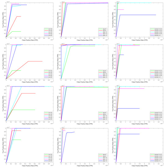
Figure 3.
Parameter setting comparison.
As depicted in Figure 3, the ROC curves obtained from the experiments from the sequences 1–4 from up to down. The ROC curves from left to right are the comparison among the len, step, and lambda1. We take the value of len as 20, 30, 40, 50, and 60, and discuss the impact on the optimization results under the condition of only changing the window size. It is seen that with the increasing of the value of len, the detection rate is increased, but when the value is 60, the detection performance begins to degrade. As the window size increases, the content in the patch is more and more abundant, and the sparse characteristic becomes more obvious. However, when the size is more than 60, the patch information is redundant, causing the sparse characteristic to degrade. This means that there is a reasonable value of len, which can make an ideal experimental result. Through the ROC curve in the first column in Figure 3, we can see that, for the fixed FPR, the TPR is the highest of the len value at 50.
For the sliding step, the variable decreases and the larger the overlapping area of the patch. Therefore, the value of the sliding step mainly affects the rank attribute of the constructed patch image. Furthermore, the smaller step will increase the dimension of the patch image and the number of calculations increases. The second column ROC curves in the Figure 3 are the comparison of the parameter of step. In addition, the value of the step is set 6, 8, 10, 12, and 14. In the experiment, the other parameters are invariant. As seen in the ROC curve, we can conclude that the value of the sliding step is 8 and can achieve a better detection performance.
As for lambda1, which is a sensitive parameter for the detection ability, the ROC curves of the comparison are shown in the third column. The value of lambda1 is set to 0.02, 0.04, 0.06, 0.08, and 0.1. The ROC curve indicates that there is an appropriate lambda1 in a reasonable range to achieve the best performance on the test data. When the value of lambda1 is 0.06, the model can detect the targets with the lowest FPR.
4.5. Comparison to SOTA
The above section discusses the vital parameters of the model, and, to confirm the robustness of the proposed model, in this section, we trial the proposed method with the SOTA methods on four real IR sequences and four single scenes. The comparison methods are listed in Table 1, including local contrast method (LCM), multiscale patch-based contrast measure (MPCM), absolute directional mean difference algorithm (ADMD), infrared patch image (IPI), nonconvex optimization with Lp-norm constraint (NOLC), nonconvex rank approximation minimization (NRAM), and partial sum of tensor nuclear norm (PSTNN). Figure 4 and Figure 5 show the performance of all algorithms on the sequence images, and Figure 6 and Figure 7 show the performance of all algorithms on the single frame images.
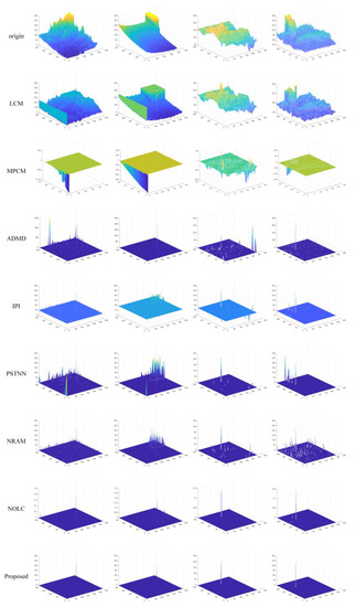
Figure 4.
3D display of sequences, original IR image, and SOTA method processing results.
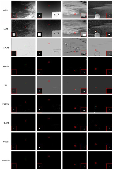
Figure 5.
Gray display of sequences, original IR image, and SOTA method processing results.
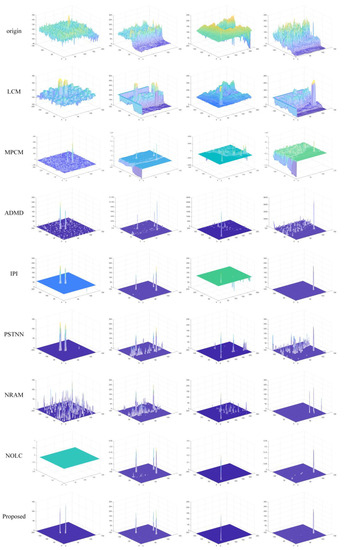
Figure 6.
3D display of single frame, original IR image, and SOTA method processing results.
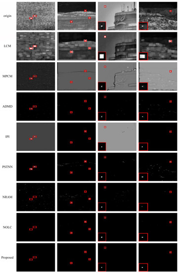
Figure 7.
Gray display of single frame, original IR image, and SOTA method processing results.
The outcomes of the proposed method and SOTA algorithms are depicted in Figure 4. The 3D displays of the results can intuitively learn about all algorithms’ detection abilities. Figure 5 displays the outcomes of comparison methods and the original IR images in gray. We make the target position in the images stand out with red rectangles and expand the target area in the images’ corners for better display.
It is obvious that the SOTA methods can eliminate the background and enhance the target to a certain extent. Nevertheless, LCM, MPCM, and ADMD have the detection performance and is relatively worse at the same FPR. Because these methods are proposed on the basis of simple assumptions, their detection ability is very poor, which is the Gaussian-like target, and the target is located at a uniform region. By comparison, the other methods are based on the low rank and sparse recovery assumption, which can obtain better results. Figure 4 and Figure 5 show that the IPI and NARM has many remaining clutters after processing. The clutters mainly obtain the edges and high bright part of the architecture. As for IPI, the simple L1 norm is employed to constrain the sparse item, resulting in a worse result, while the corner and isolate clutters are also sparse in the recovery. For NRAM, providing the surrogate, the sparse item with a weighted L1 norm for more accuracy limit the sparse item. However, it still encounters strong edge inference. The PSTNN-based IPT [46] model introduces a surrogate of the tensor rank item and unfolding of the patch-tensor to capture the low rank property. Similar to NRAM, it focuses on the low rank constraint and neglects the limit on the sparse regulation. Thus, the performances of both NRAM and PSTNN are not well suited to resist the salient clutters. The NOLC method presents the Lp norm to surrogate the L1 norm as an effective sparse constraint item and can achieve relatively better detection results compared with the methods analyzed above. However, as shown in Figure 4, there are few residual clutters in the results.
For further analysis of the abilities of all algorithms, the experiments are conducted on four single frame IR images. Figure 6 and Figure 7 show the 3D display and gray display of the results of the single frame images, respectively. In Figure 7, we made the target position in the images stand out with red rectangles and expanded the target area in the images’ corners for better display in the single target scenarios. As described in Table 2, the first and second frames contain more than one target, and the targets in the third and fourth frames are tiny and are severely interfered by the background texture. Generally speaking, the performance of optimization-based algorithms is better than the HVS-based methods at the same FPR. Then the NOLC method can achieve better background suppression by benefiting its nonconvex sparse item constraint. However, the proposed method can obtain a superior result on the test datasets in background elimination and target strengthening than NOLC. The defect of NOLC of the Lp norm is poor robustness, for it may cause a missed detection or a little higher FPR.
The ROC comparison for all methods of four real IR image sequences is advanced in Figure 8 to demonstrates the advantages of the advanced method. The horizontal axis and vertical axis are the FPR, defined as Formulation (28) and the TPR defined as Formulation (27), respectively. As seen in Figure 8, the LCM always shows the lowest TPR with the highest FPR among the comparison algorithm due to the simple local contrast feature extraction with the nine cells nest structure. The MPCM performs a little better than LCM, which can suppress the uniform background but is terrible at eliminating the complicated background. This illustrates the improved background suppression ability of MPCM compared with LCM, while LCM mainly enhanced the target with local contrast features. ADMD can achieve effective detection results on all sequences images compared with the HVS-based and background suppression-based methods. Then, the PSTNN, IPI, and NRAM have similar performance. The FPR is controlled at the low level, and the TPR is at a relatively high level. Furthermore, the NRAM keeps the lowest FPR among the three methods. The performance of NOLC is that it is the more high-performance optimization-based algorithm, which is polluted with high bright clutters causing little FPR. In general, the proposed method can obtain a better ROC on all the test sequence images, which is the lowest FPR and highest TPR among the other SOTA methods.
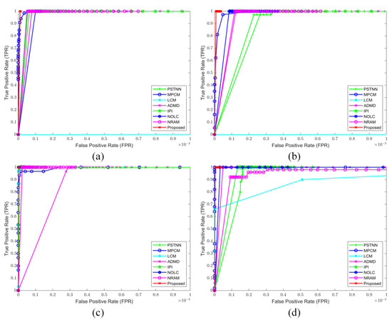
Figure 8.
(a–d) ROC curves of SOTA methods on four real sequences.
For the further quantitative evaluation of the efficiency of the advanced method, we utilized the SCRG and BSF indexes to measure the abilities of target enhancement and background suppression, respectively. The definitions of the indexes are introduced in Formulations (24) and (26). As shown in Table 4, the metrics of the proposed methods outperformed the other methods. Intuitively, the bold display shows the best two indicators. In addition, it is obvious that the optimization-based approaches show better abilities than the other methods.
Table 4.
SCRG and BSF values of the SOTA methods.
To demonstrate the real-time of the proposed method, we will analyze the computational complexity of the eight algorithms. Assuming that the size of the patch image is m×n and the original IR image size is M × N, the LCM adopts 3 × 3 template for computing so that the complexity is O(MN). Taking the multiscale into consideration and setting k sliding windows of different sizes, the final complexity is O(k3MN) where k is the number of the scales. The MPCM is the same as LCM, which calculates pixel by pixel, so the computation is also O(k3MN). For ADMD, the computation cost is mainly caused by the nested sliding window. The size of the inner window is 3 × 3, and the out window is multi-scale and is set to k. Thus, the final computation is O(8k3MN). For the IPI model, the time-consuming part is from the matrix SVD with a complexity of O(mn2). In addition, the NARM and NOLC have the same computational complexity with the IPI. The PSTNN needs to construct a tensor with the size n1 × n2 × n3, and the calculation complexity is depended on the tensor SVD and FFT operation. The FFT only conducts on the frontal slice, which the size is n1 × n2. Finally, the complexity of PSTNN is . The computational complexity of the proposed method relies on the matrix SVD and Newton-CG, and the complexity is O(nm2). It is obvious that the computational complexity of the proposed method is closely related to the size of the patch image. Furthermore, the methods based on low-rank recovery have a computational cost of O(nm2) on average. Therefore, the proposed algorithm can achieve a relatively acceptable computational complexity. The computational complexity of all methods in the experiments is summarized in Table 5.
Table 5.
Comparison of computational complexity of all methods.
5. Discussion
The background and target separation with optimization-based methods are extensively employed in the aspect of infrared small target detection. More and more researchers improve the robustness of the model with the surrogate of the nuclear norm for accurately estimating the rank of the background image or adding the additional regularization for constraining the remaining noise. The NOLC analysis is the influence of the difference between rank and sparse constraint for the IR target detection. However, the complex background edges and sparse clutters seriously interfere with the dim small target detection. In order to improve the IR small target detection model robustness under the RPCA framework, we utilized the L1–L2 norm as the sparse regularization and the total variation item to work on the target image. In Section 4, the experiments on the IR image sequences and single frames revealed that the sparse measure with L1–L2 norm could achieve an approving result in the detection tasks, though the targets were disturbed with the complex background edges and sparse clutters.
Comparing with other optimized based-methods, IPI is the beginning of the optimization-based model, which only employs the nuclear norm to estimate the rank of the background and the L1 norm as the sparse item. Therefore, the simple regularizations are inadequate to handle the complicated scenes. Making full use of the nonlocal prior information, the PSTNN extends the matrix structure to tensor structure. It mainly works at the background recovery accurately with the improved tensor nuclear norm. However, the component of the background is not strictly low rank, causing unsatisfactory recovery results facing the complex background. As shown in the experiment outcomes in Section 3, PSTNN is sensitive to the strong edges, and the tensor model ability will be limited in these scenes. As an extension of IPI, NRAM introduced the structural noise suppression regularization, which employed the L21 norm to achieve the row sparsity. However, the patch size plays an important role in structural noise elimination. If the sliding window size does not match the noise region, the effect of the regularization may not work well. Then, the NOLC improves the robustness from the perspective of the target which is different from the above mentioned one. The sparse item with the Lp norm can obtain sparser results than the L1 norm. However, the Lp norm causes missed detection and false alarms due to the selection of the value of p. The proposed method improves the robustness of the sparse item with the L1–L2 norm and adds the total variation norm to decrease the interference from strong clutters on the target perspective.
The proposed detection method utilizes the parameter free sparse item to surrogate the L0 norm, and we constrain the clutters in the target image with the total variation. Thus, the model can succeed against the challenging clutters and achieve a great detection effect.
The performance of the proposed model is illustrated by experiments. At first, we analyzed the vital parameters in the model and confirmed the optimal parameters. Then experiments were conducted on four sequences and four single frame images. Compared with the SOTA methods, the outcomes of the advanced model are the best among all the algorithms and consistent with the analysis results. The advanced model works well in both target detection accuracy and background elimination. As the results were analyzed in the experiment, the computational complexity of our algorithm did not improve. If the image size of the experiment is larger, the algorithm will take longer to run compared to the filter-based method.
6. Conclusions
In summary, the proposed approach of incorporating the L1–L2 norm and total variation regularization on the target image has significantly improved the detection accuracy of the IR small target detection model. The L1–L2 norm enhances the model’s sparsity constraint, while the TV norm strengthens its ability to reject sparse clutter interference. The resulting nonconvex model demonstrates strong performance in detecting targets and eliminating clutter, as evidenced by the ROC curve with high TPR and low FPR compared to other SOTA methods. Additionally, quantitative metrics like SCRG and BSF further validate the effectiveness of the proposed technique. Overall, this study offers a promising approach for enhancing small target detection in infrared imaging applications.
Although it is true that the proposed method has an average level of computational complexity compared to other low-rank recovery methods, it may still be more time-consuming compared to traditional filtering methods. Therefore, it is important to take into consideration the trade-off between computational efficiency and accuracy when choosing a suitable approach for the task. Additionally, further research should be conducted to improve and optimize the proposed method in order to overcome its potential limitations.
Author Contributions
Methodology, Y.S.; Validation, M.M.; Writing—original draft, Y.S.; Writing—review & editing, X.K.; Supervision, S.H.; Project administration, D.W.; Funding acquisition, C.C. and S.H. All authors have read and agreed to the published version of the manuscript.
Funding
This research was funded by National Natural Science Foundation of China (61675202, 61905240 and 62205332).
Data Availability Statement
Not applicable.
Conflicts of Interest
The authors declare no conflict of interest.
References
- Yavari, M.; Moallem, P.; Kazemi, M.; Moradi, S. Small Infrared Target Detection Using Minimum Variation Direction Interpolation. Digit. Signal Process. 2021, 117, 103174. [Google Scholar] [CrossRef]
- Guan, X.; Zhang, L.; Huang, S.; Peng, Z. Infrared Small Target Detection via Non-Convex Tensor Rank Surrogate Joint Local Contrast Energy. Remote Sens. 2020, 12, 1520. [Google Scholar] [CrossRef]
- Cai, Y. Weighted Lp—L1 Minimization Methods for Block Sparse Recovery and Rank Minimization. Anal. Appl. 2020, 19, 343–361. [Google Scholar] [CrossRef]
- Peng, C.; Liu, Y.; Kang, K.; Chen, Y.; Wu, X.; Cheng, A.; Kang, Z.; Chen, C.; Cheng, Q. Hyperspectral Image Denoising Using Nonconvex Local Low-Rank and Sparse Separation with Spatial–Spectral Total Variation Regularization. IEEE Trans. Geosci. Remote Sens. 2022, 60, 1–17. [Google Scholar] [CrossRef]
- Aragón Artacho, F.J.; Vuong, P.T. The Boosted Difference of Convex Functions Algorithm for Nonsmooth Functions. SIAM J. Optim. 2020, 30, 980–1006. [Google Scholar] [CrossRef]
- Huang, J.; Almurib, H.A.F.; Kumar, T.N.; Lombardi, F. An Inexact Newton Method For Unconstrained Total Variation-Based Image Denoising by Approximate Addition. IEEE Trans. Emerg. Top. Comput. 2022, 10, 1192–1207. [Google Scholar] [CrossRef]
- Balasingam, B.; Bar-Shalom, Y.; Willett, P.; Pattipati, K. Maximum Likelihood Detection on Images. In Proceedings of the 2017 20th International Conference on Information Fusion (Fusion), Xi’an, China, 10–13 July 2017; pp. 1–8. [Google Scholar]
- Deshpande, S.D.; Er, M.H.; Venkateswarlu, R.; Chan, P. Max-Mean and Max-Median Filters for Detection of Small Targets. In Signal and Data Processing of Small Targets; SPIE: Santa Clara, CA, USA, 1999; Volume 3809, pp. 74–83. [Google Scholar]
- Liu, R.; Wang, D.; Zhou, D.; Jia, P. Point Target Detection Based on Multiscale Morphological Filtering and an Energy Concentration Criterion. Appl. Opt. 2017, 56, 6796. [Google Scholar] [CrossRef]
- Shao, X.; Fan, H.; Lu, G.; Xu, J. An Improved Infrared Dim and Small Target Detection Algorithm Based on the Contrast Mechanism of Human Visual System. Infrared Phys. Technol. 2012, 55, 403–408. [Google Scholar] [CrossRef]
- Aghaziyarati, S.; Moradi, S.; Talebi, H. Small Infrared Target Detection Using Absolute Average Difference Weighted by Cumulative Directional Derivatives. Infrared Phys. Technol. 2019, 101, 78–87. [Google Scholar] [CrossRef]
- Bai, X.; Bi, Y. Derivative Entropy-Based Contrast Measure for Infrared Small-Target Detection. IEEE Trans. Geosci. Remote Sens. 2018, 56, 2452–2466. [Google Scholar] [CrossRef]
- Chen, C.L.P.; Li, H.; Wei, Y.; Xia, T.; Tang, Y.Y. A Local Contrast Method for Small Infrared Target Detection. IEEE Trans. Geosci. Remote Sens. 2014, 52, 574–581. [Google Scholar] [CrossRef]
- Han, J.; Ma, Y.; Zhou, B.; Fan, F.; Liang, K.; Fang, Y. A Robust Infrared Small Target Detection Algorithm Based on Human Visual System. IEEE Geosci. Remote Sens. Lett. 2014, 11, 2168–2172. [Google Scholar] [CrossRef]
- Han, J.; Liang, K.; Zhou, B.; Zhu, X.; Zhao, J.; Zhao, L. Infrared Small Target Detection Utilizing the Multiscale Relative Local Contrast Measure. IEEE Geosci. Remote Sens. Lett. 2018, 15, 612–616. [Google Scholar] [CrossRef]
- Wei, Y.; You, X.; Li, H. Multiscale Patch-Based Contrast Measure for Small Infrared Target Detection. Pattern Recognit. 2016, 58, 216–226. [Google Scholar] [CrossRef]
- Han, J.; Moradi, S.; Faramarzi, I.; Zhang, H.; Zhao, Q.; Zhang, X.; Li, N. Infrared Small Target Detection Based on the Weighted Strengthened Local Contrast Measure. IEEE Geosci. Remote Sens. Lett. 2021, 18, 1670–1674. [Google Scholar] [CrossRef]
- Shi, Y.; Wei, Y.; Yao, H.; Pan, D.; Xiao, G. High-Boost-Based Multiscale Local Contrast Measure for Infrared Small Target Detection. IEEE Geosci. Remote Sens. Lett. 2018, 15, 33–37. [Google Scholar] [CrossRef]
- Guan, X.; Peng, Z.; Huang, S.; Chen, Y. Gaussian Scale-Space Enhanced Local Contrast Measure for Small Infrared Target Detection. IEEE Geosci. Remote Sens. Lett. 2020, 17, 327–331. [Google Scholar] [CrossRef]
- Yao, S.; Chang, Y.; Qin, X. A Coarse-to-Fine Method for Infrared Small Target Detection. IEEE Geosci. Remote Sens. Lett. 2019, 16, 256–260. [Google Scholar] [CrossRef]
- Gao, C.; Meng, D.; Yang, Y.; Wang, Y.; Zhou, X.; Hauptmann, A.G. Infrared Patch-Image Model for Small Target Detection in a Single Image. IEEE Trans. Image Process. 2013, 22, 4996–5009. [Google Scholar] [CrossRef] [PubMed]
- Wang, X.; Peng, Z.; Kong, D.; Zhang, P.; He, Y. Infrared Dim Target Detection Based on Total Variation Regularization and Principal Component Pursuit. Image Vis. Comput. 2017, 63, 1–9. [Google Scholar] [CrossRef]
- Dai, Y.; Wu, Y.; Song, Y. Infrared Small Target and Background Separation via Column-Wise Weighted Robust Principal Component Analysis. Infrared Phys. Technol. 2016, 77, 421–430. [Google Scholar] [CrossRef]
- Dai, Y.; Wu, Y. Reweighted Infrared Patch-Tensor Model With Both Nonlocal and Local Priors for Single-Frame Small Target Detection. IEEE J. Sel. Top. Appl. Earth Obs. Remote Sens. 2017, 10, 3752–3767. [Google Scholar] [CrossRef]
- Zhang, Z.; Ely, G.; Aeron, S.; Hao, N.; Kilmer, M. Novel Methods for Multilinear Data Completion and De-Noising Based on Tensor-SVD. In Proceedings of the 2014 IEEE Conference on Computer Vision and Pattern Recognition, Columbus, OH, USA, 23–28 June 2014; pp. 3842–3849. [Google Scholar]
- Zhang, L.; Peng, L.; Zhang, T.; Cao, S.; Peng, Z. Infrared Small Target Detection via Non-Convex Rank Approximation Minimization Joint L2,1 Norm. Remote Sens. 2018, 10, 1821. [Google Scholar] [CrossRef]
- Zhang, T.; Wu, H.; Liu, Y.; Peng, L.; Yang, C.; Peng, Z. Infrared Small Target Detection Based on Non-Convex Optimization with Lp-Norm Constraint. Remote Sens. 2019, 11, 559. [Google Scholar] [CrossRef]
- Chartrand, R.; Staneva, V. Restricted Isometry Properties and Nonconvex Compressive Sensing. Inverse Probl. 2008, 24, 035020. [Google Scholar] [CrossRef]
- Ren, S.; He, K.; Girshick, R.; Sun, J. Faster R-CNN: Towards Real-Time Object Detection with Region Proposal Networks. IEEE Trans. Pattern Anal. Mach. Intell. 2017, 39, 1137–1149. [Google Scholar] [CrossRef]
- Fan, Z.; Bi, D.; Xiong, L.; Ma, S.; He, L.; Ding, W. Dim Infrared Image Enhancement Based on Convolutional Neural Network. Neurocomputing 2018, 272, 396–404. [Google Scholar] [CrossRef]
- Ju, M.; Luo, J.; Liu, G.; Luo, H. ISTDet: An Efficient End-to-End Neural Network for Infrared Small Target Detection. Infrared Phys. Technol. 2021, 114, 103659. [Google Scholar] [CrossRef]
- Dai, Y.; Wu, Y.; Zhou, F.; Barnard, K. Attentional Local Contrast Networks for Infrared Small Target Detection. IEEE Trans. Geosci. Remote Sens. 2021, 59, 9813–9824. [Google Scholar] [CrossRef]
- Hou, Q.; Zhang, L.; Tan, F.; Xi, Y.; Zheng, H.; Li, N. ISTDU-Net: Infrared Small-Target Detection U-Net. IEEE Geosci. Remote Sens. Lett. 2022, 19, 1–5. [Google Scholar] [CrossRef]
- Zhou, F.; Wu, Y.; Dai, Y.; Ni, K. Robust Infrared Small Target Detection via Jointly Sparse Constraint of L1/2-Metric and Dual-Graph Regularization. Remote Sens. 2020, 12, 1963. [Google Scholar] [CrossRef]
- Yin, P.; Lou, Y.; He, Q.; Xin, J. Minimization of ℓ1−2 for Compressed Sensing. SIAM J. Sci. Comput. 2015, 37, A536–A563. [Google Scholar] [CrossRef]
- Lou, Y.; Yin, P.; He, Q.; Xin, J. Computing Sparse Representation in a Highly Coherent Dictionary Based on Difference of L1 L 1 and L2 L 2. J. Sci. Comput. 2015, 64, 178–196. [Google Scholar] [CrossRef]
- Sun, L.; Ge, W.; Chen, Y.; Zhang, J.; Jeon, B. Hyperspectral Unmixing Employing l1−l2 Sparsity and Total Variation Regularization. Int. J. Remote Sens. 2018, 39, 6037–6060. [Google Scholar] [CrossRef]
- Kim, S.; Yang, Y.; Lee, J.; Park, Y. Small Target Detection Utilizing Robust Methods of the Human Visual System for IRST. J. Infrared Millim. Terahertz Waves 2009, 30, 994–1011. [Google Scholar] [CrossRef]
- Zhao, M.; Li, W.; Li, L.; Hu, J.; Ma, P.; Tao, R. Single-Frame Infrared Small-Target Detection: A Survey. IEEE Geosci. Remote Sens. Mag. 2022, 10, 87–119. [Google Scholar] [CrossRef]
- Zhang, J.; Zhang, B.; Liu, P. Infrared Small Target Detection Based on Salient Region Extraction and Gradient Vector Processing. In Proceedings of the ACM International Conference Proceeding Series; Association for Computing Machinery: New York, NY, USA, 2019; pp. 422–426. [Google Scholar]
- Cai, J.-F.; Candès, E.J.; Shen, Z. A Singular Value Thresholding Algorithm for Matrix Completion. SIAM J. Optim. 2010, 20, 1956–1982. [Google Scholar] [CrossRef]
- Zhang, F.; Yang, Z.; Wan, M.; Yang, G. Robust Principal Component Analysis Based on L1-2 Metric. In Proceedings of the 2017 4th IAPR Asian Conference on Pattern Recognition (ACPR), Nanjing, China, 26–29 November 2017; pp. 394–398. [Google Scholar]
- Yuan, M.; Lin, Y. Model Selection and Estimation in Regression with Grouped Variables. J. R. Stat. Soc. Ser. B Stat. Methodol. 2006, 68, 49–67. [Google Scholar] [CrossRef]
- Moradi, S.; Moallem, P.; Sabahi, M.F. Fast and Robust Small Infrared Target Detection Using Absolute Directional Mean Difference Algorithm. Signal Process. 2020, 177, 107727. [Google Scholar] [CrossRef]
- Zhang, L.; Peng, Z. Infrared Small Target Detection Based on Partial Sum of the Tensor Nuclear Norm. Remote Sens. 2019, 11, 382. [Google Scholar] [CrossRef]
- Zhang, X.; Ding, Q.; Luo, H.; Hui, B.; Chang, Z.; Zhang, J. Infrared Small Target Detection Based on an Image-Patch Tensor Model. Infrared Phys. Technol. 2019, 99, 55–63. [Google Scholar] [CrossRef]


Disclaimer/Publisher’s Note: The statements, opinions and data contained in all publications are solely those of the individual author(s) and contributor(s) and not of MDPI and/or the editor(s). MDPI and/or the editor(s) disclaim responsibility for any injury to people or property resulting from any ideas, methods, instructions or products referred to in the content. |
© 2023 by the authors. Licensee MDPI, Basel, Switzerland. This article is an open access article distributed under the terms and conditions of the Creative Commons Attribution (CC BY) license (https://creativecommons.org/licenses/by/4.0/).