Abstract
The estimation of forestry parameters is essential to understanding the three-dimensional structure of forests. In this respect, the potential of X-band synthetic aperture radar (SAR) has been recognized for years. Many studies have been conducted on deriving tree heights with SAR data, but few have paid attention to the effects of the canopy structure. Canopy density plays an important role since it provides information about the vertical distribution of dominant scatterers in the forest. In this study, the position of the scattering phase center (SPC) of interferometric X-band SAR data is investigated with regard to the densest vegetation layer in a deciduous and coniferous forest in Germany by applying a canopy density index from high-resolution airborne laser scanning data. Two different methods defining the densest layer are introduced and compared with the position of the TanDEM-X SPC. The results indicate that the position of the SPC often coincides with the densest layer, with mean differences ranging from −1.6 m to +0.7 m in the deciduous forest and +1.9 m in the coniferous forest. Regarding relative tree heights, the SAR signal on average penetrates up to 15% (3.4 m) of the average tree height in the coniferous forest. In the deciduous forest, the difference increases to 18% (6.2 m) during summer and 24% (8.2 m) during winter. These findings highlight the importance of considering not only tree height but also canopy density when delineating SAR-based forest heights. The vertical structure of the canopy influences the position of the SPC, and incorporating canopy density can improve the accuracy of SAR-derived forest height estimations.
1. Introduction
Forests play an important role as biotic habitats [1], areas of photosynthetic activity [2], indicators of biodiversity [3,4,5], and carbon sinks due to their potential to store large amounts of carbon over a long time [6]. Understanding the spatial variability in the three-dimensional structure of forests provides information about their biomass and habitat suitability [7]. Consequently, the estimation of forestry parameters is of great importance, particularly in terms of climate change (e.g., global carbon cycle modeling) [8,9] and for the retrieval of information regarding a forest’s biomass, its spatial distribution, and changes over time [10]. However, knowledge about these parameters may be restricted in some important ways (e.g., due to the structural and spatial complexity of the canopy), as most data are collected through field surveys within a small set of sample plots that are often selected subjectively [11,12,13]. Remote sensing with its high spatial coverage and high temporal resolution can overcome these limitations, which makes it a valuable tool for the analysis of forestry parameters [14]. In particular, data from airborne laser scanners (ALS) have been used in recent years. The ability of the laser pulses to penetrate through the canopy to a certain amount makes it a valuable tool for analyzing parameters such as tree height or stem volume [15,16,17].
Recently, ALS has demonstrated its potential for analyzing forestry parameters, offering high-resolution mapping of forests [15]. However, airborne data collection over large areas is often time-consuming and expensive compared to spaceborne techniques [8,18]. Consequently, satellite-based remote sensing plays an important role in mapping large forested areas. In recent years, many studies have been conducted using optical imagery [19,20,21,22,23]. However, since optical-based methods are often affected by cloud cover, the use of microwave satellite remote sensing, particularly synthetic aperture radar (SAR), has shown its potential for forestry applications in the last two decades. SAR remote sensing, with its active sensors, is independent of weather and light conditions [24,25] and can penetrate through a vegetation layer to a depth that is dependent on the radar wavelength [26]. This makes it a useful tool for analyzing the vertical structure of the canopy in boreal, temperate, tropical, and subtropical forests [27]. However, the penetration of the SAR signal into the canopy leads to an underestimation of tree heights. Using SAR, the tree height estimated from digital elevation models (DEM) is associated with the position of the SAR scattering phase center (SPC). Previous studies often assumed that the SPC location closely corresponds to the top tree height in forests, particularly at shorter wavelengths [28,29]. However, due to forest structure and dielectric properties, substantial penetration is frequently observed in the X- and C-bands [30,31,32]. In this study, special focus is given to the densest layer within the canopy, as it is assumed to have a substantial influence on the position of the SAR SPC. Therefore, this study aims to achieve two objectives: firstly, to analyze whether the position of the SAR SPC coincides with the densest layer of the canopy, and secondly, to investigate the influence of the layers above the densest layer, as the attenuation of the SAR signal in the upper layers may also play a significant role. By comparing the results of a deciduous and coniferous forest and employing two different definitions of canopy layer density, this study aims to provide insights into these two questions.
2. Background
In a forest, different parameters influence the properties of the backscattered SAR signal. The radar detects objects whose sizes are equal to or greater than the SAR wavelength [33]. Longer wavelengths, such as the L-band or P-band, are sensitive to the trunks of the trees, while C- and X-band microwaves scatter off the leaves, needles, and small branches within the canopy. As a result, the penetration of high-frequency systems, such as X-band systems, is expected to be limited to the top of the trees, while lower-frequency systems, such as those in the L-band, penetrate deeper into the canopy. This characteristic makes them well-suited for estimating forest biomass and other biophysical parameters [34,35,36]. However, since the SAR signal in X- and C-band data is scattered back near the top of the canopy, they are widely used for the retrieval of forest heights [25,26,31,32].
Across-track SAR interferometry is used to derive tree heights from two SAR acquisitions generated at the same time for the same area from slightly different sensor positions. As a result, since it is proportional to the surface elevation, the phase difference between the two acquisitions is used to derive the height of objects on the Earth’s surface. The phase height () can be estimated using the following equation [25]:
where unw(γ) denotes the unwrapping of the coherence coefficient , and represents the vertical wave number [37], which is related to the height of ambiguity (HoA):
In this context, the phase heights are referred to as the height of the scattering phase center of an object. However, in forests, the SPC may be located inside the canopy rather than at the top, and therefore, it may not coincide with the forest top’s height [33]. The position of the SPC results from single or multiple backscattered signals within the same volumetric resolution cell and is dependent on signal penetration [38,39]. In this work, the position of the SAR SPC is referred to as the InSAR height.
Numerous studies have investigated signal penetration in forests at different wavelengths. Most of them define the difference between the true surface elevation (e.g., as obtained by ALS data) and the location of the SPC as the penetration depth of the SAR signal [31,40,41]. However, different terms such as height bias [32], elevation bias [42], or penetration bias [39] are used synonymously. In this study, corresponds to the ALS-derived 100th percentile height (i.e., the tree top height) [43]. Consequently, the height difference between the InSAR Height and is referred to as Δh100.
In this context, it is important to note that the position of the SPC may not be solely influenced by tree height. Recent studies have not only concentrated on deriving tree heights with ALS data but have also aimed at gaining a better understanding of the vertical structure of forests. Various terms are used to describe their vertical structure, including overall relative density, normalized relative density, leaf area density, vegetation density, crown cover, canopy closure, tree cover density, and canopy density [44,45,46,47,48]. In this work, the term canopy density is used and will be described in detail in Section 4.1.2.
In the recent literature, many studies used SAR and ALS data to estimate tree height and other forestry parameters, such as aboveground biomass (AGB) and growing stock volume (GSV). Table 1 provides an overview of recent research in this field. Izzawati et al. [49] assessed the accuracy of tree height retrieval in coniferous forests using X-band interferometry and analyzed variables including crown shape, tree density, tree height, incidence angle, and slope. They found that crown shape, tree density, and tree height are the most important factors. Kugler et al. [31] investigated the potential of TanDEM-X polarimetric SAR interferometry (Pol-InSAR) for quantitative analyses of forestry parameters in two European and one tropical test site and validated the results by comparing them with ALS-derived tree heights. The authors found a strong correlation between the location of the SPC and forest top height, with correlation coefficients reaching 0.9 or higher. Moreover, seasonal differences were observed between summer and winter acquisitions in European test sites. Both Kugler et al. and Schlund et al. [31,32] analyzed the penetration depth in three test sites in Germany to apply a physical model to compensate for the penetration depth (i.e., height bias) in canopy height estimations. Substantial differences in penetration were found between leaf-on and leaf-off conditions due to the absence of leaves, leading to higher signal penetration into the canopy [32]. However, at present, no studies have linked the canopy density of different height layers to the position of the SPC. Hence, this study aims to examine the canopy structure of the forest to better understand the relationship between the SPC and canopy density and to provide answers to the aforementioned objectives, determine whether the SPC lies within the densest layers of the canopy, and explore the role of the layers above the densest layer in this context.

Table 1.
Selection of recent studies for the retrieval of forest structural parameters.
3. Study Sites and Data
3.1. Study Sites
The study sites are located in the Free State of Thuringia, central Germany. The Huss site, as part of the Hainich National Park, is located in the west of Thuringia (Figure 1), and the Roda site lies in the southeastern part of the Free State (Figure 2). The climate is temperate, with warm summers, mild winters, and mean annual precipitation of 750 mm in Hainich [53] and 600 mm in Roda [54]. Both sites have been the subject of many scientific studies to investigate forest parameters, including soil moisture, aboveground biomass (AGB), and carbon fluxes [54,55,56,57,58,59]. For this purpose, the sites were equipped with extensive measurement technology, which makes them ideal subjects for research.
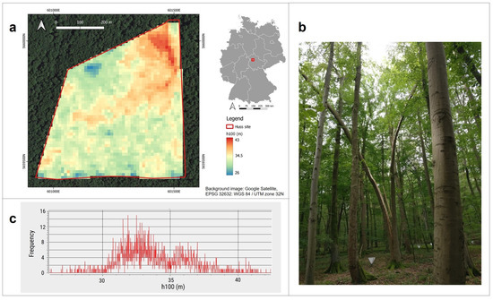
Figure 1.
Overview of the Huss supersite: (a) normalized DSM of the Huss site (boundary in red; EPSG: 32632; background: Google Satellite); (b) typical broadleaved forest in the Hainich region; (c) distribution of normalized surface heights (in m) in the Huss site in 2018. Photo: Institute of Data Science, DLR Jena.
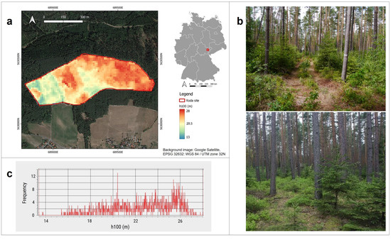
Figure 2.
Overview of the Roda site: (a) normalized DSM of the Roda site (boundary in red; EPSG: 32632; background: Google Satellite); (b) typical coniferous forest in the study site; (c) distribution of normalized surface heights (in m) in the Roda site in 2012. Photos: Department for Earth Observation, Friedrich-Schiller-University Jena.
3.1.1. Huss Supersite within the Hainich National Park
The Huss supersite lies within the Hainich National Park and covers an area of 28.2 hectares [56] (Figure 1). The Huss supersite is completely covered by dense broadleaf forest, which is primarily dominated by beech trees (Fagus sylvatica), along with other species such as ash (Fraxinus excelsior), alder (Aldus glutinosa), sycamore maple (Acer pseudoplatanus), hornbeam (Carpinus betulus), wych elm (Ulmus glabra), common and sessile oak (Quercus robur, Quercus petraea), and chequers (Sorbus torminalis) [56]. The tree heights reach up to 43 m, with an average tree height () of 34 m and a total number of more than 3500 trees. Small canopy gaps occur due to wind throws or the natural death of old trees [56]. However, the number of trees within the Huss site has not significantly changed in recent years.
3.1.2. Roda Site
The Roda site is located in the southern part of the Roda river catchment and covers an area of 23 hectares. It is predominantly populated by coniferous tree species, including Scots pines (Pinus sylvestris), Norway spruces (Picea abies), and European larches (Larix decidua) [55]. The Roda site has a of 23 m and is mainly characterized by planted and intensively managed forests [54]. Within the study site, there is a variation in tree heights from west to east (Figure 2). The western part exhibits tree heights of approximately 13 m, while the heights increase in an easterly direction, reaching their maximum at the eastern end of the study area (28 m).
3.2. Data
Two data products were utilized for the analysis: InSAR data acquired by TanDEM-X operated by the German Aerospace Center (DLR) and high-resolution ALS data provided by the Thuringian land surveying office (TLBG) for comparison [60]. Figure 3 illustrates the timeline of the data used for analysis. The data pairs were selected to have the shortest possible timespan between TanDEM-X and ALS acquisitions. For the coniferous Roda site, one pair was selected during the 2011/2012 season. In contrast, the Huss site had an additional data pair available from the 2017/2018 season. Additionally, the influence of leaf conditions at the Huss site was analyzed by considering two TanDEM-X acquisitions in 2013: one in March during leaf-off conditions and another in May during leaf-on conditions.
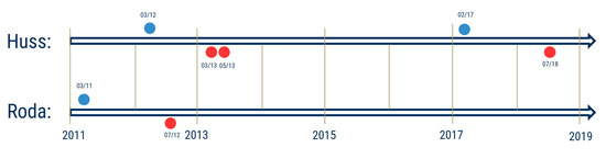
Figure 3.
Timeline of the data used in both sites, Huss and Roda (red: TanDEM-X; blue: ALS).
3.2.1. TanDEM-X InSAR Data
The TanDEM-X mission consists of two almost identical satellites, TerraSAR-X (launched in 2007) and TanDEM-X (launched in 2010). The mission provides interferometric SAR data (X-band: 9.65 GHz, 3 cm wavelength) in high spatial and temporal resolution. Its main objective is to generate a global DEM in an unprecedented spatial resolution of 12 m [61] with a relative height offset of two meters (slope < 20%) [62,63] and an absolute vertical accuracy of 10 m. The elevation values in the generated DEM represent the ellipsoidal heights relative to the WGS84 ellipsoid in the WGS84-G1150 datum [64]. One of the main advantages of the mission is the synchronous acquisition time of both satellites, which helps avoid errors caused by temporal decorrelation effects [39,65].
Four TanDEM-X InSAR scenes, all provided as analysis-ready data by DLR, were utilized in this study. To this aim, the integrated TanDEM-X processor (ITP) and the experimental TanDEM-X interferometric processor (TAXI) were used [66], where data analysis, parameter calculation, synchronization, bistatic focusing, filtering, coregistration, phase unwrapping, and geocoding is implemented in one sequence [39,67,68]. For a more detailed description of the ITP steps, refer to Fritz et al. and Zink et al. [63,67]. In this work, the data were preprocessed following the same methodology described in Martone et al. [69], with a horizontal resolution of 12 m and referenced to WGS84. Consequently, the geocoded elevation information of the DEM scenes represents the location of the mean scattering phase center, as described in Section 2 [39].
Table 2 shows the acquisition parameters of the data scenes for the two research areas. For the Huss site, two dual-pol acquisitions (HH + VV) were available in March and May 2013. The other scenes were available as single-polarized data (HH). Among all products generated through interferometric processing, only the InSAR Heights were utilized in this study, which will be described in more detail in Section 4.2.
Table 2.
TanDEM-X data takes and acquisition parameters used in this study.
3.2.2. ALS Data
To analyze the position of the SPC, the InSAR Heights were compared with discrete return airborne lidar data, which were provided by the TLBG [60]. The terrain and surface heights were downloaded as point clouds, which were already pre-classified into ground points and non-ground points. Since ALS data acquisition is expensive and time-consuming for the whole of Thuringia, the surveys only take place in a five-year cycle. Thus, only two ALS acquisitions per study area were available for the analysis, conducted in the seasons 2011/2012 and 2017/2018 (Table 3). The data underwent quality control and were horizontally referenced to ETRS89, UTM Zone 32N, and the GRS80 ellipsoid. The laser point heights (DHHN16 system) were calculated by considering the undulation between the ellipsoid and the German combined quasigeoid 2016 (GCG16), provided by the TLBG. The positional accuracy is reported to be 30 cm horizontal and 15 cm vertical [54].
Table 3.
Acquisition parameters of the ALS campaigns in Thuringia [70].
4. Methods
The methods applied in this study can be divided into two sections: the processing of ALS and TanDEM-X data and the statistical analysis to compare the InSAR Heights with the ALS data. The general workflow is illustrated in Figure 4. First, the InSAR Heights were processed using Python (version 3.8) within PyCharm Jetbrains (2021) and QGIS (version 3.18). In the second step, the ALS data were processed using LAStools (version 2021). Finally, the generated products were used to analyze Δh100 and the relationship between InSAR Height and the densest layer of the canopy. The same methodology was applied to both study sites. Results and statistical metrics (e.g., mean, median, standard deviation, etc.) were analyzed using QGIS and R (version 3.6.2) within RStudio (2019). Detailed descriptions of this procedure will be provided in the subsequent sections.
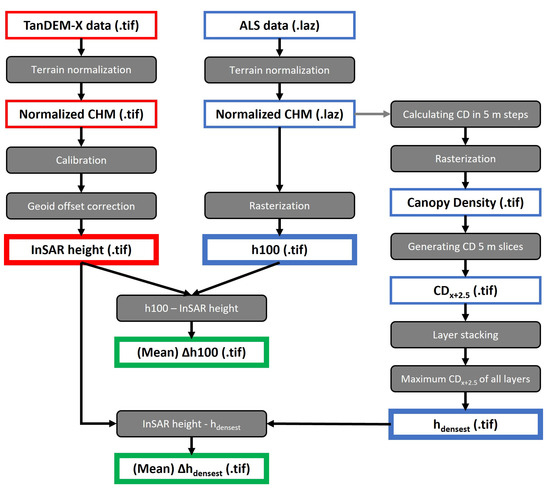
Figure 4.
Workflow applied in this study, illustrating the products resulting from the processing of TanDEM-X data (shown in red) and ALS data (shown in blue). The green rectangles show the final layers of the analysis between TanDEM-X and ALS data.
4.1. Processing of Lidar-Derived Products
4.1.1. Delineation of the Forest Top Height ()
To obtain normalized lidar-based forest heights as reference data, a point cloud provided by the TLBG was utilized for both study sites. As the point cloud is already pre-classified into ground points and non-ground points, a height-normalized point cloud was derived by subtracting the elevation of all non-ground points from the interpolated surface generated from the ground points. Subsequently, a CHM was created by gridding the point cloud into a raster model. To match the spatial resolution of the TanDEM-X data, the ALS data were processed at a resolution of 12 m. As a result, a raster layer representing the forest height was generated using the maximum height values per grid cell. All output rasters were geocoded and referenced to the WGS84/UTM zone 32 N ellipsoid (EPSG: 32632). Several studies used a similar approach [31,32,71,72,73], but generating a CHM at coarse resolutions may lead to the systematic overestimation of forest heights at some point. Therefore, some studies prefer processing the CHM at a higher resolution initially (e.g., 1 m) and then aggregating the data to a coarser resolution [26] using the average tree top height as a reference. In our study, we explored both approaches but found that the second approach resulted in lower ALS pixel heights compared to the InSAR Height. Consequently, we decided to focus solely on the first approach in the subsequent analysis.
4.1.2. Delineation of Canopy Densities and the Densest Layer of the Canopy (h)
In this study, the canopy density of a height layer is defined as the ratio of the number of points in that layer to the total number of points in all layers within the same cell and is expressed as a percentage (Figure 5). Since typically only a fraction of points falls within a given height layer, the canopy density of a specific height (CD) is calculated using the following equation:
where is the number of ALS points above that height in the grid cell, and represents the total number of ALS points in the grid cell. Consequently, the densest layer (h) in our study refers to the layer with the highest percentage of points among all layers. The reason for using relative point densities instead of absolute point densities is that the flight lines of the ALS acquisitions are characterized by different point densities, which makes comparability challenging within and between the study sites. To generate canopy density slices (i.e., height layers), the ground points from the normalized point clouds were masked out. Then, the canopy densities of the normalized vegetation point cloud were processed using LAStools and converted into a raster data format (.tif). The processing resolution was set to 12 m to ensure an adequate number of lidar points within each grid cell and to match the resolution of the TanDEM-X data. Finally, the canopy densities were divided into 5 m vertical intervals (Figure 5). This step was necessary because in LAStools, the canopy density is computed as the number of all points above a height threshold divided by the total number of points within a grid cell (as described in Equation (3)). Therefore, the conversion to 5 m intervals was carried out by subtracting the canopy density of a given height layer from the density of the layer below it, as follows:
where CD represents the canopy density of a specific height layer as a percentage, CD is the proportion of points lying above height x, and CD represents the proportion of points lying five meters above height x. This metric is also known as the overall relative density (ORD) [45].
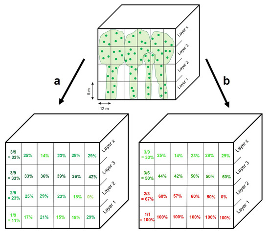
Figure 5.
Canopy density defined as (a) the number of points in a height layer x divided by the total number of points in all height layers within this grid cell (ORD) and (b) as the number of points in a height layer divided by the total number of points in all height layers below layer x (NRD). The sum of canopy densities in each grid cell is 100% for ORD and >100% for NRD. The two lowest layers in (b) were excluded from the analysis (marked in red). The resolution of the grid cell was set to 12 m, and the vertical height intervals were defined as 5 m.
Finally, the processed density layers were stacked, and the height layer with the maximum density per grid cell was extracted as h. In cases where two or more layers had the same density, the highest layer within a grid cell was chosen. Applying this method (Figure 5a), Layer 3 exhibits the highest percentages for all pixels, and thus, it would be designated as the densest layer for all six samples. Considering a 5 m vertical interval, Layer 3 represents a height between 10 m and 15 m. Consequently, the middle of this interval is defined as the center of h (12.5 m), which is utilized for comparing height differences with the InSAR Height. At this point, it can be argued that the ORD method does not account for ALS-specific effects that occur when a proportion of laser beams (i.e., all the first returns) are immediately reflected after encountering the tree tops. As a result, the highest layer of the canopy receives more energy than the layers below, reducing the total number of points reaching the lower layers. Consequently, the densest layer is more likely to be found within one of the overstory layers.
To address this issue, we developed a second method, which takes into account the reduced number of points reaching the lower layers (Figure 5b). This metric is also known as normalized relative density (NRD) [45]. In this approach, the canopy density of a height layer is calculated as the number of points in that layer divided by the total number of points below that layer within this cell. Unlike the ORD method, the NRD approach considers only the points below the layer being analyzed. As a result, higher canopy densities are observed in the understory layers, and the density is always 100% in the lowest canopy layer. The densest layer was calculated in the same way as in the ORD method. Following the NRD method, the densest layer would always be detected in the lowest layer since the canopy density is 100%. To avoid this, we excluded the two lowest layers (0–10 m) from the analysis. This is because it is unlikely for the densest layer to be found in these layers as both study sites are characterized by full-grown forest patches with tree heights greater than 10 m. However, the results of the NRD method showed a notable shift in the distribution of canopy densities, resulting in the densest layers being located 5–10 m lower compared to the ORD method. Consequently, NRD leads to higher densities in the understory and thus is likely to distort the actual point distribution between the height layers (i.e., the position of h). Due to these considerations, we decided to focus solely on the results obtained using the ORD method in our study. The height distributions of points within the point cloud are provided in Appendix A.1 for both methods and both study sites.
4.2. TanDEM-X Data Processing
To obtain terrain-normalized surface heights from TanDEM-X, the TanDEM-X-DSM was converted into a CHM by subtracting the terrain heights derived from the ALS-DTM. For this conversion, non-vegetated areas within both study sites were used as a calibration reference. Since these heights represent ellipsoidal heights relative to the WGS84 ellipsoid, while the ALS heights are based on the GCG2016 geoid, a height offset had to be considered between the two datasets. Given the fact that the height offset (i.e., geoid undulation) varies spatially, separate offsets were calculated for each study site. This offset was found to be 46.1 m for Roda and 46.2 m for Hainich [74]. Due to the relatively small size of the study areas, the offsets remained constant within each site. Consequently, the InSAR Height is given by the following equation, where U represents the individual height offset for each site:
4.3. Data Analysis between InSAR Height and Lidar-Derived Products
The data analysis focused on two main aspects regarding the relationship between TanDEM-X and ALS data, specifically the Δh100, which was used to analyze the difference between the InSAR Heights and , as well as the relationship between the canopy density, (i.e., the densest layer of the canopy) and the position of the SPC (Δh).
4.3.1. Relationship between InSAR Height and : Calculation of Δh100
As mentioned above, the height difference between InSAR Heights and ALS-derived tree top heights is referred to as Δh100 and is calculated as follows:
where represents the forest top height and is calculated as mentioned in Section 4.1.1. This is a frequently used parameter in forest applications, as well as a reference for interferometric heights [31,32,72].
For the analysis of Δh100, a complete survey was conducted in both study sites, resulting in 2045 pixels being analyzed in the Huss site and a total of 1634 pixels in Roda. In contrast to other studies [32,39,42], Δh100 was calculated by subtracting the InSAR Height from to avoid negative differences, as is normally assumed to be higher than the InSAR Height. The average difference, the median and the standard deviation between ALS and TanDEM-X heights were then calculated for the whole area. Accordingly, the mean Δh100 is calculated as follows:
To avoid negative differences, only height differences greater than 0 m were kept in the data. One can argue that analyzing only those pixels with positive differences could bias the data because the ALS beams could penetrate through small gaps in the canopy. As a result, the ALS heights may punctually be situated below the SPC. However, as both study sites are characterized by a dense canopy, negative differences are only expected due to SAR-specific geometric distortions (e.g., layover and foreshortening effects at the periphery of forest patches or clear-cut areas). Finally, to compare the different positions of the SPC in different forest types, the height difference was calculated as a percentage [49] using the ratio of the mean Δh100 and of the study site:
4.3.2. Relationship between InSAR Height and h: Calculation of Δh
For this analysis, a complete survey was conducted at both sites (Huss: 2045 pixels; Roda: 1634 pixels). In contrast to the analysis of the mean Δh100, where pixels with negative differences were eliminated, all pixels were kept in this case since the densest layer was used as reference instead of . Two analyses were conducted. First, the difference between InSAR Height and h was calculated for every densest height layer and evaluated using statistical parameters, including standard deviation, quartiles, minimum/maximum, and the analysis of variance (ANOVA). This analysis gives a good overview of the layerwise (5 m) relationship between the variables but does not allow for estimating the exact position of the SAR SPC within the canopy. Thus, in a second step, we calculated the mean difference between InSAR Height and h for all pixels within the study sites, and finally, these differences were compared for each SAR scene, polarization type, and study site according to the following equation:
where n represents the number of pixels in both of the study sites. The results were evaluated using the aforementioned statistical parameters.
5. Results
In this section, the results are presented in two subsections: the analysis of Δh100 and the relationship between InSAR Height and Δh.
5.1. Analysis of the Mean h100
Table 4 presents the mean, median, and standard deviation of Δh100 for all acquisitions at both study sites. At the Huss site, during March 2013, mean differences of more than 8 m are observed in HH polarization, and more than 7 m are observed in VV polarization. In contrast, the penetration depth remained relatively constant under leaf-on conditions, ranging from 5.6 to 6.2 m, with a minimal variation of 60 cm over the investigated time span for different polarizations. In comparison to the deciduous forest, the coniferous Roda site exhibits lower Δh100 in terms of both the mean and median (3.4 m and 3.1 m). Similar results are observed for the standard deviation, which shows considerably larger values during leaf-off conditions, particularly in HH polarization (4.3 m). The standard deviation in the coniferous forest (2.2 m) is comparable to the values obtained in the deciduous forest under leaf-on conditions (ranging from 2.3 to 2.5 m).
Table 4.
Mean and median Δh100 for all ALS/TanDEM-X data pairs in Roda and the Huss site with the corresponding standard deviations (Stdev) in meters.
To ensure comparability between the two study sites, the influence of absolute tree height variations was eliminated by converting the mean Δh100 into percentages, as described in Equation (8) in Section 4.3.1. Figure 6 presents the results for both sites. In the Huss site, with a h of 34 m, the SAR signal is scattered back at approximately 24% of the tree height in HH polarization during leaf-off conditions. However, in summer during leaf-on conditions, the signal penetrates on average only through the upper 16–18% of the canopy (Huss), indicating a clear difference compared to winter conditions. The Roda site exhibits lower differences (15% of ), meaning that the SAR signal in the coniferous forest is scattered back in slightly higher layers in relation to the average tree height in comparison to the broadleaf forest. These findings will be discussed in Section 6.
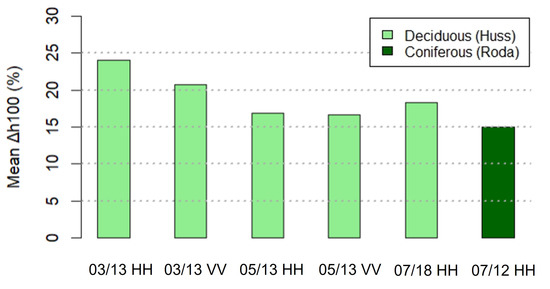
Figure 6.
Mean Δh100 (in %) relative to for all ALS/TanDEM-X data pairs at the Huss site and in Roda.
5.2. Relationship between InSAR Height and h
Figure 7 presents a boxplot comparing the InSAR Heights to h. The plot shows a significant linear relationship (p-value < 0.001) between the two variables starting from 17.5 m with small InSAR Height variances compared to the lower height layers at the Huss site (Figure 7a). However, from 27.5 m and above, the SAR signal penetrates through the center of each densest layer, resulting in height differences of +0.1 m at 27.5 m, +2.3 m at 32.5 m, and +3.3 m at 37.5 m (Figure 7b). The height layer at 27.5 m exhibits the least difference between the two variables, indicating good agreement between InSAR Height and this layer (i.e., the SPC is situated within h). Conversely, this does not apply for h lower than 27.5 m, as the SAR signal scatters back above the densest layers. In general, the differences between InSAR Height and the center of h exhibit greater variations and lower p-values at lower heights (2.5, 7.5, and 12.5), with standard deviations of up to 5 m compared to upper heights (1.7–2.4 m). The lowest densest layer shows height differences of −22.6 m, suggesting a larger influence of the upper layers on these pixels. All statistical metrics, including ANOVA, are provided in Appendix A.2 (Table A1, Table A2 and Table A3).
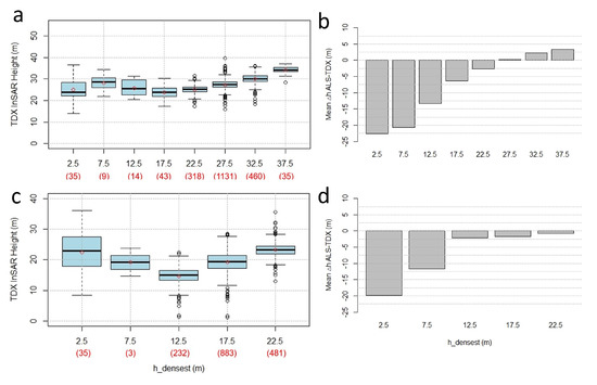
Figure 7.
InSAR Height vs. (m). Red figures: sample size per class; red dots: mean InSAR Height; black lines: median InSAR Height; the boundaries of the whiskers were set to 1.5 times the interquartile range (left) and the corresponding mean height differences per mean layer height (ALS−TanDEM-X) (right) for the Huss site in 2018 (a,b) and for Roda in 2012 (c,d).
The InSAR Heights in Roda exhibit a similar behavior to those observed at the Huss site for the lower densest layer heights (Figure 7c). In the lowest densest layer, the mean difference from the InSAR Height is −19.9 m. However, the distribution of h pixels is not evenly spread across all classes. Particularly at 7.5 m, only three pixels have their densest layer at this height, which may introduce a biased statistic and high p-values (>0.1). In contrast, starting from 12.5 m, the mean InSAR Height coincides significantly with h (Figure 7d), with mean differences ranging from −2.2 m (at 12.5 m) to −0.8 m (at 22.5 m). However, in contrast to the deciduous forest, the SAR signal does not penetrate through the center of h in any of the layers. All statistical metrics including ANOVA are provided in Appendix A.3 (Table A4, Table A5 and Table A6).
The results of the layerwise analysis can be confirmed by the statistical analysis in Table 5 and Figure 8, which examines the difference between InSAR Height and h for all pixels in the study sites (as described in Equation (9)). At the Huss site, it can be seen that the leaf-off conditions during March lead to average penetration below the center of the densest layer for both polarization types (HH: −1.6 m; VV: −0.4 m) (Figure 8). For the summer acquisitions, the mean InSAR Heights are approximately half a meter above the center of the densest layer, with only minor variations between the polarizations (ranging from 0.5 m to 0.7 m). Overall, the variability between the acquisitions (and polarizations) under leaf-on conditions is smaller compared to leaf-off conditions, with standard deviations being up to 1.7 m lower (Table 5). The same is observed in terms of interquartile ranges and minimum/maximum values of the datasets.
Table 5.
Mean and median differences between the position of the SPC and the center of h. Additionally, the standard deviation (Stdev), the lower and upper quartile (Q1, Q3), and the minimum/maximum of the distribution are shown. All values are given in meters.
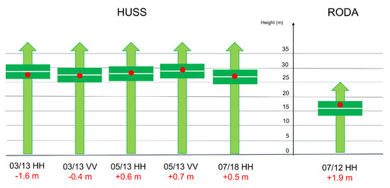
Figure 8.
Mean position of the SPC (red dots) in relation to the center of h (green rectangle, 5 m layer, center marked as a white line) for the Huss site (left) and Roda (right). The green arrows represent the stem and crown of the trees. The height variations of h are influenced by the different mean Δh100 between InSAR Height and , as well as their difference from the center of h. Red figures indicate the mean Δh.
In comparison to the deciduous forest, the mean InSAR Height at the coniferous site is considerably higher, with a difference of +1.9 m (refer to Figure 8). From a structural perspective, this observation suggests that the densest portion of coniferous tree species, such as spruces and pines, tends to be situated slightly higher in the canopy compared to deciduous trees. This finding will be further discussed in Section 6.
6. Discussion
The objective of this study was to examine the relationship between the position of the TanDEM-X SPC and the density of the canopy for different forest types, specifically deciduous and coniferous forests. In the following, the results obtained in Section 5 will be discussed in more detail.
6.1. Site Characteristics and Differences
The results revealed considerable differences between coniferous and deciduous forests, as well as variations within the individual sites. In the Huss site, the analysis resulted in generally higher mean Δh100 under leaf-off conditions (7–8 m) compared to leaf-on conditions (5–6 m). Similar findings were observed for the standard deviation, with higher values during winter (3.5–4.3 m) compared to summer (2.0–2.5 m). In deciduous forests, these differences are surprisingly high but could potentially be attributed to the coarse resolution processing of the data. However, similar results were reported by Schlund et al. [32] in Hainich, which may be primarily influenced by the absence of leaves in March [32]. Since the SAR signal in winter interacts solely with the canopy structure, the leaves in summer hinder the SAR signal to some extent from penetrating deeper into the canopy [75]. Additionally, frost potentially reduces the dielectric constant in the vegetation, leading to higher mean Δh100 [31,76] and consequently, lower positions of the SPC within the canopy. The results indicate that the mean Δh100 depends on various factors, including environmental, topographical, and acquisition parameters, and are in line with the findings of other studies [31,32,77].
The analysis comparing the two polarization types revealed generally lower mean Δh100 and standard deviations for VV polarization compared to HH. This difference could be attributed to a slightly higher ground contribution to HH polarization [31] since leaf-off conditions in March allow the SAR signal to interact more with the ground surface than under leaf-on conditions. This effect may be further increased by frozen vegetation conditions (decreased vegetation dielectric constant) as frost can occur even in March in Hainich. Consequently, both factors decrease volume attenuation, resulting in slightly higher mean Δh100 in HH polarization [31]. However, the penetration for both polarizations remained stable in summer (5–6 m), as the ground contribution in the HH polarization is minimized due to the presence of leaves and the absence of frost.
The comparison between the two sites revealed a smaller mean Δh100 in the coniferous forest (3–4 m) compared to the deciduous forest, even under leaf-on conditions (5–6 m). These results are in line with the findings of Praks et al. [50], who found a mean Δh100 of 4 m. However, the mean Δh100 in the deciduous forest was consistently lower than in the coniferous forest [50], which is inconsistent with the findings in this study. Nevertheless, when considering the mean Δh100 as a percentage relative to the average tree height, the coniferous forest exhibited a slightly smaller value (15%) compared to the deciduous forest (16–18%) (see Figure 6). Izzawati et al. [49] found that the height underestimation of TanDEM-X data is higher for cone-shaped than for ellipse-shaped crowns and strongly depends on the tree density within a forest patch. Hence, it could be argued that the higher mean Δh100 in the Huss site may be attributed to the lower tree density, as the estimated densities were approximately 350 trees/ha in Roda and 130 trees/ha in the Huss site. Additionally, only averages were used within a 12 × 12 grid cell, which could be influenced by clear-cut areas with high Δh100. However, it has to be mentioned that the number of trees per hectare was estimated only for trees taller than 5 m. Other studies accounted for undergrowth and found a tree density of approximately 330 trees/ha (stem diameter > 7 cm) in Hainich [78,79]. As the influence of undergrowth on the behavior of the SAR signal at this spatial resolution is expected to be minimal, the undergrowth was generally considered negligible in the analysis.
Another potential factor that could contribute to the observed differences is the tree height itself. Soja et al. [25] found a general increase of Δh100 with increasing tree height. Considering that the average tree height at the Huss site (34 m) is considerably higher than at the Roda site (23 m), this height difference may explain the higher penetration observed in the deciduous forest compared to the coniferous forest. As a result, it can be concluded that the InSAR Height varies across different forest types, specifically between coniferous and deciduous forests.
The layerwise analysis conducted between InSAR Height and h showed a significant linear relationship (p-values < 0.001) starting from medium tree heights in both sites. This finding supports the first objective of the study, indicating that the SPC coincides with the center of h in these layers. At the Huss site, the layer at 27.5 m showed the strongest agreement with the InSAR Height, which was found to be the layer with the most ALS points (Appendix A.1). In the lowest densest layer, considerable height differences of 20 m or more appeared in both study areas. Regarding the second objective of this study, this may indicate that the canopy density of the overstory layers is sufficiently high to hinder the SAR signal from reaching the densest layer. On the contrary, at the Huss site, the majority of these pixels are located on the forest road at the southern limit or in small clearings within the forest, and consequently, this could partly be the result of geometric distortions caused by the SAR side-looking geometry. Additionally, the uneven distribution of h samples (as seen in Figure 7), with a concentration of densest layer pixels in the upper parts of the canopy (i.e., the tree crown), could increase the influence of outliers in layers with fewer samples. In contrast to the deciduous forest, the SAR signal does not penetrate through the densest coniferous layers. This may be attributed to the different shapes of the crowns, as cone-shaped crowns are generally expected to interact differently with the SAR signal compared to ellipse-shaped crowns [49].
The analysis of mean InSAR Heights revealed that, on average, the SAR signal does not fully penetrate through h in any of the scenes (see Figure 8). However, there are noticeable differences between the polarization types. The lower mean InSAR Height in HH polarization suggests a slightly higher ground contribution, as mentioned earlier. Additionally, in HH polarization, the mean InSAR Height is more than two meters deeper in March compared to the summer acquisitions. Similar results are observed in VV polarization, but with smaller differences between March (−0.4 m) and May (+0.7 m). These findings could be attributed to the leaf-off conditions in the broadleaf forest during winter. When compared to the deciduous forest, the higher mean InSAR Height in the coniferous patch (on average 1.9 m above the center of h) suggests that the densest part of coniferous trees is located slightly higher than that of deciduous trees. Consequently, the SAR signal “gets stuck” at upper heights.
6.2. Data and Methodology
One of the challenges of comparing the InSAR Heights with was the comparatively low spatial resolution of the ALS data (12 m). This approach is used by many other studies [31,32,71,72,73], but one may argue that generating a CHM at this resolution could systematically overestimate the forest heights. On the contrary, high-resolution processing allows the laser beams to penetrate deeper into the forest, which may underestimate the forest top height [30,31,80]. In our study, we tried both approaches and found that the majority of ALS heights in the second approach were lower than the InSAR Height. Thus, we decided to consider only the first approach, which allows compensating for the underestimation of ALS-derived forest heights [31,81,82]. However, at a resolution of 12 m, the CHM loses more information compared to ALS data processed at 1 m, as multiple trees (i.e., crowns) could fall within a grid cell [83]. In terms of SAR, this mixed-pixel problem results in a combination of scattering phase centers from individual trees. As a consequence, the InSAR Height of a pixel can be influenced by different tree crowns. In this context, another limitation to consider is the relatively small size of the study areas, which may call into question the broad applicability of the results, especially in areas with heterogeneous forest stands. However, since both study sites are characterized by dense and homogeneous forest stands, they are generally assumed to provide a good representation of the characteristics of both forest types.
A further potential source of error lies in the definition and processing of canopy densities. Due to the different point densities of the ALS campaigns (as shown in Table 3), it was not possible to analyze and compare absolute canopy densities. Therefore, canopy density was defined as the ratio of the number of ALS points per height layer and grid cell to the total number of points in all layers within that grid cell (ORD). As described in Section 4.1.2, this methodology does not fully account for the attenuation of the SAR signal when penetrating through the canopy layers. Conversely, NRD ignores overstory returns to a certain amount, which would result in much higher densities in the understory [45]. According to Campbell et al. [45], it is not yet clear which of the two methods performs better or which should be preferred for estimating canopy density using discrete return lidar.
Further, it has to be mentioned that the densest layer processed according to the ORD method may not necessarily represent the actual densest part of the canopy. The ALS data were collected during winter, and consequently, the laser interacts primarily with the branches and stems of the trees. In the deciduous forest, this could lead to different densities compared to leaf-on conditions, as the presence of leaves is generally expected to lead to more ALS points within the point cloud. Additionally, the side-looking geometry of the laser beam can cause some pulses to penetrate through the canopy, hitting lower branches or the ground before producing the first return [84]. These so-called “pits” result in an underestimation of ALS points in the upper layers of the canopy. However, since the ground points are masked out in this study, the influence of these pits is expected to be minimal.
The vertical and horizontal rasterization of the forest patch allows for some potential error. The number of lidar points per square meter is specified with >4 points, and thus, the number of density values within a 1 m voxel would be quite small (e.g., 0%, 33%, 66% or 100% for 3 points within a voxel). The horizontal resolution was resampled to 12 m to match the resolution of the TanDEM-X pixels, while the vertical resolution was set to 5 m, resulting in eight height layers in Hainich and five layers in the Roda site (see Figure 7). One may argue that higher horizontal resolutions and smaller layer intervals would yield more accurate results. However, increasing the spatial resolution leads to a substantial decrease in the number of points within a voxel, leading to no-data voxels at some point. Several layer intervals between 1 m and 10 m were tested, and a 5 m layer interval was found to be the most suitable in this study. Having more lidar points per voxel would allow for smaller layer intervals, potentially improving the accuracy of the analysis. To overcome this limitation, the use of full-waveform lidar data should be considered, which can provide more detailed information about the canopy structure by utilizing statistical metrics such as the height of median energy (HOME) [85]. However, this study is based on discrete return lidar data, and therefore, the mentioned methodology using full-waveform lidar data could not be employed.
The interpretation of InSAR Heights relative to h was based on considering the mean height (e.g., 12.5 m for the layer between 10 m and 15 m) as the center of this layer. However, it should be noted that the densest part of the layer may not always be located exactly at the center. This results in a maximum potential error of 2.4 m within each densest layer. Smaller layer intervals could decrease this error but require higher point densities than those used in this study.
Another important factor to consider is the relative height accuracy of the DEM, which is specified as 2 m for flat terrain (slopes < 20°) and 4 m for mountainous regions (slopes > 20°) [62,63,86,87]. Regarding the interpretation of the data, this allows for some margin of error, as the accuracy of the InSAR Height measurements is strongly influenced by the relative height accuracy of the TanDEM-X data. Abdullahi et al. [39] took into consideration a height offset to mitigate systematic height errors by using time-staggered TanDEM-X mosaics for all acquisitions. However, as the two sites are characterized by predominantly flat terrain, it is expected that the relative height error is generally low.
In addition to tree height and canopy density, other topographic or radar-specific variables may influence the penetration behavior of X-band SAR data into the canopy. Izzawati et al. [49] investigated factors such as crown shape, incidence angle, and slope. Results from model simulations indicated that variations in viewing angle and small slopes (<30°) have minimal effects. Regarding tree density, dense canopy forests were found to have the smallest errors and the least additional errors due to slope. Thus, these effects were generally assumed as negligible in this study. Further, the incidence angle could potentially affect Δh100, but since it remained relatively constant for all acquisitions in the study sites, its influence was not further investigated (see Table 2). Additionally, longer perpendicular baselines between the acquisitions are generally expected to be more sensitive to phase noise [32]. However, the Huss site showed almost similar effective baselines, indicating comparable conditions for all acquisitions (see Table 2). In contrast, the Roda 2012 acquisition had a considerably higher baseline, which could lead to slightly more phase noise. Moreover, the oblique side-looking geometry of SAR data causes a tree height-dependent ground range offset. In this regard, Soja et al. [25] found that the difference between ascending and descending is greater for tall trees than for smaller trees.
Due to cost- and time-expensive campaigns in Thuringia, the acquisition of ALS data is conducted in a five-year cycle. In this study, the InSAR Height could not be analyzed in its phenological stages as it was carried out by Praks et al. [50]. Therefore, no conclusion can be drawn regarding seasonal differences in the SAR signal, except for spring and summer. Another factor to be considered is the time offset between the data, which ranges from 12 to 17 months. Particularly in the Huss site, the summer acquisitions may not accurately represent the true mean Δh100 since they are compared with ALS campaigns conducted in winter. These variances are generally expected to be lower in the coniferous forest. However, the long time span between the acquisitions introduces a margin of error, as small parts of the forest could have changed due to wind throws or selective logging. Since all SAR scenes were acquired after the ALS campaign, this would result in extremely high mean Δh100 in those pixels. Given that only a few trees were affected per year, the influence of this effect was generally considered low. The same applies to the Roda site. Nevertheless, the comparison between different seasons could be important at some point, as weather conditions (e.g., precipitation, soil moisture, and frost) may influence the penetration behavior of the SAR signal [31,76,88]. Moreover, forest growth could decrease the height difference between TanDEM-X and ALS data or even lead to negative Δh100, but since most trees in the study sites are mature, their growth in height was considered marginal [32].
7. Conclusions
This study focused on investigating the position of the scattering phase center of interferometric X-band SAR data in a deciduous and coniferous forest in Thuringia. The SPC was compared to high-resolution ALS data. The results revealed an unexpectedly high penetration in the X-band, with a mean Δh100 of 3.4 m in the coniferous site and approximately 6 m in the deciduous Huss site under leaf-on conditions. It was observed that the mean Δh100 was much higher under leaf-off conditions, ranging from 7.0 to 8.2 m. This is because the absence of leaves allows the SAR signal to penetrate deeper through a certain amount of the canopy. The higher difference in HH polarization may be caused by a slightly higher ground contribution compared to VV. Consequently, the SPC showed variation across different forest types. Considering relative tree heights, this corresponds to a penetration of the signal of 17–24% for broadleaved canopies and 15% for coniferous canopies. These findings suggest that the densest part of the coniferous forest is located slightly higher than in the deciduous forest, and differences in penetration may be caused by variations in crown structures.
In regard to the first hypothesis, whether the SPC is located within the densest layer of the canopy, it can be concluded that the SPC often coincides with the densest layer. The analysis of mean InSAR Heights revealed that, on average, the SAR signal does not fully penetrate through h in any of the scenes. In the deciduous site, the SPC is, on average, located between −1.6 m (leaf-off) below and +0.7 m (leaf-on) above the center of h. In the coniferous Roda site, the SAR signal is scattered back +1.9 m above the center of h, and due to its evergreen phenology, the InSAR Height is expected to show only minimal differences across all seasons. The second hypothesis, that the layers above the densest layer also influence the position of the SAR SPC, could neither be confirmed nor denied in this study. Although the SAR SPC is located considerably higher than the densest layer in the lower heights, this could also be a result of the SAR side-looking geometry and requires further investigation. However, the findings indicate that the position of the SPC is not solely determined by tree height but is also influenced by the vertical structure of the canopy. Consequently, it should also be considered an important parameter when delineating forestry parameters using SAR data.
Future work could address the factors that might have influenced the results of this analysis, including the definition of canopy density and the time difference between TanDEM-X and ALS data acquisitions. As an alternative, structure-from-motion data collected by drones could be used, as they are capable of collecting images with high spatial resolution at low operational costs [13,89,90]. Different flight patterns (e.g., nadir, oblique, and point of interest) could enhance the quality of the point cloud and facilitate the analysis of the vertical forest structure. Additionally, the analysis of mean Δh100 using drones would be possible at high temporal resolution, as their preparation is less time-consuming compared to ALS acquisitions. This would allow for the extraction of seasonal patterns regarding the position of the SPC. In this context, future work could also address the analysis of undergrowth vegetation in forested areas using different wavelengths, such as the C-band. This is particularly relevant considering that SAR data from missions such as Sentinel-1 are freely available in high temporal resolution, providing an opportunity to investigate undergrowth dynamics and their interactions with the SPC position.
Author Contributions
Conceptualization, C.D. and C.T.; methodology, J.Z., C.D. and C.T.; validation, J.Z.; formal analysis, J.Z.; investigation, J.Z.; resources, J.-L.B.-B. and P.R.; data curation, J.Z.; writing—original draft preparation, J.Z.; writing—review and editing, C.D., C.T., J.-L.B.-B., P.R. and C.S.; visualization, J.Z.; supervision, C.D. and C.T.; project administration, C.D., C.T. and C.S. All authors have read and agreed to the published version of the manuscript.
Funding
We acknowledge support by the German Research Foundation Projekt-Nr. 512648189 and the Open Access Publication Fund of the Thueringer Universitaets- und Landesbibliothek Jena.
Acknowledgments
The authors would like to thank the Thuringian land surveying office for providing ALS data and reports of the flight campaigns.
Conflicts of Interest
The authors declare no conflict of interest.
Appendix A
Appendix A.1. Comparison of Lidar Point Distribution according to the ORD and NRD Methods

Figure A1.
Distribution of points within the normalized point cloud at the Huss site in 2013 (a,b) and at the Roda site in 2012 (c,d), processed as ORD (left) and NRD (right). For the ORD method, the sum of percentages in all mean canopy layer heights (MCLH) is 100%. For NRD, the sum is higher than 100%, since the densities are calculated as proportions below the MCLH for every layer. Furthermore, the two lowest layers were excluded.

Appendix A.2. Tables Containing Statistical Parameters for the Layerwise Analysis between InSAR Height and at the Huss Site in 2018
Table A1.
Statistical parameters of the InSAR Height compared to every height of (m) at the Huss site in 2018 (HH polarization). The mean difference (Mean diff) shows the difference between the mean InSAR Height and the center of in meters. Further, the mean and median heights, the standard deviation (Stdev), the lower and upper quartile (Q1, Q3), and the minimum/maximum of the distribution are shown. All values are given in meters.
| (m) | 2.5 m | 7.5 m | 12.5 m | 17.5 m | 22.5 m | 27.5 m | 32.5 m | 37.5 m |
|---|---|---|---|---|---|---|---|---|
| Mean | 25.1 | 28.2 | 25.9 | 23.9 | 25.1 | 27.4 | 30.2 | 34.2 |
| Mean diff | −22.6 | −20.7 | −13.4 | −6.4 | −2.6 | 0.1 | 2.3 | 3.3 |
| Median | 24.0 | 28.6 | 25.6 | 23.8 | 25.3 | 27.4 | 30.1 | 34.2 |
| Stdev | 5.1 | 4.0 | 3.8 | 2.9 | 2.0 | 2.0 | 2.4 | 1.7 |
| Q1 | 22.1 | 26.0 | 23.1 | 22.0 | 24.0 | 26.2 | 28.9 | 33.4 |
| Q3 | 28.5 | 30.7 | 29.0 | 25.9 | 26.3 | 28.6 | 31.7 | 35.4 |
| Minimum | 14.1 | 22.0 | 20.4 | 17.5 | 17.3 | 15.9 | 18.3 | 28.3 |
| Maximum | 36.6 | 34.3 | 31.3 | 30.3 | 31.5 | 39.7 | 36.0 | 37.0 |
Table A2.
ANOVA table for the analysis between InSAR Height and at the Huss site in 2018. The listed parameters include the degrees of freedom (Df), the sum of squared differences (Sum Sq), the sum of squares divided by the df (Mean Sq), the F-ratio, and the p-value of the F-ratio.
Table A2.
ANOVA table for the analysis between InSAR Height and at the Huss site in 2018. The listed parameters include the degrees of freedom (Df), the sum of squared differences (Sum Sq), the sum of squares divided by the df (Mean Sq), the F-ratio, and the p-value of the F-ratio.
| Df | Sum Sq | Mean Sq | F Value | Pr (>F) | |
|---|---|---|---|---|---|
| 1 | 4745.2 | 4745.2 | 756.6 | <0.001 | |
| Residuals | 2043 | 12,812.4 | 6.3 |
Table A3.
ANOVA table for multiple pairwise comparisons between the means of all layers at the Huss site in 2018 using Tukey’s honest significant differences test. The “Difference” indicates the disparity between the mean InSAR Heights of two layers, measured in meters. Additionally, the lower and upper bounds of the 95% confidence interval are shown, along with the adjusted p-value for the multiple comparisons within each group.
| Difference | Lower (95%) | Upper (95%) | p-Value (Adj) | |
|---|---|---|---|---|
| 7.5–2.5 | 3.09 | 0.57 | 5.62 | 0.01 |
| 12.5–2.5 | 0.77 | −1.36 | 2.91 | 0.96 |
| 17.5–2.5 | −1.19 | −2.73 | 0.35 | 0.27 |
| 22.5–2.5 | 0.03 | −1.17 | 1.23 | 1.00 |
| 27.5–2.5 | 2.25 | 1.09 | 3.41 | 0.00 |
| 32.5–2.5 | 5.09 | 3.91 | 6.28 | 0.00 |
| 37.5–2.5 | 9.10 | 7.49 | 10.72 | 0.00 |
| 12.5–7.5 | −2.32 | −5.21 | 0.56 | 0.22 |
| 17.5–7.5 | −4.28 | −6.76 | −1.81 | 0.00 |
| 22.5–7.5 | −3.06 | −5.34 | −0.78 | 0.00 |
| 27.5–7.5 | −0.84 | −3.10 | 1.42 | 0.95 |
| 32.5–7.5 | 1.99 | −0.27 | 4.27 | 0.13 |
| 37.5–7.5 | 6.00 | 3.48 | 8.53 | 0.00 |
| 17.5–12.5 | −1.96 | −4.04 | 0.12 | 0.08 |
| 22.5–12.5 | −0.74 | −2.58 | 1.10 | 0.93 |
| 27.5–12.5 | 1.48 | −0.34 | 3.30 | 0.21 |
| 32.5–12.5 | 4.32 | 2.48 | 6.15 | 0.00 |
| 37.5–12.5 | 8.33 | 6.19 | 10.46 | 0.00 |
| 22.5–17.5 | 1.22 | 0.12 | 2.31 | 0.02 |
| 27.5–17.5 | 3.44 | 2.39 | 4.49 | 0.00 |
| 32.5–17.5 | 6.28 | 5.20 | 7.36 | 0.00 |
| 37.5–17.5 | 10.29 | 8.75 | 11.83 | 0.00 |
| 27.5–22.5 | 2.22 | 1.79 | 2.64 | 0.00 |
| 32.5–22.5 | 5.06 | 4.57 | 5.55 | 0.00 |
| 37.5–22.5 | 9.07 | 7.86 | 10.27 | 0.00 |
| 32.5–27.5 | 2.84 | 2.47 | 3.21 | 0.00 |
| 37.5–27.5 | 6.85 | 5.69 | 8.01 | 0.00 |
| 37.5–32.5 | 4.01 | 2.82 | 5.19 | 0.00 |
Appendix A.3. Tables Containing Statistical Parameters for the Layerwise Analysis between InSAR Height and at the Roda Site in 2012
Table A4.
Statistical parameters of the InSAR Height compared to every height of (m) at the Roda site in 2012 (HH polarization). The mean difference (Mean diff) shows the difference between the mean InSAR Height and the center of in meters. Furthermore, the mean and median heights, the standard deviation (Stdev), the lower and upper quartile (Q1, Q3), and the minimum/maximum of the distribution are shown. All values are given in meters.
| (m) | 2.5 m | 7.5 m | 12.5 m | 17.5 m | 22.5 m |
|---|---|---|---|---|---|
| Mean | 22.4 | 19.2 | 14.7 | 19.2 | 23.3 |
| Mean diff | −19.9 | −11.7 | −2.2 | −1.7 | −0.8 |
| Median | 22.9 | 19.2 | 15.0 | 19.4 | 23.2 |
| Stdev | 7.3 | 4.5 | 3.2 | 3.2 | 2.4 |
| Q1 | 18.0 | 16.9 | 13.3 | 17.2 | 22.0 |
| Q3 | 27.4 | 21.5 | 16.6 | 21.4 | 24.5 |
| Minimum | 8.5 | 14.6 | 1.4 | 1.1 | 12.9 |
| Maximum | 36.1 | 23.7 | 22.4 | 28.4 | 35.6 |
Table A5.
ANOVA table for the analysis between InSAR Height and at the Roda site in 2012. The listed parameters include the degrees of freedom (Df), the sum of squared differences (Sum Sq), the sum of squares divided by the df (Mean Sq), the F-ratio, and the p-value of the F-ratio.
Table A5.
ANOVA table for the analysis between InSAR Height and at the Roda site in 2012. The listed parameters include the degrees of freedom (Df), the sum of squared differences (Sum Sq), the sum of squares divided by the df (Mean Sq), the F-ratio, and the p-value of the F-ratio.
| Df | Sum Sq | Mean Sq | F Value | Pr(>F) | |
|---|---|---|---|---|---|
| 1 | 6563.6 | 6563.6 | 482.9 | <0.001 | |
| Residuals | 1632 | 22,182.2 | 13.6 |
Table A6.
ANOVA table for multiple pairwise comparisons between the means of all layers at the Roda site in 2012 using Tukey’s honest significant differences test. The “Difference” indicates the disparity between the mean InSAR Heights of two layers, measured in meters. Additionally, the lower and upper bounds of the 95% confidence interval are shown, along with the adjusted p-value for the multiple comparisons within each group.
| Difference | Lower (95%) | Upper (95%) | p-Value (Adj) | |
|---|---|---|---|---|
| 7.5–2.5 | −3.25 | −8.42 | 1.92 | 0.42 |
| 12.5–2.5 | −7.75 | −9.31 | −6.19 | 0.00 |
| 17.5–2.5 | −3.28 | −4.76 | −1.80 | 0.00 |
| 22.5–2.5 | 0.87 | −0.64 | 2.37 | 0.51 |
| 12.5–7.5 | −4.50 | −9.50 | 0.50 | 0.10 |
| 17.5–7.5 | −0.03 | −5.00 | 4.95 | 1.00 |
| 22.5–7.5 | 4.12 | −0.86 | 9.10 | 0.16 |
| 17.5–12.5 | 4.47 | 3.84 | 5.11 | 0.00 |
| 22.5–12.5 | 8.62 | 7.93 | 9.31 | 0.00 |
| 22.5–17.5 | 4.15 | 3.66 | 4.63 | 0.00 |
References
- Nadkarni, N.M. Diversity of species and interactions in the upper tree canopy of forest ecosystems. Am. Zool. 1994, 34, 70–78. [Google Scholar] [CrossRef]
- Carswell, F.E.; Meir, P.; Wandelli, E.V.; Bonates, L.C.M.; Kruijt, B.; Barbosa, E.M.; Nobre, A.D.; Grace, J.; Jarvis, P.G. Photosynthetic capacity in a central Amazonian rain forest. Tree Physiol. 2000, 20, 179–186. [Google Scholar] [CrossRef] [PubMed]
- Lindenmayer, D.B.; Margules, C.R.; Botkin, D.B. Indicators of Biodiversity for Ecologically Sustainable Forest Management. Conserv. Biol. 2000, 14, 941–950. [Google Scholar] [CrossRef]
- McElhinny, C.; Gibbons, P.; Brack, C.; Bauhus, J. Forest and woodland stand structural complexity: Its definition and measurement. For. Ecol. Manag. 2005, 218, 1–24. [Google Scholar] [CrossRef]
- McElhinny, C.; Gibbons, P.; Brack, C. An objective and quantitative methodology for constructing an index of stand structural complexity. For. Ecol. Manag. 2006, 235, 54–71. [Google Scholar]
- Watson, R.T.; Noble, I.R.; Bolin, B.; Ravindranath, N.H.; Verardo, D.J.; Dokken, D.J. Land Use, Land-Use Change and Forestry: A Special Report of the Intergovernmental Panel on Climate Change. 2000. Available online: https://www.cabdirect.org/cabdirect/abstract/20083294691 (accessed on 11 July 2023).
- Hensley, S.; Ahmed, R.; Chapman, B.; Hawkins, B.; Lavalle, M.; Pinto, N.; Pardini, M.; Papathanassiou, K.; Siqueria, P.; Treuhaft, R. Boreal Forest Radar Tomography at P, L and S-Bands at Berms and Delta Junction. In Proceedings of the 2020 IEEE International Geoscience & Remote Sensing Symposium, Waikoloa, HI, USA, 26 September–2 October 2020; pp. 96–99. [Google Scholar] [CrossRef]
- Karila, K.; Vastaranta, M.; Karjalainen, M.; Kaasalainen, S. Tandem-X interferometry in the prediction of forest inventory attributes in managed boreal forests. Remote Sens. Environ. 2015, 159, 259–268. [Google Scholar] [CrossRef]
- Le Toan, T.; Quegan, S.; Davidson, M.; Balzter, H.; Paillou, P.; Papathanassiou, K.; Plummer, S.; Rocca, F.; Saatchi, S.; Shugart, H.; et al. The BIOMASS mission: Mapping global forest biomass to better understand the terrestrial carbon cycle. Remote Sens. Environ. 2011, 115, 2850–2860. [Google Scholar] [CrossRef]
- Pan, Y.; Birdsey, R.A.; Fang, J.; Houghton, R.; Kauppi, P.E.; Kurz, W.A.; Phillips, O.L.; Shvidenko, A.; Lewis, S.L.; Canadell, J.G.; et al. A large and persistent carbon sink in the world’s forests. Science 2011, 333, 988–993. [Google Scholar] [CrossRef]
- Franklin, J.F.; van Pelt, R. Spatial Aspects of Structural Complexity in Old-Growth Forests. J. For. 2004, 102, 22–28. [Google Scholar] [CrossRef]
- Van Kane, R.; McGaughey, R.J.; Bakker, J.D.; Gersonde, R.F.; Lutz, J.A.; Franklin, J.F. Comparisons between field- and LiDAR-based measures of stand structural complexity. Can. J. For. Res. 2010, 40, 761–773. [Google Scholar] [CrossRef]
- Jayathunga, S.; Owari, T.; Tsuyuki, S. Evaluating the Performance of Photogrammetric Products Using Fixed-Wing UAV Imagery over a Mixed Conifer–Broadleaf Forest: Comparison with Airborne Laser Scanning. Remote Sens. 2018, 10, 187. [Google Scholar] [CrossRef]
- Boyd, D.S.; Danson, F.M. Satellite remote sensing of forest resources: Three decades of research development. Prog. Phys. Geogr. Earth Environ. 2005, 29, 1–26. [Google Scholar] [CrossRef]
- Lim, K.; Treitz, P.; Wulder, M.; St-Onge, B.; Flood, M. LiDAR remote sensing of forest structure. Prog. Phys. Geogr. Earth Environ. 2003, 27, 88–106. [Google Scholar] [CrossRef]
- Lee, A.C.; Lucas, R.M. A LiDAR-derived canopy density model for tree stem and crown mapping in Australian forests. Remote. Sens. Environ. 2007, 111, 493–518. [Google Scholar] [CrossRef]
- Latifi, H.; Heurich, M.; Hartig, F.; Müller, J.; Krzystek, P.; Jehl, H.; Dech, S. Estimating over- and understorey canopy density of temperate mixed stands by airborne LiDAR data. For. Int. J. For. Res. 2016, 89, 69–81. [Google Scholar] [CrossRef]
- Vastaranta, M. Forest Mapping and Monitoring Using Active 3D Remote Sensing. Ph.D. Thesis, University of Helsinki, Helsinki, Finland, 2012. Available online: https://helda.helsinki.fi/items/b018ccc7-6e7b-44fd-b6eb-ed4eb3ebb2aa (accessed on 11 July 2023).
- Karlson, M.; Reese, H.; Ostwald, M. Tree crown mapping in managed woodlands (parklands) of semi-arid West Africa using WorldView-2 imagery and geographic object based image analysis. Sensors 2014, 14, 22643–22669. [Google Scholar] [CrossRef]
- Ouedraogo, I.; Runge, J.; Eisenberg, J.; Barron, J.; Sawadogo-Kaboré, S. The Re-Greening of the Sahel: Natural Cyclicity or Human-Induced Change? Land 2014, 3, 1075–1090. [Google Scholar] [CrossRef]
- Brandt, M.; Hiernaux, P.; Rasmussen, K.; Mbow, C.; Kergoat, L.; Tagesson, T.; Ibrahim, Y.Z.; Wélé, A.; Tucker, C.J.; Fensholt, R. Assessing woody vegetation trends in Sahelian drylands using MODIS based seasonal metrics. Remote Sens. Environ. 2016, 183, 215–225. [Google Scholar] [CrossRef]
- Heiskanen, J.; Liu, J.; Valbuena, R.; Aynekulu, E.; Packalen, P.; Pellikka, P. Remote sensing approach for spatial planning of land management interventions in West African savannas. J. Arid. Environ. 2017, 140, 29–41. [Google Scholar] [CrossRef]
- Lambert, M.J.; Traoré, P.C.S.; Blaes, X.; Baret, P.; Defourny, P. Estimating smallholder crops production at village level from Sentinel-2 time series in Mali’s cotton belt. Remote Sens. Environ. 2018, 216, 647–657. [Google Scholar] [CrossRef]
- Tsai, Y.L.S.; Dietz, A.; Oppelt, N.; Kuenzer, C. Remote Sensing of Snow Cover Using Spaceborne SAR: A Review. Remote Sens. 2019, 11, 1456. [Google Scholar] [CrossRef]
- Soja, M.J.; Karlson, M.; Bayala, J.; Bazié, H.R.; Sanou, J.; Tankoano, B.; Eriksson, L.E.B.; Reese, H.; Ostwald, M.; Ulander, L.M.H. Mapping Tree Height in Burkina Faso Parklands with TanDEM-X. Remote Sens. 2021, 13, 2747. [Google Scholar] [CrossRef]
- Antonova, S.; Thiel, C.; Höfle, B.; Anders, K.; Helm, V.; Zwieback, S.; Marx, S.; Boike, J. Estimating tree height from TanDEM-X data at the northwestern Canadian treeline. Remote Sens. Environ. 2019, 231, 111251. [Google Scholar] [CrossRef]
- Santoro, M.; Cartus, O. Research Pathways of Forest Above-Ground Biomass Estimation Based on SAR Backscatter and Interferometric SAR Observations. Remote Sens. 2018, 10, 608. [Google Scholar] [CrossRef]
- Tanase, M.A.; Ismail, I.; Lowell, K.; Karyanto, O.; Santoro, M. Detecting and Quantifying Forest Change: The Potential of Existing C- and X-Band Radar Datasets. PLoS ONE 2015, 10, e0131079. [Google Scholar] [CrossRef]
- Schlund, M.; von Poncet, F.; Kuntz, S.; Boehm, H.D.V.; Hoekman, D.H.; Schmullius, C. TanDEM-X elevation model data for canopy height and aboveground biomass retrieval in a tropical peat swamp forest. Int. J. Remote Sens. 2016, 37, 5021–5044. [Google Scholar] [CrossRef]
- Perko, R.; Raggam, H.; Deutscher, J.; Gutjahr, K.; Schardt, M. Forest Assessment Using High Resolution SAR Data in X-Band. Remote Sens. 2011, 3, 792–815. [Google Scholar] [CrossRef]
- Kugler, F.; Schulze, D.; Hajnsek, I.; Pretzsch, H.; Papathanassiou, K.P. TanDEM-X Pol-InSAR Performance for Forest Height Estimation. IEEE Trans. Geosci. Remote Sens. 2014, 52, 6404–6422. [Google Scholar] [CrossRef]
- Schlund, M.; Baron, D.; Magdon, P.; Erasmi, S. Canopy penetration depth estimation with TanDEM-X and its compensation in temperate forests. ISPRS J. Photogramm. Remote Sens. 2019, 147, 232–241. [Google Scholar] [CrossRef]
- Ackermann, N. Growing Stock Volume Estimation in Temperate Forested Areas Using a Fusion Approach with SAR Satellites Imagery; Springer eBook Collection Earth and Environmental Science; Springer: Cham, Switzerland, 2015. [Google Scholar] [CrossRef]
- Thiel, C.; Thiel, C.; Reiche, J.; Leiterer, R.; Schmullius, C. Analysis of ASAR and PALSAR data for optimizing forest cover mapping—A GSE Forest Monitoring study. In Proceedings of the ForestSat2007, Montpellier, France, 5–7 November 2007. [Google Scholar] [CrossRef]
- Cartus, O.; Santoro, M.; Kellndorfer, J. Mapping forest aboveground biomass in the Northeastern United States with ALOS PALSAR dual-polarization L-band. Remote Sens. Environ. 2012, 124, 466–478. [Google Scholar] [CrossRef]
- Chowdhury, T.A.; Thiel, C.; Schmullius, C. Growing stock volume estimation from L-band ALOS PALSAR polarimetric coherence in Siberian forest. Remote Sens. Environ. 2014, 155, 129–144. [Google Scholar] [CrossRef]
- Chen, W.; Zheng, Q.; Xiang, H.; Chen, X.; Sakai, T. Forest canopy height estimation using polarimetric interferometric synthetic aperture radar (PolInSAR) technology based on full-polarized ALOS/PALSAR data. Remote Sens. 2021, 13, 174. [Google Scholar] [CrossRef]
- Rizzoli, P.; Martone, M.; Gonzalez, C.; Wecklich, C.; Borla Tridon, D.; Bräutigam, B.; Bachmann, M.; Schulze, D.; Fritz, T.; Huber, M.; et al. Generation and performance assessment of the global TanDEM-X digital elevation model. ISPRS J. Photogramm. Remote Sens. 2017, 132, 119–139. [Google Scholar] [CrossRef]
- Abdullahi, S.; Wessel, B.; Huber, M.; Wendleder, A.; Roth, A.; Kuenzer, C. Estimating Penetration-Related X-Band InSAR Elevation Bias: A Study over the Greenland Ice Sheet. Remote Sens. 2019, 11, 2903. [Google Scholar] [CrossRef]
- Ni, W.; Zhang, Z.; Sun, G.; Guo, Z.; He, Y. The Penetration Depth Derived from the Synthesis of ALOS/PALSAR InSAR Data and ASTER GDEM for the Mapping of Forest Biomass. Remote Sens. 2014, 6, 7303–7319. [Google Scholar] [CrossRef]
- El Hajj, M.; Baghdadi, N.; Bazzi, H.; Zribi, M. Penetration Analysis of SAR Signals in the C and L Bands for Wheat, Maize, and Grasslands. Remote Sens. 2019, 11, 31. [Google Scholar] [CrossRef]
- Dall, J. InSAR Elevation Bias Caused by Penetration Into Uniform Volumes. IEEE Trans. Geosci. Remote Sens. 2007, 45, 2319–2324. [Google Scholar] [CrossRef]
- Xu, K.; Zhao, L.; Chen, E.; Li, K.; Liu, D.; Li, T.; Li, Z.; Fan, Y. Forest Height Estimation Approach Combining P-Band and X-Band Interferometric SAR Data. Remote Sens. 2022, 14, 3070. [Google Scholar] [CrossRef]
- Lowe, T.; Moghadam, P.; Edwards, E.; Williams, J. Canopy density estimation in perennial horticulture crops using 3D spinning lidar SLAM. J. Field Robot. 2021, 38, 598–618. [Google Scholar] [CrossRef]
- Campbell, M.J.; Dennison, P.E.; Hudak, A.T.; Parham, L.M.; Butler, B.W. Quantifying understory vegetation density using small-footprint airborne lidar. Remote Sens. Environ. 2018, 215, 330–342. [Google Scholar] [CrossRef]
- Umarhadi, D.A.; Danoedoro, P.; Wicaksono, P.; Widayani, P.; Nurbandi, W.; Juniansah, A. The Comparison of Canopy Density Measurement Using UAV and Hemispherical Photography for Remote Sensing Based Mapping. In Proceedings of the 2018 4th International Conference on Science and Technology (ICST), Yogyakarta, Indonesia, 7–8 August 2018. [Google Scholar] [CrossRef]
- Umarhadi, D.A.; Danoedoro, P. Comparing canopy density measurement from UAV and hemispherical photography: An evaluation for medium resolution of remote sensing-based mapping. Int. J. Electr. Comput. Eng. 2021, 11, 356. [Google Scholar] [CrossRef]
- Chianucci, F.; Disperati, L.; Guzzi, D.; Bianchini, D.; Nardino, V.; Lastri, C.; Rindinella, A.; Corona, P. Estimation of canopy attributes in beech forests using true colour digital images from a small fixed-wing UAV. Int. J. Appl. Earth Obs. Geoinf. 2016, 47, 60–68. [Google Scholar] [CrossRef]
- Izzawati; Wallington, E.D.; Woodhouse, I.H. Forest height retrieval from commercial X-band SAR products. IEEE Trans. Geosci. Remote Sens. 2006, 44, 863–870. [Google Scholar] [CrossRef]
- Praks, J.; Demirpolat, C.; Atropov, O.; Hallikainen, M. On forest height retrieval from spaceborne X-band interferometric SAR images under variable seasonal conditions. In In Proceedings of the XXXIII Finnish URSI Convention on Radio Science and SMARAD Seminar, Espoo, Finland, 24–25 April 2013; pp. 115–118. [Google Scholar]
- Chen, Y.; Feng, Z.; Li, F.; Zhou, H.; Hakala, T.; Karjalainen, M.; Hyyppä, J. Lidar-aided analysis of boreal forest backscatter at Ku band. Int. J. Appl. Earth Obs. Geoinf. 2020, 91, 102133. [Google Scholar] [CrossRef]
- Askne, J.I.; Soja, M.J.; Ulander, L.M. Biomass estimation in a boreal forest from TanDEM-X data, lidar DTM, and the interferometric water cloud model. Remote Sens. Environ. 2017, 196, 265–278. [Google Scholar] [CrossRef]
- Mund, M.; Kutsch, W.L.; Wirth, C.; Kahl, T.; Knohl, A.; Skomarkova, M.V.; Schulze, E.D. The influence of climate and fructification on the inter-annual variability of stem growth and net primary productivity in an old-growth, mixed beech forest. Tree Physiol. 2010, 30, 689–704. [Google Scholar] [CrossRef] [PubMed]
- Adam, M.; Urbazaev, M.; Dubois, C.; Schmullius, C. Accuracy Assessment of GEDI Terrain Elevation and Canopy Height Estimates in European Temperate Forests: Influence of Environmental and Acquisition Parameters. Remote Sens. 2020, 12, 3948. [Google Scholar] [CrossRef]
- Thiel, C.; Müller, M.M.; Berger, C.; Cremer, F.; Dubois, C.; Hese, S.; Baade, J.; Klan, F.; Pathe, C. Monitoring Selective Logging in a Pine-Dominated Forest in Central Germany with Repeated Drone Flights Utilizing A Low Cost RTK Quadcopter. Drones 2020, 4, 11. [Google Scholar] [CrossRef]
- Thiel, C.; Mueller, M.M.; Epple, L.; Thau, C.; Hese, S.; Voltersen, M.; Henkel, A. UAS Imagery-Based Mapping of Coarse Wood Debris in a Natural Deciduous Forest in Central Germany (Hainich National Park). Remote Sens. 2020, 12, 3293. [Google Scholar] [CrossRef]
- Holzwarth, F.; Kahl, A.; Bauhus, J.; Wirth, C. Many ways to die-partitioning tree mortality dynamics in a near-natural mixed deciduous forest. J. Ecol. 2013, 101, 220–230. [Google Scholar] [CrossRef]
- Ratcliffe, S.; Holzwarth, F.; Nadrowski, K.; Levick, S.; Wirth, C. Tree neighbourhood matters—Tree species composition drives diversity–productivity patterns in a near-natural beech forest. For. Ecol. Manag. 2015, 335, 225–234. [Google Scholar] [CrossRef]
- Kutsch, W.L.; Persson, T.; Schrumpf, M.; Moyano, F.; Mund, M.; Andersson, S.; Ernst Detlef, S. Heterotrophic soil respiration and soil carbon dynamics in the decidous Hainich forest obtained by three approaches. Biogeochemistry 2010, 100, 167–183. [Google Scholar] [CrossRef]
- TLBG. Download Höhendaten. Available online: https://www.geoportal-th.de/de-de/Downloadbereiche/Download-Offene-Geodaten-Thüringen/Download-Höhendaten (accessed on 21 January 2022).
- Krieger, G.; Zink, M.; Bachmann, M.; Bräutigam, B.; Schulze, D.; Martone, M.; Rizzoli, P.; Steinbrecher, U.; Walter Antony, J.; de Zan, F.; et al. TanDEM-X: A radar interferometer with two formation-flying satellites. Acta Astronaut. 2013, 89, 83–98. [Google Scholar] [CrossRef]
- Steinbrecher, U.; Zink, M.; Moreira, A.; Bachmann, M.; Böer, J.; Schulze, D.; Krieger, G. TanDEM-X Mission: Overview, Status and Outlook. Int. Arch. Photogramm. Remote Sens. Spat. Inf. Sci. 2013, XL-1/W1, 327–331. [Google Scholar] [CrossRef]
- Zink, M.; Bachmann, M.; Bräutigam, B.; Fritz, T.; Hajnsek, I.; Krieger, G.; Moreira, A.; Wessel, B. TanDEM-X: Das neue globale Höhenmodell der Erde. In Handbuch der Geodäsie; Freeden, W., Rummel, R., Eds.; Springer Reference Naturwissenschaften; Springer Spektrum: Berlin/Heidelberg, Germany, 2016; pp. 1–30. [Google Scholar] [CrossRef]
- DLR. TanDEM-X Science Service System. Available online: https://tandemx-science.dlr.de/cgi-bin/wcm.pl?page=Tdm-Science-Service-System (accessed on 21 January 2022).
- Krieger, G.; Moreira, A.; Fiedler, H.; Hajnsek, I.; Werner, M.; Younis, M.; Zink, M. TanDEM-X: A Satellite Formation for High-Resolution SAR Interferometry. IEEE Trans. Geosci. Remote Sens. 2007, 45, 3317–3341. [Google Scholar] [CrossRef]
- Prats, P.; Rodriguez-Cassola, M.; Marotti, L.; Naninni, M.; Wollstadt, S.; Schulze, D.; Tous-Ramon, N.; Younis, M.; Krieger, G.; Reigber, A. Taxi: A versatile processing chain for experimental TanDEM-X product evaluation. In Proceedings of the 2010 IEEE International Geoscience and Remote Sensing Symposium, Honolulu, HI, USA, 25–30 July 2010. [Google Scholar] [CrossRef]
- Fritz, T.; Rossi, C.; Yague-Martinez, N.; Rodriguez-Gonzalez, F.; Lachaise, M.; Breit, H. Interferometric processing of TanDEM-X data. In Proceedings of the 2011 IEEE International Geoscience and Remote Sensing Symposium, Vancouver, BC, Canada, 24–29 July 2011; pp. 2428–2431. [Google Scholar] [CrossRef]
- Lachaise, M.; Fritz, T.; Bamler, R. The Dual-Baseline Phase Unwrapping Correction Framework for the TanDEM-X Mission Part 1: Theoretical Description and Algorithms. IEEE Trans. Geosci. Remote Sens. 2018, 56, 780–798. [Google Scholar] [CrossRef]
- Martone, M.; Rizzoli, P.; Wecklich, C.; González, C.; Bueso-Bello, J.L.; Valdo, P.; Schulze, D.; Zink, M.; Krieger, G.; Moreira, A. The global forest/non-forest map from TanDEM-X interferometric SAR data. Remote Sens. Environ. 2018, 205, 352–373. [Google Scholar] [CrossRef]
- TLBG. Projektberichte zu den Laserscannermessungen. Teilleistung Erfassung. PDF 2011–2020. 2021.
- Stepper, C.; Straub, C.; Pretzsch, H. Assessing height changes in a highly structured forest using regularly acquired aerial image data. For. Int. J. For. Res. 2015, 88, 304–316. [Google Scholar] [CrossRef]
- Torano Caicoya, A.; Kugler, F.; Hajnsek, I.; Papathanassiou, K.P. Large-Scale Biomass Classification in Boreal Forests With TanDEM-X Data. IEEE Trans. Geosci. Remote Sens. 2016, 54, 5935–5951. [Google Scholar] [CrossRef]
- Fatoyinbo, T.; Feliciano, E.A.; Lagomasino, D.; Lee, S.K.; Trettin, C. Estimating mangrove aboveground biomass from airborne LiDAR data: A case study from the Zambezi River delta. Environ. Res. Lett. 2018, 13, 025012. [Google Scholar] [CrossRef]
- BKG. Onlineberechnung von Quasigeoidhöhen mit dem GCG2016. Available online: http://gibs.bkg.bund.de/geoid/gscomp.php?p=g (accessed on 23 January 2022).
- Ulaby, F.T.; Wilson, E.A. Microwave attenuation properties of vegetation canopies. IEEE Trans. Geosci. Remote Sens. 1985, GE-23, 746–753. [Google Scholar] [CrossRef]
- Thiel, C.; Schmullius, C. Investigating the impact of freezing on the ALOS PALSAR InSAR phase over Siberian forests. Remote Sens. Lett. 2013, 4, 900–909. [Google Scholar] [CrossRef]
- Solberg, S.; Weydahl, D.J.; Astrup, R. Temporal Stability of X-Band Single-Pass InSAR Heights in a Spruce Forest: Effects of Acquisition Properties and Season. IEEE Trans. Geosci. Remote Sens. 2015, 53, 1607–1614. [Google Scholar] [CrossRef]
- Knohl, A.; Schulze, E.D.; Kolle, O.; Buchmann, N. Large carbon uptake by an unmanaged 250-year-old deciduous forest in Central Germany. Agric. For. Meteorol. 2003, 118, 151–167. [Google Scholar] [CrossRef]
- Anthoni, P.M.; Knohl, A.; Rebmann, C.; Freibauer, A.; Mund, M.; Ziegler, W.; Kolle, O.; Schulze, E.D. Forest and agricultural land-use-dependent CO2 exchange in Thuringia, Germany. Glob. Chang. Biol. 2004, 10, 2005–2019. [Google Scholar] [CrossRef]
- Nilson, M. Prediction of forest variables using LIDAR measurement with different footprint size and measurement densities. Proceedings of ScandLaser, Umea, Sweden, 2–4 September 2003; pp. 124–132. [Google Scholar]
- Aulinger, T.; Mette, T.; Papathanassion, K.; Hajnsek, I.; Heurich, M.; Krzystek, P. Validation of Heights from Interferometric SAR and LIDAR over the Temperate Forest Site“Nationalpark Bayerischer Wald”. In Proceedings of the POLinSAR 2005 Workshop, Frascati, Italy, 17–21 January 2005; Volume 586, p. 11. Available online: https://adsabs.harvard.edu/full/2005ESASP.586...11A (accessed on 11 July 2023).
- Hajnsek, I.; Kugler, F.; Lee, S.K.; Papathanassiou, K.P. Tropical-forest-parameter estimation by means of Pol-InSAR: The INDREX-II campaign. IEEE Trans. Geosci. Remote Sens. 2009, 47, 481–493. [Google Scholar] [CrossRef]
- Hsieh, P.F.; Lee, L.C.; Chen, N.Y. Effect of spatial resolution on classification errors of pure and mixed pixels in remote sensing. IEEE Trans. Geosci. Remote Sens. 2001, 39, 2657–2663. [Google Scholar] [CrossRef]
- Khosravipour, A.; Skidmore, A.; Isenburg, M.; Wang, T.; Hussin, Y. Generating pit-free canopy height models from airborne lidar. Photogramm. Eng. Remote Sens. 2014, 80, 863–872. [Google Scholar] [CrossRef]
- Drake, J.B.; Dubayah, R.O.; Knox, R.G.; Clark, D.B.; Blair, J.B. Sensitivity of large-footprint lidar to canopy structure and biomass in a neotropical rainforest. Remote Sens. Environ. 2002, 81, 378–392. [Google Scholar] [CrossRef]
- Zink, M.; Bachmann, M.; Brautigam, B.; Fritz, T.; Hajnsek, I.; Moreira, A.; Wessel, B.; Krieger, G. TanDEM-X: The New Global DEM Takes Shape. IEEE Geosci. Remote Sens. Mag. 2014, 2, 8–23. [Google Scholar] [CrossRef]
- Hong, S.H.; Wdowinski, S.; Amelung, F.; Kim, H.C.; Won, J.S.; Kim, S.W. Using TanDEM-X Pursuit Monostatic Observations with a Large Perpendicular Baseline to Extract Glacial Topography. Remote Sens. 2018, 10, 1851. [Google Scholar] [CrossRef]
- Gorrab, A.; Zribi, M.; Baghdadi, N.; Lili-Chabaane, Z.; Mougenot, B. Multi-frequency analysis of soil moisture vertical heterogeneity effect on radar backscatter. In In Proceedings of the 2014 1st International Conference on Advanced Technologies for Signal and Image Processing (ATSIP), Sousse, Tunisia, 17–19 March 2014; pp. 379–384. [Google Scholar] [CrossRef]
- Lim, Y.S.; La, P.H.; Park, J.S.; Lee, M.H.; Pyeon, M.W.; Kim, J.I. Calculation of Tree Height and Canopy Crown from Drone Images Using Segmentation. J. Korean Soc. Surv. Geod. Photogramm. Cartogr. 2015, 33, 605–614. [Google Scholar] [CrossRef]
- Jin, C.; Oh, C.y.; Shin, S.; Wilfred Njungwi, N.; Choi, C. A Comparative Study to Evaluate Accuracy on Canopy Height and Density Using UAV, ALS, and Fieldwork. Forests 2020, 11, 241. [Google Scholar] [CrossRef]


Disclaimer/Publisher’s Note: The statements, opinions and data contained in all publications are solely those of the individual author(s) and contributor(s) and not of MDPI and/or the editor(s). MDPI and/or the editor(s) disclaim responsibility for any injury to people or property resulting from any ideas, methods, instructions or products referred to in the content. |
© 2023 by the authors. Licensee MDPI, Basel, Switzerland. This article is an open access article distributed under the terms and conditions of the Creative Commons Attribution (CC BY) license (https://creativecommons.org/licenses/by/4.0/).