Article

Towards a Guideline for UAV-Based Data Acquisition for Geomorphic Applications

1
Department of Earth Sciences, Indian Institute of Technology Kanpur, Kanpur 208016, India
2
Institute of Geosciences, University of Potsdam, 14476 Potsdam, Germany
*
Author to whom correspondence should be addressed.
Remote Sens. 2023, 15(14), 3692; https://doi.org/10.3390/rs15143692
Submission received: 20 May 2023 / Revised: 14 July 2023 / Accepted: 16 July 2023 / Published: 24 July 2023

Abstract

:
Recent years have seen a rapid rise in the generation of high-resolution topographic data using custom-built or commercial-grade Unmanned Aerial Vehicles (UAVs). Though several studies have demonstrated the application potential of UAV data, significant knowledge gaps still exist in terms of proper documentation of protocols for data acquisition, post-flight data processing, error assessments, and their mitigation. This work documents and provides guidelines for UAV data acquisition and processing from several years of field experience in diverse geomorphic settings across India, including undulating topography (~17 km2), alluvial plains (~142 km2), lowland-river basin (~66 km2), and a highly urbanized area (~5 km2). A total of 37,065 images with 16 and 20 Megapixels and 604 ground control points (GCPs) were captured with multiple UAV systems and processed to generate point clouds for a total area of ~230 km2. The Root Mean Square Error (RMSE) for each GCP for all sites ranged from 6.41 cm to 36.54 cm. This manuscript documents a comprehensive guideline for (a) pre-field flight planning and data acquisition, (b) generation and removal of noise and errors of the point cloud, and (c) generation of orthoimages and digital elevation models. We demonstrate that a well-distributed and not necessarily uniformly distributed GCP placement can significantly reduce doming error and other artifacts. We emphasize the need for using separate camera calibration parameters for each flight and demonstrate that errors in camera calibration can significantly impact the accuracy of the point cloud. Accordingly, we have evaluated the stability of lens calibration parameters between consumer-grade and professional cameras and have suggested measures for noise removal in the point cloud data. We have also identified and analyzed various errors during point cloud processing. These include systematic doming errors, errors during orthoimage and DEM generation, and errors related to water bodies. Mitigation strategies for various errors have also been discussed. Finally, we have assessed the accuracy of our point cloud data for different geomorphic settings. We concluded that the accuracy is influenced by Ground Sampling Distance (GSD), topographic features, and the placement, density, and distribution of GCPs. This guideline presented in this paper can be extremely beneficial to both experienced long-term users and newcomers for planning the UAV-based topographic survey and processing the data acquired.

1. Introduction

The advent and adaptation of Unmanned Aerial Vehicles (UAVs) for photogrammetric analysis have enhanced opportunities in remote sensing in recent years. With the availability of custom-made and consumer-grade UAV systems, high-resolution images are easier to acquire. The affordability of consumer-grade UAVs has attracted researchers from various scientific applications, such as mapping architectural heritages [1,2], vegetation monitoring [3,4,5], species identification and habitat assessment [6,7], monitoring greenhouse gas emission [8], aquaculture monitoring [9,10,11], coastal area monitoring [12,13,14], water resources monitoring [15,16], monitoring mining hazards [17,18], landslide and natural hazard monitoring [19,20], soil moisture estimation [21], flood risk monitoring [22,23], geomorphic change detection [24,25], and morphometric analysis [26,27]. However, high-quality data acquisition and processing protocols for geomorphic research and development are still poorly documented.
Most importantly, several of these studies do not contain the information necessary to reproduce data acquisition and processing. Specifically, the protocols for flight planning and ground control points (GCPs) collection, choice of appropriate tools (hardware and software) and parameters, filtering steps for the generation of reliable point clouds using Structure from Motion (SfM) techniques [25,28,29], their classification for enhancing terrain characterization, and point cloud error assessments are seldom documented. Also, there is rarely any documentation or guideline on data quality and the quantification and comparison of inherited errors of consumer-grade equipment with that of professional grade, for scientific study [30]. As a result, researchers rely heavily on self-learning processes, which are challenging and time-consuming, especially for those with lesser UAV piloting and data-processing experience.
For UAV surveys, flight preparation and planning are the most crucial steps for successful data acquisition. Unplanned or poorly planned UAV flights may result in long field campaigns, instrument damage, or, worse, loss of life. Longer field campaigns will eventually increase project costs and multiply the overall risk factors [31]. Therefore, careful pre-flight planning is necessary for surveying large areas where landscape diversity might provide several challenges, e.g., a sudden change in topography or tree line or proximity to restricted airspace. The presence of a river may lead to stronger winds and may jeopardize the flight. Contemporary works seldom highlight these operational limitations [3,32,33,34].
Numerous studies have been conducted to reduce the distortion of output resulting from the natural variations in lens systems, using controlled environments with consistent topography, predefined points, and small study areas [35,36,37,38,39]. The use of (1) converging images from multiple angles, (2) calibrated cameras, and (3) Ground Control Points (GCPs) have been shown to significantly reduce the doming or dishing effects associated with unsuccessful camera calibration. However, there is a lack of research documenting the deformation and positional errors in variable topographical outdoor-based UAV acquisitions with limited controls. Also, there is a lack of information about the deformation, such as warping artifacts, which may result from human error and lead to undesired effects in the gridded Digital Elevation Model (DEM).
Positional errors are often quantified by the Root Means Square Error (RMSE), which calculates the absolute distances between GCPs and those from the model (DEM or orthophoto). Generally, an RMSE of 2.5–4.0 cm [29,40] is reported when the flight plan ensures a significant overlap (70–95%) between images supplemented with evenly distributed GCPs. While building a DEM of a glacier system [41] in the Alps, vertical and horizontal accuracies of 0.10–0.25 m and 0.03–0.09 m, respectively, were obtained. Similar studies also achieved high accuracy for small areas (<2 km2) [42,43,44]. The horizontal and vertical accuracy can be improved using a UAV equipped with a navigation grade Global Navigational Satellite System (GNSS) and differential processing [20].
For small sites (<2 km2), several works by multiple researchers have used a high density of GCPs exceeding 200 GCPs/km2 to attain high accuracy. However, acquiring such dense GCP network is unrealistic where the survey area spans several square kilometers, and the study is constrained by time, resources, and infrastructure access. Researchers can also choose low-relief GCP sites that are devoid of shrubs or urban structures and generally have more consistent topography. In contrast, large area surveying extends over multitudes of structures and topography, for example, buildings, roadways, water bodies, barren lands, forests, and mountains which increases the challenges in obtaining quality GCPs with high accuracy. Thus, there should be a balance between the number of placed GCPs due to time constrain and desired accuracy.
The present work aims to address these knowledge gaps and provide guidelines for (a) pre-flight preparations, (b) post-flight data processing and evaluation, including point cloud classification and analysis, and (c) identification of the challenges, errors, and mitigation strategies associated with acquiring high-resolution datasets. The errors and mitigation strategies are discussed, and they have been applied and tested over diverse terrains. Point clouds were generated using the commercially available Agisoft Metashape Professional (AMP) Version 1.8.3 build 14298 (64-Bit, Educational License), which is the primary photogrammetry software used in this work unless stated otherwise. Point cloud classification and raster generation were mostly carried out with an educational version of Lastools from Rapidlasso [45]. Point cloud and rasters were handled and viewed with open-source software such as QGIS, pdal [46], displaz [47], and Cloud Compare (CC) [48].

2. Study Sites, Instruments, and Datasets

We have selected four sites from India representing diverse geomorphic settings: (1) undulating terrain with low hills and valleys (Mandsaur, Madhya Pradesh); (2) mixed land use terrain (Mayurbhanj, Odisha); (3) a lowland river basin (Sakri river basin, Kawardha, Chhattisgarh); and (4) an urbanized area (Anpara thermal power plant, Uttar Pradesh) (Figure 1). Table 1 lists the details of the UAV flights for each site. Additional details, UAV images, and DEMs of the study sites are provided in Supplementary Section S1.
Each site is associated with unique challenges and terrain characteristics. Mandsaur site (1) represents terrain traversed by multiple small but mostly dry rivers. It is almost barren except for isolated bushes and short trees on the banks of the dry river. Mayurbhanj site (2) represents the largest of all sites and consists of a mixture of forested land, agricultural lands, hills, large infrastructures, villages and towns. Kawardha site (3) covers a small river basin (Sakri). The area has multiple land uses, including forests, hills, and a large urban area. The Anpara thermal power plant site (4) is a highly urbanized area and is characterized by multiple water bodies and manmade structures, such as power plants, housing colonies, dumping yards, and high-voltage power lines.
During multiple field campaigns spanning almost five years (2015–2019), aerial and GNSS data were captured simultaneously for each study area. Aerial images were captured by either a fixed-wing Trimble—UX5 with Sony Alpha NEX-5T camera or a Quadcopter DJI Phantom 4 pro with its proprietary camera (model FC6310) while the Trimble R10-V10 was used to collect GNSS data. The NEX-5T camera is a fixed-lens 16 MP camera with a focal length of 25 mm. The Phantom 4 Pro camera is also a fixed lens 20 MP camera with a focal length of 8.8 mm. There were two identical sets of NEX-5T cameras—RGB (Red-Green-Blue) and RGNIR (Red-Green-Near InfraRed). The RGNIR camera is equipped with the same fixed lens as the RGB camera, except that the blue band is replaced with a NIR band. In every project, the RGB camera was used except at Mandsaur (1). While flying in Mandsaur (1), the RGB camera malfunctioned after three flights and was unable to capture additional images. It was replaced with the RGNIR camera for the rest of the mission. Since the return intensity from healthy vegetation in the NIR is greater than that from the vegetation-free ground, dense vegetation cover results in pronounced blue colors, an effect observed in Mandsaur (1).

3. Approach and Methodology

The UAV data acquisition and processing typically involved five steps: (1) pre-flight planning, including UAV selection and GCP collection strategy; (2) UAV flights and DGPS survey; (3) post-flight data processing involving advanced photogrammetry software for generating 3D point cloud data; (4) error assessment and mitigation; and (5) generation of DEM and ortho-photos and their accuracy assessment (Figure 2).

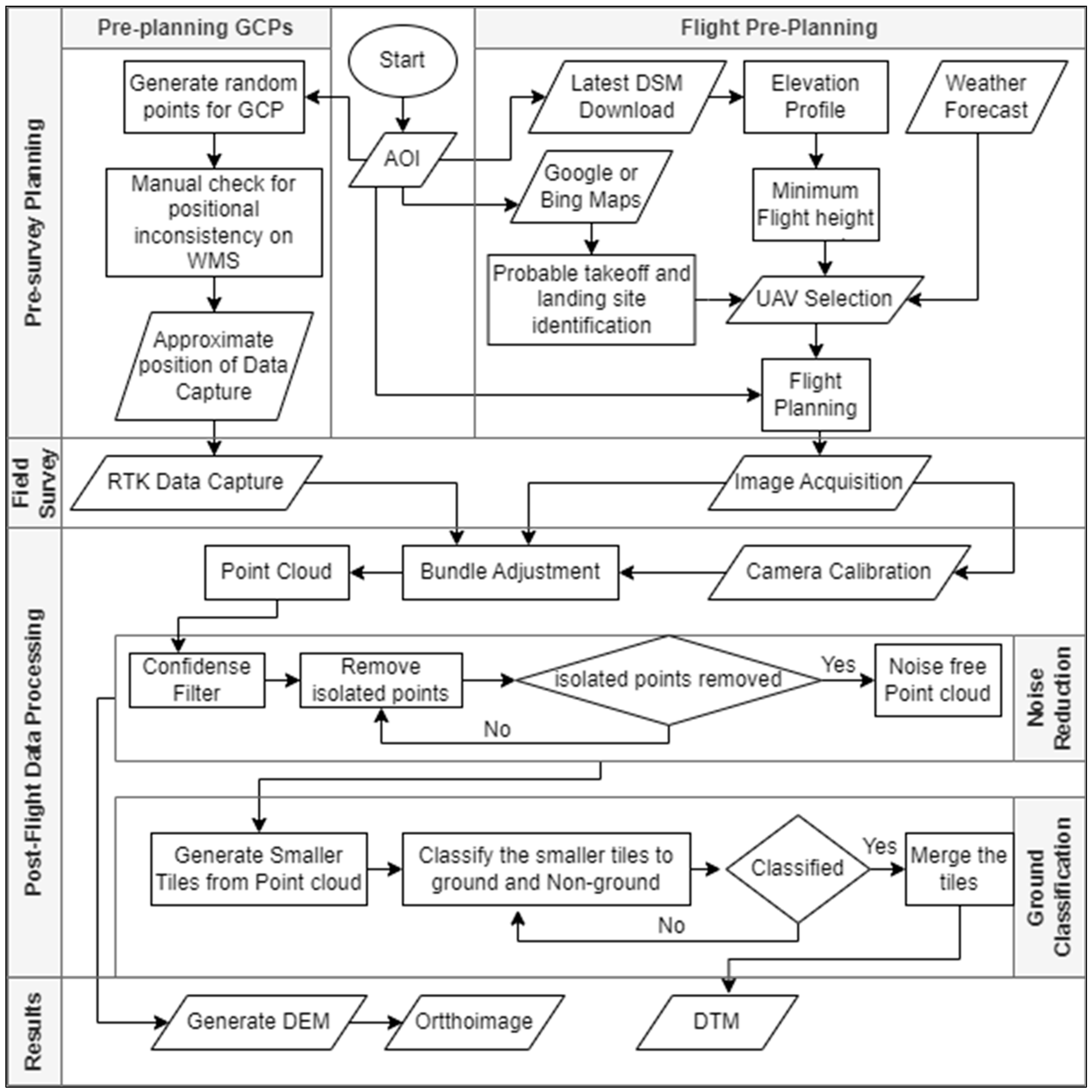
3.1. Pre-Flight Planning (Including UAV Selection and GCP Collection Strategy)

The mapping area was identified on Google Earth and exported to a GIS system (QGIS). Elevation profiles were generated using the SRTM DEM to extract the minimum and maximum heights of the study area, which guided us in determining the minimum flight height. A proper Ground Sampling Distance (GSD) was chosen to balance the limitations of aviation rules (400 feet or approximately 120 m as per Federation Aviation Administration, USA) and project requirements. The GSD varied for each project depending on the flight height. A buffer of 3 flight lines was added to the mapping area, expanding the boundary and thereby preventing lower image counts at the edges.
The terrain was examined using Google, Bing WMS, or aerial photos for preparing pre-flight contingency plans, which included identification of (a) launching and landing sites, (b) emergency landing sites, (c) potential air turbulence areas, (d) restricted airspace zones, (e) crowded regions, and (f) potential bird nesting areas. The choice of UAV depends upon the extent of the survey, landing conditions and the takeoff zone. For a large area survey with ample landing and takeoff space, a fixed-wing UAV is preferred. Vertical takeoff and landing-capable UAVs are ideal for constrained regions, for example, areas covered or surrounded by large trees. The GCPs were pre-planned by generating random points in QGIS, preferably at least one per square kilometer, to ensure uniformity in distribution (Figure 3). It is desirable that a slightly larger number of random points are generated for GCPs, as several locations may not be accessible in the field. The GCP targets had a dimension of 1 m × 1 m and were created by pasting two A4 size black papers over a white A3 sheet, placed diagonally.

3.2. DGPS Survey and UAV Flights

For topographic surveys, the GCPs were collected before the UAV flights in two ways: (a) target markers (targets made from contrasting colors—preferably black and white), and (b) corners of permanent structures that could be easily visible and distinguishable in the aerial images. In the field, a Trimble R10 GNSS system was used to collect the GCPs in RTK mode. The GNSS base station was established on relatively higher ground for wide coverage, and the baseline distance was always kept below 10 km. When the distance exceeded 10 km, we daisy-chained a new base using the old base. The base was observed in static mode for a minimum of thirty minutes before locking the base coordinates. We first positioned the GNSS rover over the GCP and waited for a minimum of 25 s. We took 45 measurements in one-second intervals and averaged them. Structures that could be seen and distinguished from the air were chosen for locations where GCP targets were not used. Random points were generated within the survey area using the GIS platform to guarantee an even distribution of GCPs. A buffer of 500–1000 m (dependent on project) was chosen for the GCP targets since these points were randomly produced and may be affected by access restrictions.
A schedule was developed after subdividing the study region according to the flight plan. Prior to the UAV flights, the GCP targets were laid out and measured. An example is shown in Figure 3, where random points with uniform distribution were generated over Mayurbhanj (2). However, several anthropogenic disturbances can lead to the loss of GCP markers, requiring the reacquisition of data. Further, information about neighboring communication towers and high-tension overhead wires is not readily available, and therefore, the potential launch and landing sites should be carefully examined. In India, high-tension lines operate at voltages between 11 and 33 kilovolts, which could interfere with the UAV’s ability to communicate with its controller. This problem was experienced at Anpara (4), where multiple manual flights were made between the high-tension lines to reduce disruption of communication. Further, it is advisable to carry out UAV flights between 9:30 and 14:30 local time, when the shadows are short, and the sun has a near-nadir inclination angle. While capturing images over water bodies, it is preferable to avoid the noon sunlight (11:00–13:00 h) as that may result in unwanted reflection artifacts.

3.3. Post-Flight Image Processing

The first major task of post-flight data processing is image alignment, which involves a few mandatory and optional steps that are common to most photogrammetry software. These processes comprise camera (lens) calibration, image bundle adjustment, GCP positioning, and dense-point cloud generation (Figure 2). We present a brief description of each step here, and further details are provided in Section 4 and Supplementary Section S2.

3.3.1. Camera (Lens) Calibration

Different cameras were used during the image capture period. Mandsaur (1) and Mayurbhanj (2) sites were captured using the Sony NEX-5T. Kawardha (3) and Anpara (4) sites were captured with an RGB proprietary camera from DJI (FC6310) attached to the UAV (DJI Phantom 4 Pro). Every image captured by a camera documents its extrinsic parameters consisting of orientation (rotational and translational) data and a few intrinsic data (e.g., focal length, number of pixels). The images from NEX-5T do not embed extrinsic parameters into the image metadata and generate a separate text file. In contrast, the FC6310 embeds information into the metadata.
Lens distortions are the primary errors affecting the images. All objects projected onto the image plane through the camera lens suffer a deviation from the central axis. The radial/optical distortion is symmetric due to the lens’s inherent structure. It may be exacerbated by material inconsistency such as microbubbles, surface or sensor defects, and uncertainties, for example, imprecise sensor size. Since such physical inhomogeneities are always present in field conditions, image points deviate from their original positions. Several manufacturing defects can be mitigated through a simple correction model describing a lens distortion. These distortions have been extensively studied by the photogrammetry community and are often solved by applying different distortion models, which relate the pixel coordinates of undistorted and distorted images [49,50].
Photogrammetry software first generates key points for each image. In Metashape, a ‘key point’ is a scale-invariant feature and represents a distinctive gradient in an image. When a key point is found and linked to multiple images, it is referred to as a ‘tie point’. These tie points can be used to solve camera calibration parameters and camera position, such as optical center, pixel skewness, and lens distortions [51]. Several data acquisition campaigns calibrate their camera before takeoff to provide better inversion constraints when solving for the camera model [52].
The original model was developed for correcting lens distortion in close-range photogrammetry [53]. It assumes that radial distortion can be described by a polynomial equation. The coefficients are determined with images from a calibration board and measuring their deviation from undistorted positions. In our work, we have used AMP for camera calibration, which relies on a modified version of Brown’s distortion model [54]. It generates a matrix for intrinsic parameters and combines it with the extrinsic parameters, generating 3D points from 2D image coordinates.
x = X/Z
y = Y/Z
x’ = x (1+ k1r2 + k2r4 + k3r6) + p2(r2 + 2x2) + 2p1xy
y’ = y (1 + k1r2 + k2r4 + k3r6) + p1(r2 + 2y2) + 2p2xy
u = cx + x’fx + y’skew
v = cy + y’fy
r2 = x2 + y2
Wherein, X, Y, and Z are the point coordinates in the local camera coordinate system. x-y and x’-y’ represent undistorted and distorted projected coordinates on the image frame. k1, k2, and k3 are the radial distortion coefficients, and p1 and p2—tangential distortion coefficients. r is the radial distance from the optical center. Further, u and v are the projected point coordinates in the image coordinate system in pixels, and fx and fy are the focal lengths in the respective axis. cx and cy are the principal point coordinates. Here, skew is the skew coefficients between the x- and y-axis.
For field acquisitions with limited numbers of ground control points and usually horizontal geometry, it is generally suggested to solve for three radial lens distortion parameters (k1, k2, k3), two tangential lens distortion parameters (p1, p2), and the center coordinates. Higher-order correction parameters (k4, b1, and b2) are often not supported in outdoor settings but may be used for indoor camera calibration.
Other than the optical error, the camera system can also be subjected to external factors like the vibration/shaking of the UAV [55]. A high shutter speed and gimbal can drastically reduce this impact during image acquisition [56]. It is useful to calculate and store camera distortion parameters on a regular basis to identify lens changes. They will differ between geographic locations if temperature and pressure change [57]. A comparison of the lens calibration system is provided in Section 4.1.
Multiple scenarios can be envisioned to analyze the impact of intrinsic camera calibration parameters on the resulting point cloud. We present three scenarios which were applied on a cluster of 3328 images (three UAV flights—1029, 1146, and 1153 images per flight) captured by the RGB Sony NEX-5T over Mandsaur (1) area and 12 GCPs uniformly spread over the total area.
  • Case 1: The camera’s intrinsic parameters were generated from 40 images of a calibration board (On-screen board in AMP) from different angles. We used a flat-screen IPS (In-Plane Switching) display with 178 degrees of viewing angle for calibration. The derived model was used as a starting point and was optimized during the bundle adjustment stage. No GCPs were used. This camera model was used for processing all images.
  • Case 2: The camera intrinsic parameters were determined separately for each flight during bundle adjustment within AMP. We did not use any pre-calibrated values as starting points. We first grouped all images as per flight and then performed bundle adjustments for each group of images (group 1: 1029 images, group 2: 1146 images, and group 3: 1153 images) without GCPs, producing individual lens models for each flight. The image groups were merged (remember—lens models were not merged), and all 12 GCPs were placed, followed by another bundle adjustment.
  • Case 3: All images were processed together (a single group containing 3328 images), 12 GCPs were placed, and bundle adjustment generated a single intrinsic model for the camera that applies to all flights. The image bundle was realigned, and the intrinsic parameters were optimized.
To evaluate differences, point clouds and orthophotos were compared. The 3328 photos from the three flights were recorded on the same day to reduce inconsistency. Each flight took between 35 and 40 min to complete. As each flight originated from the same home point, the time between corresponding landing and takeoff times were all within ten minutes, and the total flight time was two hours and thirty minutes. This area receives ample sunlight, and the maximum temperature exceeds 42 °C. So, there were notable changes in ambient brightness and temperature during the flight period. We collected a total of 18 GCPs but used only 12 GCPs within the perimeter of the three flights to generate the point cloud.
Only the parameters k1, k2, k3, cx, cy, p1, and p2 were optimized. For each scenario, the intrinsic properties of the lens were calculated, and point clouds were generated. The point cloud for case scenarios 1, 2, and 3 are named P1, P2, and P3, respectively. All models were compared for scale, distortion, and positional errors. The point clouds were first registered with each other using the Iterative Closest Point (ICP) method, and then point-to-point distances were calculated in CloudCompare. We observed multiple sources of errors in the resultant point cloud and have proposed mitigation strategies in the results section.

3.3.2. Image Bundle Adjustment and Filtering

After the initial image alignment and optimization step, the key points or scale-invariant features can be used to generate a low-density point cloud that will help to place GCPs. This product is sometimes referred to as a sparse point cloud. We used the standard AMP settings of 40,000 tie points and 4000 key points per image. Blurred and oblique images were removed from the processing prior to key point detection.
An optional step to improve positioning accuracy and camera calibration is to filter the sparse point cloud by (re-)projection attributes. This is implemented through a series of filters in ‘Gradual selection’ in AMP. Existing literature describes assumptions, methodological background, and applied thresholds [30], but we emphasize that parameters may need to be adjusted locally. We have applied several filtering steps to remove points with low projection accuracies, for example, points that were only detected in a limited number of image pairs or where the image (2D) to 3D coordinates were uncertain. The goal of these iterative filtering steps is to produce a sparse point cloud with fewer but more precise points that better describe camera locations and lens calibration parameters.

3.3.3. GCP Positioning and Camera Optimization

The process was completed in two steps. In the first step, the GCPs were positioned on the UAV images coinciding with the central pixel of the targets or the corner of the structures. We manually clicked more than five images containing the target. Markers with less than five images were ignored, removed from the calculations, and used as validation markers for assessing accuracy. Most of the GCPs with less than five images are due to the removal of markers by anthropogenic or natural disturbances. A few GCPs were also rejected as they were shadowed by buildings or not identifiable from the images. Only images with a clear view of the marker were used. After precisely clicking a few images, the automatic marker detection in AMP can help in identifying markers on new images, speeding up the manual steps. The image alignment process was iterated along with the placement of each GCP, ensuring the inclusion of GCPs as tie points while re-positioning the images. To decrease processing load and increase GCP placement speed, we only optimized camera (image) positions by forcing the camera calibration to remain constant.
In the final step, once all GCPs were positioned, we reset and recalculated the alignment. This step generated optimized camera parameters and positions (intrinsic and extrinsic) using GCPs as stationary tie points. This camera configuration was used for bundle adjustment and dense-point cloud generation, described in the next section.

3.3.4. Dense Point Cloud Generation, Noise Removal/Reduction, and Ground Classification

The dense point cloud is the most significant output generated from the photogrammetric steps. The dense point clouds were developed after downscaling images by a factor of 4 (2 times by each side) to optimize storage space, signal-to-noise ratio (SNR), and processing time (Supplementary Section S2).
We further filtered the dense point cloud by the number of image pairs used to generate the depth maps. This is called “confidence” in AMP and refers to the number of pairs (e.g., 4 overlapping photos will have (n − 1)! = 6 pairs). Points with less than three pairs were removed. This point cloud was further filtered through an outlier detection method, such as a statistical outlier filter implemented in either Lastools (lasnoise) from Rapidlasso [45] or pdal [58]. The point cloud was tiled into smaller files (preferably 200–100 m tile sizes) to prevent memory issues with a buffer overlap of 5–10 m to allow parallel processing (lasnoise).
After noise removal, ground detection was performed using morphological filters, either using Lastools (lasground) [59] or pdal (Simple Morphological Filter) [60]. The classified point cloud tiles were merged to form a noise-free point cloud (i.e., containing all classes and only removing noise class while merging the tiles) and a point cloud containing only ground-classified points. The ground-classified point cloud was used for Digital Terrain Model (DTM) generation, whereas the noise-free point cloud containing all classes was used for DSM generation.

3.3.5. Generation of DEM/DTM/Orthoimage and Accuracy Assessment

A TIN-based interpolation routine implemented in Blast2dem from Lastools was used for interpolating a grid from the point cloud. TIN-based interpolation allows for filling gaps through linear interpolation. A comprehensive analysis of the differences in raster images generated from two different methodologies is presented in Section 4.2.2.
AMP was used to generate the orthoimage in the respective GSD of the study areas. One can use either a mesh or a gridded surface model (DSM) to generate the orthomosaic, and we have used the DSM. We imported the noise-free point cloud and a DSM into AMP for generating the orthoimages. The DTM and the ground point cloud should not be used to generate the orthoimages as they may contain interpolated areas and result in gaps or artifacts.
Accuracy assessment is an integral part of data generation. In UAV-based data processing for DEM generation, accuracy can be internal or external. Internal accuracy indicates the geometrical deformation or relative or scaling error of the point cloud. The external accuracy is generally measured as the deviation of the DEM or orthomosaic from the GNSS values (GCP coordinates and altitudes). The deviation, which may be expressed as RMSE (Root Mean Square Error), was computed in the x, y, and z direction (RMSEx, RMSEy, RMSEz, respectively) and the total RMSE (RMSEr) using the following equations:
R M S E x = X U A V X G C P 2 n
R M S E y = X U A V X G C P 2 n
R M S E z = Z U A V Z G C P 2 n
R M S E r = R M S E x 2 + R M S E y 2 + R M S E z 2
In this work, the GCPs are used to primarily check the RMSEz, because we expect the vertical RMSE to be the largest.

4. Results and Discussion

This section presents the mitigation results of different errors generated during data processing which will lead to high distortion of the topographic model with unrealistic values. We also demonstrate the efficacy of the methodology developed in this work.

4.1. Stability of Lens Calibration

Lens calibration parameters of multiple missions were extracted and compiled for each camera system to understand their variability (Table 2. As both cameras are different systems, we normalized the variation by their mean:
Variation (in %) = (Standard Deviation)/Mean
A total of 28 flights were used to generate the NEX-5T camera calibration over the Mayurbhanj (2) area. For FC6310, 18 flights were used over the Kawardha (3) site. The radial variation (k2 = 79.73%) and tangential (p1 = 49.77%) distortions in FC6310, a consumer-grade camera, are higher than that of NEX-5T. Both cameras, particularly the NEX-5T, showed high stability in their lens calibration. This can be attributed to a more stable lens setup. The survey-grade camera has a telecentric lens (compound lens) system, wherein multiple lenses are used on the same axis so that light rays are incident perpendicularly on the sensor [56], greatly reducing perspective distortion. This lens system also optimizes other factors influencing lens calibration, such as focus time and level (leading to sharper edges of the subjects) [61], reduced noise level (as more light enters the camera and sensor gain can be kept low), uniform illumination of the subjects (due to reduced vignette effects), and a consistent tilt angle along the sensor plane (near parallel rays of light). Contrarily, the FC6310 has a focus range between 1 m and infinity (endocentric camera), which mimics the eye and experiences perspective distortions. In this type of distortion, light rays obliquely incident on the sensor and produce additional errors.

4.2. Point Cloud Error Identification and Mitigation

Here, we document some of the causes, effects, and mitigation procedures for several errors we encountered during the topographic surveys, which are a combination of mechanical faults, low-image quality, algorithmic limitations, or human-induced errors.

4.2.1. Systematic Doming Errors

In UAV photogrammetry, minimizing systematic doming errors takes the highest precedence and is expressed as central doming or dishing of an area [36,62]. As we used a fixed-wing UAV, the use of convergent images was not feasible, but the adaptive camera modeling and other mitigation methods decreased the error to a large extent, as discussed below.
(a)
Effect of GCP on systematic doming
Using uniformly spaced GCPs is an effective and popular step to minimize the doming error, but obtaining uniformly spaced GCPs is seldom possible in field conditions. Here, we use data acquired from one of our sites, Mandsaur (1), for the assessment and mitigation of the doming error using well-distributed GCPs (n = 40). To measure the extent of this error at Mandsaur (1), the distance between point clouds was computed and compared rather than using individual GCPs. The maximum displacement between the nearest neighbor points between the point clouds using the Hausdorff distance [63] was calculated in Cloud Compare using two sets of pre-generated point clouds: (a) point cloud with n = 40 GCP called P-A and (b) Point Cloud without GCP called P-B.
Figure 4a shows that P-B suffers a noticeable bowl-shaped systematic error, concaving upward compared to P-A. The concavity starts at the center with errors less than 2.16 m, increasing gradually outward up to 17 m at the edges, approximately 2.1 km from the center of the bowl. The mean elevation difference is 5.47 m, with a standard deviation of 2.76 m. The elevation difference is plotted in a histogram, and a distinctive unimodal pattern emerges (Figure 4b).
The GCPs aid during bundle adjustment by providing additional constraints during matrix inversion. Our findings are in line with previous studies suggesting that the GCPs significantly improve the accuracy of the DEMs [36,38,50,64,65]. Also, while surveying large areas, which may include a variety of terrains such as water bodies, barren lands, forests, mountains, and other variables such as buildings and roadways, it is not possible to choose uniform topography, which increases the difficulty of achieving improved accuracy. The general advice is to space GCPs at least at the four corners and in the center of the area to survey. In this example at Mandsaur (1), we used 40 GCPs over an area of 14 km2, resulting in a density of 3 GCPs per km2. Our results are in contrast to earlier trials [66] with a higher GCP density of 20 GCPs per hectare (i.e., 540 GCPs per km2), and we suggest that well-distributed but not necessarily uniformly spaced GCPs can prevent the doming by serving as anchorage points for the model.
(b)
Effect of camera calibration on systematic doming
Three sets of camera optimization parameters were generated from the three cases described in Section 3.3.1 (Table 3). We aim to segregate the errors caused by deformation, rotation, scaling, and lateral and horizontal shifts under these conditions and compare them. There are two ways of comparison—using either rasters or point clouds. Rasters are more suitable for visualization, while point clouds retain 3D and structural information.
To compare, we first directly converted the point clouds from Case 1, Case 2, and Case 3 to DEMs and calculated the RMSEz using 18 GCPs (Table 4). It shows that Case 2 has the lowest errors. Thus, for all other comparisons, the point cloud and DEMs generated from Case 2 are considered as the reference.
We subsampled the point clouds with densities of 37.83 to 38.14 points/m2 to a lower density of 1 point/m2 (Table 5) to reduce computational load. Subsampling was done using the point closest to the centroid of the 1 m grid. The total number of points decreased to 3.73 × 10⁶. We refer to the corresponding subsampled point clouds for Case 1, Case 2, and Case 3 as P1, P2, and P3, respectively. We then aligned the point clouds P1 and P3 to the reference point cloud P2 using ICP.
Both point clouds (P1 and P3) did not experience scaling errors, and the boundaries matched (Table 6). The final registration RMSE was calculated over 3.73 × 10⁶ points and resulted in 0.15 m and 1.39 m for P1 and P3, respectively. No rotational change was observed between P1 and P2, but a rotation of 0.2 degrees was calculated between P1 and P3. Also, the center of P3 observed an RMS shift of 9.21 m.
The registered point clouds were used to generate the DEMs (D1, D2, and D3 for the corresponding P1, P2, and P3) and the orthomosaic. Figure 5a shows the distribution of the z-distances between the DEMs D1 to D2 (dZd1d2) derived from the aligned point clouds P1 and P2. These show minimum deviation from the base DEM (D2). However, we observed a significant difference between D3 and D2 (Figure 5b). Also, it can be observed that D1 is tilted in the SW direction by a meter (Figure 5c) while D3 is experiencing systematic deformation (Figure 5d).
We also generated random control points over the area to assess the RMSEr. Within the area, we marked 15 points that can be identified on both—the orthoimage and the DEM. The horizontal and vertical differences were calculated (Table 7). It was observed that the GCP points from D1 and D2 had a very low RMSEr (6.86 cm and 5.8 cm), while those from D3 showed a higher RMSEr (731.12 cm).
The above experiment establishes that camera calibration affects the absolute accuracy of the point cloud regardless the presence of GCPs. Case 2, which involved individual camera calibration for each flight, had the least distortion and RMSE error. This suggests that using individual lens models for each flight can better capture changing conditions and produce more accurate results. Further experiments were conducted on other regions to check the dependency of parameters on the bundle adjustment process, but the results consistently showed that flight-wise lens calibration provided the best outcomes. Thus, it can be concluded that data obtained from each flight is unique, and dynamic lens calibration is necessary even if the same camera system is used. This also emphasizes that errors in lens calibration have a detrimental effect on the result and may eventually lead to warping in the resulting point cloud. A proper lens correction, preferably generated during the image alignment phase and proper placement of GCPs, can efficiently mitigate this error.
(c)
Human-Induced systematic error (incorrect GCP positioning in images)
The GCP positioning in images can be partly solved manually and, in some cases, automatically. Manual verification of automatically placed points is advisable. Choosing the correct pixel representing the center of the target or corners of the building was a challenging task. Due to the rectangular nature of the pixels, circular targets display a blocky structure with a diffused contact between the black and white patches leading to an uncertainty of two to four pixels in placing GCP marker positions. This converts to an error of 2–4 times the GSD in the horizontal plane per GCP.
An exercise was carried out to check the effect of incorrect positioning of the GCPs on the images (i.e., simulating a human error) in a 250 m × 300 m area from Mandsaur (1) with a GSD of 4.11 cm generated out of 30 images. The targets constituted a minimum area of 24–25 pixels in all images. Two GCPs were precisely placed, and the pixel error for the GCPs was computed as 0.635 and 0.661 pixels (2.61 cm and 2.72 cm, respectively). This served as the error-free model (P-A). Then, both GCPs were deliberately moved by 2–3 pixels from the center in a random direction to induce a synthetic positioning error of 2.615 pixels and 2.559 pixels (10.7 cm and 10.5 cm, respectively) and a new point cloud (P-B) was generated. The point clouds for both models were classified, and all points except ground were deleted. It is important to note that the presence of vegetation may hinder the quantification of the errors.
The total error is a combination of translation, rotation, and deformation (systematic error). P-A was then registered with the original point cloud of Mandsaur (1) (Figure 6a) and was observed to have a maximum error exceeding 0.12 m. To determine the systematic error only, P-B was registered to P-A. In the next step, cloud-to-cloud distances were calculated (Figure 6b). A systematic error was observed, which extended from the center to the edge of the area. The maximum doming error (vertical offset between points) was greater than 12 cm.
Two DTM rasters were generated from the original point clouds, and the difference in elevation (dZ) was calculated (Figure 6b). The area was observed to incline towards the north-western direction by 30 cm (Figure 6c), and the tilt was calculated as 9.4 cm for every 100 m. Along the north-south direction, a slope of 6 cm per 10 km was observed (Figure 6c).
This demonstrates that the incorrect placement of two markers by 1–2 pixels will propagate and induce systematic doming error. Also, this underlines the importance of accurate GCP acquisition because the surveyor must judge the points based on the probable aerial visibility from the perspective of the UAV and not based on terrestrial visibility. Due to the rectangular nature of the pixels, circular targets display a blocky structure with a diffused contact between the black and white patches leading to an uncertainty of two to four pixels in placing GCP markers. This adds an error of 8.22 to 16.44 cm in the horizontal plane per GCP. This resolution-related offset error is introduced at the beginning of the photogrammetry process. To make the primary process error-free, boxes were drawn on the target images and markers were placed in the center. We also observed changes in the shape of the same square marker in different images, which made identification of the central point difficult and added to the error in positioning the marker.

4.2.2. Errors during DEM and Orthoimage Generation

The DEM (or DSM) is significantly influenced by the quality of the ground-point classification and the interpolation algorithms to transform the irregular point cloud into an equally spaced grid. Lastools relies on a TIN interpolation [67], whereas AMP uses a weighted interpolation method known as Total Generalised Variation Fusion (TGV-Fusion) [68,69]. Naturally, the results in complex terrain are likely to differ. A comparison was made between the quality of the generated DEMs and their efficacies for morphological applications. We emphasize that this comparison is only valid for this specific topographic setting, and results may differ in other landscapes. A small point cloud of 50 m × 25 m was extracted close to a riverbank in the Kawardha (4) area with a linear slope devoid of large boulders or objects. It was then separately processed using AMP and the TIN-based interpolation implemented in Blast2dem (Lastools) to interpolate the point cloud to a gridded DEM with a resolution of 16.4 cm (Figure 7a). An edge map was generated using the zero-crossing “edge detection” function in QGIS. The function processes an image for edge detection and generates a raster showing the location of the boundaries of elevation change (Figure 7b). Edge detection was used to identify the natural breaks in the DEM compared to contouring, wherein artificial breaks are generated. It was observed that the edges in AMP were segregated, forming pits or bulges instead of showing natural linear features. Profiles (Figure 7c) drawn along the transects do not represent a smooth change in elevation but rather a continuous sequence of pits and bulges with intermittent smoothening. Contrarily, in the DEM from Lastools, the edges are continuous and form a pattern analogous to a linearly sloping surface. The surface is also free from artificial pits and bulges. The TIN-based interpolation preserved the natural intricacies of the surface better by generating a continuous linear texture with natural grading of elevation.
It was observed that the resolution of the images for generating the point cloud determines the quality of the final orthoimage. With lower resolution settings using downscaled images [67], processing speed can be increased, but accuracy may suffer due to loss in edge generation in Orthoimages (Figure 8). We suggest processing at half the original resolution to maintain the balance between data quality and processing time (Supplementary Section S2).
As we aimed to generate a topographic map of the Kawardha (3) area, images were always taken from the nadir position, and GCPs were captured over corners of structures (Figure 9a). Due to the lack of tilted photos in our work, most of the edges of the raised structures were poorly represented, although they were visible in the orthoimages and coincided with the GCPs (Figure 9b). This resulted in gradual slopes rather than sharp flat walls (Figure 9c,d), generating a height difference at the corners of 3.08 m.
Marking GCPs on top of or near elevated structures should be avoided. If unavoidable, they should only be used for the generation of the DSM and not for accuracy assessment. The horizontal distance is not fixed and varies and should be measured from the edge toward the center of the structure. In our example, it was measured to be 1.48 m. To minimize unwanted effects, we created a buffer of 3 m from the GCP (Figure 9c). We calculated the gradual change in elevation difference from the GCP to the DSM. It was found that the error reduced towards the interior of the roof to less than 10 cm within a 1 m radius. This elevation difference was used for calculating the RMSE.

4.2.3. Errors Related to Surface of Water Bodies

Water bodies present an unusual challenge during UAV data acquisition. Due to the reflection and refraction of water surfaces, artifacts are created above and below the water surfaces, which need to be removed using fine-tuned classification approaches. The best practice should be to avoid direct sun glare while capturing the data. For example, the sun angle varies from 50–90 degrees in summer between 10:00–14:00 local time in India and elsewhere, and therefore, it is advisable to capture slightly oblique (10–15 degrees) imagery, with the camera facing opposite the sun, thereby eliminating sun glare in the image.
Nevertheless, if such glare occurs, as experienced at the Anpara (4) site, the point cloud (mis-)alignments over water bodies generate several points below and above the surface, as seen in the top and side view (Figure 10a,b). These artifacts are image-specific because the conditions that create them, e.g., sun alignment and water surface and depth (the principal source of refraction), change with camera position. Using this to our advantage, statistical outlier filters, based on image pairs used to generate the depth maps per point, allow us to filter points with low pair numbers and clean up the point cloud (Figure 10c,d). An alternative is to use NIR data to mask water in every image or use manual approaches, which will be a tedious process for large datasets and thus was not used in this work. The confidence values in AMP provide a reasonable solution to the problem.

4.2.4. Point Cloud Accuracy Assessment

A few GCPs were kept separate from the pool of GCPs to be used as check points to measure the relative accuracy of the output. The total number of GCPs for accuracy assessment varied between the sites. There are 100 GCPs for accuracy assessment for Anpara (4) and 40 GCPs each for Mandsaur (1), Mayurbhanj (2), and Kawardha (3). Figure 11 presents the statistical results of the RMSEr for all four sites. We attained the lowest mean error for Mandsaur (1) and the highest for Anpara at 6.41 cm and 36.54 cm, respectively.
Although we followed similar protocols for acquiring and processing the UAV data from different sites, each site offered some unique challenges and resulted in different resolutions of the orthoimages and DTM/DEM (Table 8). These variations are attributed to flight parameters, terrain characteristics, and several logistic constraints, including the presence of anthropogenic structures. For example, Mandsaur (1) has a consistent undulating topography devoid of vegetation or man-made features. Mayurbhanj (2), Kawardha (3), and Anpara (4) have mixed topographies and varied land covers—ranging from mountains, forests, agricultural fields, and villages to urban areas.
The GSD of the orthoimages is primarily a function of the camera model and flight height, which in turn depends on the terrain’s elevation. This explains the lowest GSD (4.2 cm) of the Mandsaur (1) area comprising of low elevation undulating terrain and the highest GSD (11.6 cm) of the Mayurbhanj (2) area consisting of high mountains using the same telecentric zoom less camera—Sony NEX-5T, mounted on Trimble UX5 (Also, notice the number of images captured and area covered between the sites). On the other hand, Kawardha and Anpara were surveyed using an endocentric FC6310 camera mounted on DJI Phantom 4 pro flown at a much lower flight height. However, the resolution of the DEM/DTM is influenced by multiple parameters, including the original GSD and the processing protocol to optimize the signal-to-noise ratio (SNR) and processing time, as discussed earlier (see Section 3.3.4).
The vertical accuracy of the DEM/DTM is influenced by its GSD as well as terrain characteristics and the placement, density, and distribution of GCPs. Open fields allowed us to put GCP markers on the ground while the presence of man-made structures limited GCP placements, or we used them as a pedestal for markers. Due to human, animal, and natural disturbances, many of the GCPs were lost and hence decreased the overall GCP density. Also, most of the forests and hilltops were inaccessible for GCP placement. Mandsaur (1) has a high usable GCP density of 2.85 GCPs/km2 among sites of natural geomorphic settings (excluding Anpara (4)) and also has the lowest RMSEz of 6.41 cm amongst all sites. At other sites, Mayurbhanj (2) and Kawardha (3), GCP density was much lower at 0.48 and 0.78 GCPs/km2, respectively, and the corresponding average mean error of the DSM are 10.58 cm and 12.32 cm (Figure 9). At Anpara (4), the GCP density was very high (48.75 GCPs/km2), but the mean error of the DSM is still high (36.54 cm) because of extensive extent of urbanization in study areas and several GCPs that were obscured from the view of the UAV. The GCPs were only observable in elevated areas, which were removed when the DSM was generated (Figure 9). An important observation is that the average accuracy of the topographic model of an area with multiple topographic features is not dependent on the number of GCPs in the area but depends upon the topography, the way images were captured, and the location where GCPs were placed. It is also observable that study areas with the use of markers on the ground resulted in increased accuracy. However, in urbanized terrains such as Anpara (4), we obtained a relatively lower accuracy for the DEM despite a high GCP density of 36.54 GCPs/km2. This is attributed to the inhomogeneity of the terrain consisting of multiple buildings and the presence of high-voltage electrical infrastructures.

5. Conclusions

This study has identified, assessed, and documented numerous challenges faced by users while capturing, processing, and delivering UAV data. Our major findings are as follows:
  • The stability of lens calibration is dependent on the camera system used. Survey-grade cameras with compound (telecentric lenses) tend to have better stability in calibration parameters compared to consumer-grade cameras with endocentric lenses.
  • Well-distributed and not necessarily uniformly spaced GCPs reduce systematic doming and other artifacts. Careful planning of GCP placement must be an integral part of a successful UAV mission.
  • Incorrect positioning of GCPs on the images due to automatic or manual detection problems may generate warping effects.
  • Errors in camera calibration affect the absolute accuracy of the generated point cloud and may lead to warping errors.
  • The optimum processing resolution was found to be 50% of the original resolution to optimize processing time, noise, and size of the point cloud.
  • Data obtained from each flight is unique, and dynamic (separate) lens calibration is necessary for each flight—even for the same camera.
  • Point cloud interpolation algorithms for the generation of gridded data should be carefully chosen; otherwise, it may result in unwanted artifacts (e.g., pits and bulges).
  • Reflection/refraction from surface-water bodies generates artifacts that can be filtered using statistical outliers.
  • The accuracy of an area (in field settings) is influenced by Ground Sampling Distance (GSD), topographic features, and the placement, density, and distribution of GCPs. A large number of GCPs does not guarantee high accuracy.
While we have presented comprehensive protocols for UAV data acquisition and processing in this paper, it is worthwhile to highlight several challenges faced at various stages of the study. Although we followed a uniform protocol for processing the UAV data from different sites, each site offered some unique challenges and resulted in different resolutions of the orthoimages and DTM/DEM (discussed earlier). In the absence of guiding literature, errors in data acquisition were incrementally corrected, and innovative methods such as using satellite DEMs to generate minimum flight height or preplanning GCP positions by generating random points in GIS were introduced to overcome the challenges.
Further, multiple Unmanned Aerial Vehicle (UAV) systems were employed to account for terrain variability, which presented a complex set of challenges. The use of different UAVs necessitated the use of different cameras and lens systems. Despite meticulous lens calibration, achieving consistent levels of accuracy proved difficult due to inherent camera properties. The diverse terrain also required flying at varying heights, ranging from 150 to 400 m, resulting in multiple Ground Sample Distance (GSD) values and making intercomparison a challenging task.
Likewise, in our first field campaign at Mandsaur, the distribution of Ground Control Points (GCPs) was suboptimal due to the lack of clear guidelines. This issue was addressed in subsequent campaigns. At Kawardha, we encountered a new challenge where GCPs placed on roof corners introduced apparent errors in the Digital Elevation Model (DEM). This was rectified by adjusting the positions of the GCPs without compromising accuracy.
Initially, these issues were perceived as shortcomings. However, they were later recognized as strengths of the study as they represented real-life challenges that users are likely to encounter in the field and provided us with opportunities for innovation. We developed new methods to mitigate these challenges and achieve high-accuracy results.

Supplementary Materials

The following supporting information can be downloaded at: https://www.mdpi.com/article/10.3390/rs15143692/s1, Figure S1: Images of Mandsaur study area. (a) DTM of Mandsaur area after all corrections, the green and yellow patched areas are shown in RGB (b) Orthoimage of Mandsaur area after all corrections. It also shows the positions of all the GCP captured during the field (c) Headwater of a stream. (d) A small dam on the channel; Figure S2: Images of Mayurbhanj study area. (a) DTM of Mayurbhanj area after all corrections, the green and yellow patched areas are shown in RGB (b) Orthoimage of Mayurbhanj area after all corrections. (c) Agricultural lands over channel areas. (d) Denudation hills with forests. The valley areas in between are converted to agricultural lands; Figure S3: Images of Kawardha study area. (a) DTM of Kawardha area after all corrections, (b) Orthoimage of Kawardha area after all corrections. (c) Highly modified riverbed, and river space encroached upon by buildings and structures. (d) Bank cutting; Figure S4: Images of Anpara study area. (a) DTM of Anpara area after all corrections, the green and yellow patched areas are shown in RGB (b) Orthoimage of Anpara area after all corrections. (c) Presence of multiple structures has altered the actual terrain. (d) presence of multiple waterbodies makes noise removal highly essential but also adds complexity; Figure S5: Comparison of processing time required for various stages of point cloud generation, as well as a comparison of the volume of point clouds generated at different image resolutions; Figure S6: Analysis of the amount of points classified as noise and clean points at different resolution of processing; Figure S7: A visual examination of the differences in noise levels resulting from varying processing resolutions.

Author Contributions

Conceptualization, D.S. and R.S.; methodology, D.S.; software, D.S.; writing—original draft preparation, D.S.; writing—review and editing, R.S. and B.B.; visualization, D.S. and B.B.; supervision, R.S. All authors have read and agreed to the published version of the manuscript.

Funding

This research was funded by several projects sanctioned to R.S. by different organizations such as the National Thermal Power Corporation Limited (NTPC Ltd., India; grant number NTPC/ES/2015349), District Fund of Kabirdham (Kabirdham, Chhattisgarh, India; grant number DCDM/ES/2017464) and Mineral Exploration Corporation Limited (MECL, India; grant number MECL/ES/2016311) at different times. The APC was funded by research funds allocated to RS and BB.

Data Availability Statement

The processed data and intermediate results of this study can be provided on request to the corresponding author. A sample code for the Lastools processing have been uploaded at github (Link: https://github.com/diprosarkar/sample_code_for_lastools_processing.git).

Acknowledgments

Many thanks are due to the Department of Earth Sciences, Indian Institute of Technology Kanpur, for providing us with the UAVs (Trimble UX-5), DGPS (Trimble R10) and their accessories. R.S. acknowledges the support from multiple research funding to acquire Phantom 4 Pro and the workstations, without which this work would not have been possible. B.B. acknowledges the guidance inferred to D.S. for Point cloud processing involving Lastools and Pdal. Thanks to Shobhit Pipil, Saroj Dash, Shobhit Singh, and Kaushik Roy at IIT Kanpur for their support in data collection. Thanks to Patrice Carbonneau at the University of Durham, UK, for introducing D.S. to this exciting field. We would like to extend our sincere gratitude to all the unknown reviewers and editors for their continuous engagement, valuable insights, suggestions, and support which have greatly improved our paper. Their expertise and dedication are greatly appreciated.

Conflicts of Interest

The authors declare no conflict of interest.

Abbreviations

The following abbreviations are used in this manuscript:
AMPAgisoft Metashape Professional
CCCloudCompare
DEM Digital Elevation Model
DTM Digital Terrain Model
DSMDigital Surface Model
GCPGround control Point
GNSSGlobal Navigational Satellite System
GSDGround Sampling Distance
ICPIterative Closest Point
RGB Red-Green-Blue
RGNIRRed-Green-Near InfraRed
RMSERoot Mean Square Error
SfMStructure from Motion
UAVUnmanned Aerial Vehicle

References

  1. Chiabrando, F.; Nex, F.; Piatti, D.; Rinaudo, F. UAV and RPV systems for photogrammetric surveys in archaelogical areas: Two tests in the Piedmont region (Italy). J. Archaeol. Sci. 2011, 38, 697–710. [Google Scholar] [CrossRef]
  2. Chiabrando, F.; Teppati Losè, L. Performance evaluation of cots uav for architectural heritage documentation. A test on S.Giuliano chapel in Savigliano (Cn)—Italy. In Proceedings of the ISPRS—International Archives of the Photogrammetry, Remote Sensing and Spatial Information Sciences, Bonn, Germany, 4–7 September 2017; Volume XLII-2-W6, pp. 77–84. [Google Scholar]
  3. da Costa, M.B.T.; Silva, C.A.; Broadbent, E.N.; Leite, R.V.; Mohan, M.; Liesenberg, V.; Stoddart, J.; do Amaral, C.H.; de Almeida, D.R.A.; da Silva, A.L.; et al. Beyond trees: Mapping total aboveground biomass density in the Brazilian savanna using high-density UAV-lidar data. For. Ecol. Manag. 2021, 491, 119155. [Google Scholar] [CrossRef]
  4. de Lima, R.S.; Lang, M.; Burnside, N.G.; Peciña, M.V.; Arumäe, T.; Laarmann, D.; Ward, R.D.; Vain, A.; Sepp, K. An Evaluation of the Effects of UAS Flight Parameters on Digital Aerial Photogrammetry Processing and Dense-Cloud Production Quality in a Scots Pine Forest. Remote Sens. 2021, 13, 1121. [Google Scholar] [CrossRef]
  5. Perroy, R.; Hughes, M.; Keith, L.; Collier, E.; Sullivan, T.; Low, G. Examining the Utility of Visible Near-Infrared and Optical Remote Sensing for the Early Detection of Rapid ‘Ōhi’a Death. Remote Sens. 2020, 12, 1846. [Google Scholar] [CrossRef]
  6. Joyce, K.E.; Duce, S.; Leahy, S.M.; Leon, J.; Maier, S.W. Principles and practice of acquiring drone-based image data in marine environments. Mar. Freshw. Res. 2019, 70, 952. [Google Scholar] [CrossRef]
  7. Thapa, G.J.; Thapa, K.; Thapa, R.; Jnawali, S.R.; Wich, S.A.; Poudyal, L.P.; Karki, S. Counting crocodiles from the sky: Monitoring the critically endangered gharial (Gavialis gangeticus) population with an unmanned aerial vehicle (UAV). J. Unmanned Veh. Syst. 2018, 6, 71–82. [Google Scholar] [CrossRef] [Green Version]
  8. Shaw, J.T.; Shah, A.; Yong, H.; Allen, G. Methods for quantifying methane emissions using unmanned aerial vehicles: A review. Philos. Trans. R. Soc. Math. Phys. Eng. Sci. 2021, 379, 20200450. [Google Scholar] [CrossRef]
  9. Skøien, K.R.; Alver, M.O.; Zolich, A.P.; Alfredsen, J.A. Feed spreaders in sea cage aquaculture—Motion characterization and measurement of spatial pellet distribution using an unmanned aerial vehicle. Comput. Electron. Agric. 2016, 129, 27–36. [Google Scholar] [CrossRef] [Green Version]
  10. Ubina, N.A.; Cheng, S.-C. A Review of Unmanned System Technologies with Its Application to Aquaculture Farm Monitoring and Management. Drones 2022, 6, 12. [Google Scholar] [CrossRef]
  11. Yang, M.-D.; Huang, K.-S.; Wan, J.; Tsai, H.P.; Lin, L.-M. Timely and Quantitative Damage Assessment of Oyster Racks Using UAV Images. IEEE J. Sel. Top. Appl. Earth Obs. Remote Sens. 2018, 11, 2862–2868. [Google Scholar] [CrossRef]
  12. Adade, R.; Aibinu, A.M.; Ekumah, B.; Asaana, J. Unmanned Aerial Vehicle (UAV) applications in coastal zone management—A review. Environ. Monit. Assess. 2021, 193, 154. [Google Scholar] [CrossRef]
  13. Chapapría, V.E.; Peris, J.S.; González-Escrivá, J.A. Coastal Monitoring Using Unmanned Aerial Vehicles (UAVs) for the Management of the Spanish Mediterranean Coast: The Case of Almenara-Sagunto. Int. J. Environ. Res. Public. Health 2022, 19, 5457. [Google Scholar] [CrossRef]
  14. Taddia, Y.; Corbau, C.; Zambello, E.; Pellegrinelli, A. UAVs for Structure-From-Motion Coastal Monitoring: A Case Study to Assess the Evolution of Embryo Dunes over a Two-Year Time Frame in the Po River Delta, Italy. Sensors 2019, 19, 1717. [Google Scholar] [CrossRef] [Green Version]
  15. Acharya, B.S.; Bhandari, M.; Bandini, F.; Pizarro, A.; Perks, M.; Joshi, D.R.; Wang, S.; Dogwiler, T.; Ray, R.L.; Kharel, G.; et al. Unmanned Aerial Vehicles in Hydrology and Water Management: Applications, Challenges, and Perspectives. Water Resour. Res. 2021, 57, e2021WR029925. [Google Scholar] [CrossRef]
  16. Wufu, A.; Chen, Y.; Yang, S.; Lou, H.; Wang, P.; Li, C.; Wang, J.; Ma, L. Changes in Glacial Meltwater Runoff and Its Response to Climate Change in the Tianshan Region Detected Using Unmanned Aerial Vehicles (UAVs) and Satellite Remote Sensing. Water 2021, 13, 1753. [Google Scholar] [CrossRef]
  17. Ren, H.; Zhao, Y.; Xiao, W.; Hu, Z. A review of UAV monitoring in mining areas: Current status and future perspectives. Int. J. Coal Sci. Technol. 2019, 6, 320–333. [Google Scholar] [CrossRef] [Green Version]
  18. Flores, H.; Lorenz, S.; Jackisch, R.; Tusa, L.; Contreras, I.C.; Zimmermann, R.; Gloaguen, R. UAS-Based Hyperspectral Environmental Monitoring of Acid Mine Drainage Affected Waters. Minerals 2021, 11, 182. [Google Scholar] [CrossRef]
  19. Lindner, G.; Schraml, K.; Mansberger, R.; Hübl, J. UAV monitoring and documentation of a large landslide. Appl. Geomat. 2016, 8, 1–11. [Google Scholar] [CrossRef]
  20. Lucieer, A.; de Jong, S.M.; Turner, D. Mapping landslide displacements using Structure from Motion (SfM) and image correlation of multi-temporal UAV photography. Prog. Phys. Geogr. Earth Environ. 2014, 38, 97–116. [Google Scholar] [CrossRef]
  21. Sun, T.; Deng, Z.; Xu, Z.; Wang, X. Volume Estimation of Landslide Affected Soil Moisture Using TRIGRS: A Case Study of Longxi River Small Watershed in Wenchuan Earthquake Zone, China. Water 2021, 13, 71. [Google Scholar] [CrossRef]
  22. Coveney, S.; Roberts, K. Lightweight UAV digital elevation models and orthoimagery for environmental applications: Data accuracy evaluation and potential for river flood risk modelling. Int. J. Remote Sens. 2017, 38, 3159–3180. [Google Scholar] [CrossRef] [Green Version]
  23. Wang, X.; Xie, H. A Review on Applications of Remote Sensing and Geographic Information Systems (GIS) in Water Resources and Flood Risk Management. Water 2018, 10, 608. [Google Scholar] [CrossRef] [Green Version]
  24. Alexiou, S.; Deligiannakis, G.; Pallikarakis, A.; Papanikolaou, I.; Psomiadis, E.; Reicherter, K. Comparing High Accuracy t-LiDAR and UAV-SfM Derived Point Clouds for Geomorphological Change Detection. ISPRS Int. J. Geo-Inf. 2021, 10, 367. [Google Scholar] [CrossRef]
  25. Cook, K.L. An evaluation of the effectiveness of low-cost UAVs and structure from motion for geomorphic change detection. Geomorphology 2017, 278, 195–208. [Google Scholar] [CrossRef]
  26. Esin, A.İ.; Akgul, M.; Akay, A.O.; Yurtseven, H. Comparison of LiDAR-based morphometric analysis of a drainage basin with results obtained from UAV, TOPO, ASTER and SRTM-based DEMs. Arab. J. Geosci. 2021, 14, 340. [Google Scholar] [CrossRef]
  27. Granados-Bolaños, S.; Quesada-Román, A.; Alvarado, G.E. Low-cost UAV applications in dynamic tropical volcanic landforms. J. Volcanol. Geotherm. Res. 2021, 410, 107143. [Google Scholar] [CrossRef]
  28. Anderson, K.; Westoby, M.J.; James, M.R. Low-budget topographic surveying comes of age: Structure from motion photogrammetry in geography and the geosciences. Prog. Phys. Geogr. Earth Environ. 2019, 43, 163–173. [Google Scholar] [CrossRef]
  29. Clapuyt, F.; Vanacker, V.; Van Oost, K. Reproducibility of UAV-based earth topography reconstructions based on Structure-from-Motion algorithms. Geomorphology 2016, 260, 4–15. [Google Scholar] [CrossRef]
  30. Over, J.-S.R.; Ritchie, A.C.; Kranenburg, C.J.; Brown, J.A.; Buscombe, D.D.; Noble, T.; Sherwood, C.R.; Warrick, J.A.; Wernette, P.A. Processing Coastal Imagery with Agisoft Metashape Professional Edition, Version 1.6—Structure from Motion Workflow Documentation; Open-File Report 2021-1039; U.S. Geological Survey: Reston, VA, USA, 2021.
  31. Sharma, S.; Chakravarti, D. UAV operations: An analysis of incidents and accidents with human factors and crew resource management perspective. Indian J. Aerosp. Med. 2005, 49, 29–36. [Google Scholar]
  32. Rodrigues, B.T.; Zema, D.A.; González-Romero, J.; Rodrigues, M.T.; Campos, S.; Galletero, P.; Plaza-álvarez, P.A.; Lucas-Borja, M.E. The use of unmanned aerial vehicles (Uavs) for estimating soil volumes retained by check dams after wildfires in mediterranean forests. Soil Syst. 2021, 5, 9. [Google Scholar] [CrossRef]
  33. Rotnicka, J.; Dłużewski, M.; Dąbski, M.; Rodzewicz, M.; Włodarski, W.; Zmarz, A. Accuracy of the UAV-Based DEM of Beach–Foredune Topography in Relation to Selected Morphometric Variables, Land Cover, and Multitemporal Sediment Budget. Estuaries Coasts 2020, 43, 1939–1955. [Google Scholar] [CrossRef]
  34. Suja, A.C.A.; Rajapakse, R.L.H.L. Evaluation of topographic data sources for 2D flood modelling: Case study of Kelani basin, Sri Lanka. IOP Conf. Ser. Earth Environ. Sci. 2020, 612, 012043. [Google Scholar] [CrossRef]
  35. Bushaw, J.; Ringelman, K.; Rohwer, F. Applications of Unmanned Aerial Vehicles to Survey Mesocarnivores. Drones 2019, 3, 28. [Google Scholar] [CrossRef] [Green Version]
  36. Eltner, A.; Schneider, D. Analysis of Different Methods for 3D Reconstruction of Natural Surfaces from Parallel-Axes UAV Images. Photogramm. Rec. 2015, 30, 279–299. [Google Scholar] [CrossRef]
  37. Gonçalves, J.A.; Henriques, R. UAV photogrammetry for topographic monitoring of coastal areas. ISPRS J. Photogramm. Remote Sens. 2015, 104, 101–111. [Google Scholar] [CrossRef]
  38. James, M.R.; Robson, S. Mitigating systematic error in topographic model derived from UAV and ground-based image networks. Earth Surf. Process. Landf. 2014, 39, 1413–1420. [Google Scholar] [CrossRef] [Green Version]
  39. Peppa, M.V.; Hall, J.; Goodyear, J.; Mills, J.P. Photogrammetric assessment and comparison of DJI Phantom 4 Pro and Phantom 4 RTK small Unmanned Aircraft Systems. In Proceedings of the ISPRS—International Archives of the Photogrammetry, Remote Sensing and Spatial Information Sciences, Bergamo, Italy, 6–8 February 2019; Volume XLII-2-W13, pp. 503–509. [Google Scholar]
  40. Agüera-Vega, F.; Carvajal-Ramírez, F.; Martínez-Carricondo, P. Assessment of photogrammetric mapping accuracy based on variation ground control points number using unmanned aerial vehicle. Measurement 2017, 98, 221–227. [Google Scholar] [CrossRef]
  41. Gindraux, S.; Boesch, R.; Farinotti, D. Accuracy Assessment of Digital Surface Models from Unmanned Aerial Vehicles’ Imagery on Glaciers. Remote Sens. 2017, 9, 186. [Google Scholar] [CrossRef] [Green Version]
  42. Nouwakpo, S.K.; Weltz, M.A.; McGwire, K. Assessing the performance of structure-from-motion photogrammetry and terrestrial LiDAR for reconstructing soil surface microtopography of naturally vegetated plots. Earth Surf. Process. Landf. 2016, 41, 308–322. [Google Scholar] [CrossRef]
  43. Rock, G.; Ries, J.B.; Udelhoven, T. Sensitivity analysis of UAV-photogrammetry for creating digital elevation models (DEM). In Proceedings of the ISPRS—International Archives of the Photogrammetry, Remote Sensing and Spatial Information Sciences, Zurich, Switzerland, 14–16 September 2012; Volume XXXVIII-1-C22, pp. 69–73. [Google Scholar]
  44. Smith, M.W.; Carrivick, J.L.; Quincey, D.J. Structure from motion photogrammetry in physical geography. Prog. Phys. Geogr. Earth Environ. 2016, 40, 247–275. [Google Scholar] [CrossRef] [Green Version]
  45. Isenburg, M. LAStools. Available online: https://rapidlasso.com/lastools/ (accessed on 1 July 2020).
  46. Butler, H.; Chambers, B.; Hartzell, P.; Glennie, C. PDAL: An open source library for the processing and analysis of point clouds. Comput. Geosci. 2021, 148, 104680. [Google Scholar] [CrossRef]
  47. c42f Displaz—A Viewer for Geospatial Point Clouds. Available online: https://github.com/c42f/displaz (accessed on 12 March 2023).
  48. CloudCompare—Open Source Project. Available online: https://www.cloudcompare.org/ (accessed on 19 January 2023).
  49. Gaponov, M.; Machikhin, A.; Pozhar, V.; Shurygin, A. Acousto-optical imaging spectrometer for unmanned aerial vehicles. In Proceedings of the 23rd International Symposium on Atmospheric and Ocean Optics: Atmospheric Physics. Int. Soc. Opt. Photonics 2017, 10466, 104661V. [Google Scholar]
  50. Pan, B.; Yu, L.; Wu, D.; Tang, L. Systematic errors in two-dimensional digital image correlation due to lens distortion. Opt. Lasers Eng. 2013, 51, 140–147. [Google Scholar] [CrossRef]
  51. Fraser, C.S. Automatic Camera Calibration in Close Range Photogrammetry. Photogramm. Eng. Remote Sens. 2013, 79, 381–388. [Google Scholar] [CrossRef] [Green Version]
  52. Carbonneau, P.E.; Dietrich, J.T. Cost-effective non-metric photogrammetry from consumer-grade sUAS: Implications for direct georeferencing of structure from motion photogrammetry: Cost-Effective Non-Metric Photogrammetry from Consumer-Grade sUAS. Earth Surf. Process. Landf. 2017, 42, 473–486. [Google Scholar] [CrossRef] [Green Version]
  53. Brown, D. Close-Range Camera Calibration. Photogramm. Eng. 1966, 37, 855–866. [Google Scholar]
  54. LLC, A. Agisoft Lens User Manual—Version 0.4.0. Available online: https://manualzz.com/doc/4203014/agisoft-lens-user-manual (accessed on 2 July 2020).
  55. Altena, B.; Goedemé, T. Assessing UAV platform types and optical sensor specifications. ISPRS Ann. Photogramm. Remote Sens. Spat. Inf. Sci. 2014, 2, 17–24. [Google Scholar] [CrossRef] [Green Version]
  56. Moru, D.K.; Borro, D. Analysis of different parameters of influence in industrial cameras calibration processes. Measurement 2021, 171, 108750. [Google Scholar] [CrossRef]
  57. Fraser, C.S. Digital camera self-calibration. ISPRS J. Photogramm. Remote Sens. 1997, 52, 149–159. [Google Scholar] [CrossRef]
  58. Rusu, R.B.; Marton, Z.C.; Blodow, N.; Dolha, M.; Beetz, M. Towards 3D Point cloud based object maps for household environments. Robot. Auton. Syst. 2008, 56, 927–941. [Google Scholar] [CrossRef]
  59. Gil, A.L.; Núñez-Casillas, L.; Isenburg, M.; Benito, A.A.; Bello, J.J.R.; Arbelo, M. A comparison between LiDAR and photogrammetry digital terrain models in a forest area on Tenerife Island. Can. J. Remote Sens. 2013, 39, 396–409. [Google Scholar] [CrossRef]
  60. Pingel, T.J.; Clarke, K.C.; McBride, W.A. An improved simple morphological filter for the terrain classification of airborne LIDAR data. ISPRS J. Photogramm. Remote Sens. 2013, 77, 21–30. [Google Scholar] [CrossRef]
  61. Cheng, J.; Leng, C.; Wu, J.; Cui, H.; Lu, H. Fast and Accurate Image Matching with Cascade Hashing for 3D Reconstruction. In Proceedings of the 2014 IEEE Conference on Computer Vision and Pattern Recognition, Columbus, OH, USA, 23–28 June 2014; pp. 1–8. [Google Scholar]
  62. Rosnell, T.; Honkavaara, E. Point Cloud Generation from Aerial Image Data Acquired by a Quadrocopter Type Micro Unmanned Aerial Vehicle and a Digital Still Camera. Sensors 2012, 12, 453–480. [Google Scholar] [CrossRef] [PubMed] [Green Version]
  63. Rote, G. Computing the minimum Hausdorff distance between two point sets on a line under translation. Inf. Process. Lett. 1991, 38, 123–127. [Google Scholar] [CrossRef]
  64. Brinkmann, K.; Schumacher, J.; Dittrich, A.; Kadaore, I.; Buerkert, A. Analysis of landscape transformation processes in and around four West African cities over the last 50 years. Landsc. Urban Plan. 2012, 105, 94–105. [Google Scholar] [CrossRef]
  65. Wackrow, R.; Chandler, J.H. A convergent image configuration for DEM extraction that minimises the systematic effects caused by an inaccurate lens model. Photogramm. Rec. 2008, 23, 6–18. [Google Scholar] [CrossRef] [Green Version]
  66. Uysal, M.; Toprak, A.S.; Polat, N. DEM generation with UAV Photogrammetry and accuracy analysis in Sahitler hill. Measurement 2015, 73, 539–543. [Google Scholar] [CrossRef]
  67. LAStools: Blast2dem. Available online: https://github.com/LAStools/LAStools/blob/2bbbfa918df01b7f364d176610e9785bceb4d5de/bin/blast2dem_README.md (accessed on 17 March 2023).
  68. Pock, T.; Zebedin, L.; Bischof, H. TGV-Fusion. In Rainbow of Computer Science: Dedicated to Hermann Maurer on the Occasion of His 70th Birthday; Calude, C.S., Rozenberg, G., Salomaa, A., Eds.; Lecture Notes in Computer Science; Springer: Berlin/Heidelberg, Germany, 2011; Volume 6570, pp. 245–258. ISBN 978-3-642-19390-3. [Google Scholar] [CrossRef]
  69. Agisoft Metashape Algorithm: References List. Available online: https://agisoft.freshdesk.com/support/solutions/articles/31000156964-references-list (accessed on 22 January 2023).
Figure 1. Study areas for UAV data acquisition and processing in the area of the Indus-Gangetic Plain in India: (1) Mandsaur, Madhya Pradesh, (2) Mayurbhanj, Odisha, (3) Kawardha, Chhattisgarh, and (4) Anpara, Uttar Pradesh.
Remotesensing 15 03692 g001
Figure 2. Conceptual framework illustrating the steps discussed and presented in the guideline document.
Remotesensing 15 03692 g002
Figure 3. A comparison of the spread of GCPs as planned (red dots) and those acquired in the field setting (black dots). The disparity will always exist because many pre-planned points may not be reachable. Point locations serve as guidance to ensure homogenous point distribution. The greatest distance between two GCPs in this instance (Mayurbhanj) is always less than 1 km. For large-area mapping, maintaining a maximum distance between numerous GCPs is only possible with prior planning. For this work, we downloaded the generated random points to our mobile devices, then utilized mobile GIS apps, such as GPX viewer or Google Earth (available for download from the Playstore or iOS app store), to locate and observe the closest likely GCP site.
Remotesensing 15 03692 g003
Figure 4. (a) Distribution of vertical difference (dz) between point clouds P-A (with n = 40 GCPs) and P-B (without GCPs) for the Mandsaur (1) site. The peripheral sections are concaving upward (i.e., higher elevations), while the center portion is convergent (lower elevations) compared to a reference point cloud. This effect is referred to as a dishing effect (doming has higher elevations in the center of the point cloud). (b) Histogram of elevation differences (dZ) calculated from point-to-point distances using closest points between the clouds.
Remotesensing 15 03692 g004
Figure 5. (a) Distribution of vertical difference (dZ) between the DEM D1 and D2 for the Mandsaur site (1). (b) Distribution of vertical difference between the DEM D3 and D2, (c) dZ plotting of D1 and D2, which are mostly within 0.5 m, and (d) dZ plotting of D3 and D2 with a higher dZ value.
Remotesensing 15 03692 g005
Figure 6. Gridded raster based on the cloud-to-cloud distance and the tilt when GCPs are moved (a) Difference (dZ) between P-A and original Mandsaur point cloud. (b) Difference (dZ) between P-A and P-B (c) dZ profile shows a tilting of the area towards SE.
Remotesensing 15 03692 g006
Figure 7. (a) DEMs generated by AMP and Blast2DEM for a part of the Kawardha (4) area. (b) Edges created in the DEMs (see description in the text). (c) Comparison profile of DEMs generated from the same point cloud from AMP and Blast2DEM. Note the step-sized features created by the interpolation employed by AMP.
Remotesensing 15 03692 g007
Figure 8. Two examples of blurred edges: (a) Structural edges and (b) trees created in the orthoimages with downscaled images used to generate the point cloud. Downscaling images results in the formation of jagged or smudged edges. Downscaling is step scaling in x and y directions. A 1:2 ratio indicates that the image is downscaled four times (two times each in x and y directions).
Remotesensing 15 03692 g008
Figure 9. An example from Kawardha (3) wherein the difference between the GCP elevation and DSM is calculated to find the nearest point reaching the GCP altitude. (a) GCP position on the terrace on an individual image, and the red dot represents the corner of the terrace, (b) DSM generated and the profile line (red), (c) the cross profile of the profile line generated over DSM (brown). Observe that the position of the red dot moved to the ground as the edge moved by approximately 1.48 m. The horizontal and vertical red lines trace the position of the cursor on the horizontal and vertical plane (a red dot in (a) indicates the terrace corner). (d) Top view of the corner with superimposed elevation differences that highlights the difference between the actual corner and the generated corner.
Remotesensing 15 03692 g009
Figure 10. Generated noise over water and statistics for confidence for the Anpara (5) site. (a) Top view and (b) side view (inset area) before cleaning based on image pairs (called confidence in AMP). (c) Top view and (d) side view (inset area) after filtering.
Remotesensing 15 03692 g010
Figure 11. RSMEz (in cm) plotted from validation GCPs (N) for different study areas. Blue line represents the mean.
Remotesensing 15 03692 g011
Table 1. Details of UAV flight operations and their characteristics.
Site. No.Flight Month, YearArea
(km2)
No. of FlightsDuration
per Flight (min)
Mission
Duration (Days)
UAV Used
1February, 201617930–354Trimble UX5
2December, 2016141.82730–356Trimble UX5
3August, 201865.784915–175DJI Phantom 4 Pro
4January, 20194.61475–157DJI Phantom 4 Pro
Table 2. Camera calibration parameters and their variability.
(a) NEX5T (n = 28 flights)
Lens
Parameters
fxfycxcyk1
(×10−2)
k2
(×10−2)
k3
(×10−3)
p1
(×10−3)
p2
(×10−4)
Mean3232.053232.072446.861618.91−4.813.49−9.27−1.176.48
Std. Dev.12.3512.379.696.000.170.392.980.201.30
% Var0.380.380.40.373.611.3832.1617.1319.98
(b) DJI FC6310 (n = 18 flights)
Lens
Parameters
fxfycxcyk1
(×10−2)
k2
(×10−2)
k3
(×10−3)
p1
(×10−3)
p2
(×10−4)
Mean3779.133781.012732.901755.680.45−0.415.410.33−2.11
Std. Dev.110.434110.7243.136125.5160.150.333.510.161.00
% Var2.922.930.117.1533.2579.7364.949.7747.27
Table 3. Calculated intrinsic parameters from NEX-5T *.
Case No. (Point Cloud Name)Case 1 (P1)Case 2 (P2)Case 3 (P3)
Flight NumbersFlight 1Flight 1Flight 2Flight 3Flight 1
Intrinsic Parametersf3239.953240.213241.163238.053238.91
cx−2.85−4.76−3.261.06−4.82
cy−21.93−23.00−21.69−21.10−22.92
b1 (×10−2)6.980000
b2 (×10−1)−5.010000
k1 (×10−2)−4.35−4.78−4.78−4.82−4.80
k2 (×10−2)1.233.423.443.523.41
k3 (×10−2)3.32−0.87−0.89−0.94−0.86
k4 (×10−2)−2.630000
p1 (×10−4)8.459.178.627.389.09
p2 (×10−4)−8.58−8.62−8.40−8.70−8.56
* Frame camera with 4912 × 3264 pixels.
Table 4. Accuracy assessment of the DEMs.
Sl. No.GCP Altitude
(in m)
DEM (z) in mRMS (dz) in cm
Case 1Case 2Case 3Case 1Case 2Case 3
1398.26398.28398.29402.502.403.40424.40
2394.08394.27394.20397.1118.7011.70302.70
3397.71397.75397.69400.544.002.00283.00
4393.39393.42393.40396.823.301.30343.30
5403.02403.00403.02407.912.100.10488.90
6405.09405.04405.13411.115.303.70601.70
7400.73400.76400.75408.052.801.80731.80
8391.84391.87391.83398.623.300.70678.30
9395.35395.35395.32401.330.203.20597.80
10388.03387.99387.98391.753.504.50372.50
11393.19393.17393.18396.562.001.00337.00
12382.62382.67382.62386.235.000.00361.00
13376.19376.22376.21378.843.102.10265.10
14387.59387.59387.59390.230.400.40264.40
15399.55399.51399.54401.963.700.70241.30
16398.64398.65398.69401.601.505.50296.50
17405.56405.65405.61408.009.105.10244.10
18405.52405.69405.63408.3217.4011.40280.40
Average (in cm)4.883.26395.23
Table 5. Statistics of point cloud generated.
BeforeAfter
DescriptionP1P2P3P1P2P3
Total No of points (106)140.48140.51139.433.733.733.73
Point density
(points/m2)
38.1338.1437.831.011.011.01
Point spacing (m)0.160.160.160.990.990.99
Table 6. Registration Parameters.
DescriptionP1 vs. P2P2 vs. P3
Scaling0.000.00
Translation Axis (m)0.33; −0.31; −0.89−0.19; −0.76; −0.63
Rotation Angle (deg)0.000.20
Center shift (m)0.44; 0.10; 0.205.73; −5.33; −4.86
Table 7. RMSE comparison of Orthoimage and DEM generated from different lens calibrations.
GCPRMSEr Error (cm)
Case 1Case 2Case 3
P115.110.3744.1
P22.15.5759.5
P314.58.2638.7
P48.24.4685.5
P55.13.7699
P63.84.4842
P71.95.3966.8
P86.95.8914.7
P97.54.2777.1
P105.76.6744.3
P116.35.6631.4
P121.45627.3
P136.94.4658.4
P146.75.7655.1
P1510.87.9622.9
RMSE6.865.8731.12
Table 8. Intercomparison of UAV survey parameters and resultant resolution at different sites.
Study AreaTotal Area after Removal of Buffer (km2)Flight Height (m)/Number of Images UsedTotal No. of GCPs Acquired/
Used in Generating Point Cloud/
Checking Accuracy
GCP Density (GCP/km2)GSD of Orthoimage/DEM (cm)RMSEz of DSM (cm)Remarks
Mandsaur (Undulating terrain with scanty vegetation)14370–405/
9675
138/40/402.85 4.2/8.36.41No random error
Mayurbhanj (Mixed terrain, forested and agricultural)121350
8729
103/59/420.4811.6/23.310.58Doming error
Kawardha (lowland river basin)56300/
10,425
98/44/420.788/16.312.32No random error
Anpara (urban)4150–200/
8236
315/195/10048.754.5/9.136.54Random error, heterogenous terrain
Disclaimer/Publisher’s Note: The statements, opinions and data contained in all publications are solely those of the individual author(s) and contributor(s) and not of MDPI and/or the editor(s). MDPI and/or the editor(s) disclaim responsibility for any injury to people or property resulting from any ideas, methods, instructions or products referred to in the content.

