Technical Note

Crown Information Extraction and Annual Growth Estimation of a Chinese Fir Plantation Based on Unmanned Aerial Vehicle–Light Detection and Ranging

1
Key Laboratory for Humid Subtropical Eco-Geographical Processes of the Ministry of Education, School of Geographical Sciences, Fujian Normal University, Fuzhou 350007, China
2
Fujian Sanming Forest Ecosystem National Observation and Research Station, Sanming 365000, China
3
Institute of Geography, Fujian Normal University, Fuzhou 350007, China
*
Author to whom correspondence should be addressed.
Remote Sens. 2023, 15(15), 3869; https://doi.org/10.3390/rs15153869
Submission received: 18 May 2023 / Revised: 27 July 2023 / Accepted: 2 August 2023 / Published: 4 August 2023
(This article belongs to the Special Issue Remote Sensing for Forest Characterisation and Monitoring)

Abstract

:
Forest biomass dynamics are important indicators of forest productivity and carbon sinks, which are useful for evaluating forest ecological benefits and management options. Rapid and accurate methods for monitoring forest biomass would serve this purpose well. This study aimed at measuring aboveground biomass (AGB) and stand growth from tree crown parameters derived using unmanned aerial vehicle–light detection and ranging (UAV–LiDAR). We focused on 17-year-old Chinese fir plantations in a subtropical area in China and monitored them using UAV–LiDAR from February 2019 to February 2020. Two effective crown height (ECH) detection methods based on drone discrete point clouds were evaluated using ground survey data. Based on the evaluation results, the voxel method based on point cloud segmentation (root-mean-squared error (RMSE) = 0.62 m, relative RMSE (rRMSE) = 4.26%) was better than the tree crown boundary pixel sum method based on canopy height segmentation (RMSE = 1.26 m, rRMSE = 8.63%). The effective crown area (ECA) of an individual tree extracted using ECH was strongly correlated with the annual biomass growth (coefficient of determination (R2) = 0.47). The estimation of annual growth of individual tree crowns based on annual tree height increase (ΔH) derived from LiDAR was statistically significant (R2 = 0.33, p < 0.01). After adding the crown projection area or ECA, the model accuracy R2 increased to 0.57 or 0.63, respectively. As the scale increased to the plot level, the direct model with ECA (RMSE = 1.59 Mg∙ha−1∙a−1, rRMSE = 15.02%) had a better performance than the indirect model using tree height and crown diameter (RMSE = 1.81 Mg∙ha−1∙a−1, rRMSE = 17.10%). The mean annual growth rate of AGB per middle-aged Chinese fir tree was determined to be 8.45 kg∙a−1 using ECA and ΔH, and the plot-level growth rate was 11.47 Mg∙ha−1∙a−1. We conclude that the rapid and accurate monitoring of the annual growth of Chinese fir can be achieved based on multitemporal UAV–LiDAR and effective crown information.

1. Introduction

Forests are a focus of global environmental change research, and natural and human activities that lead to changes in forest structure and carbon storage have attracted widespread attention [1]. A major source of error in the estimation of terrestrial carbon and other biogeochemical fluxes is the uncertainty in estimated forest carbon storage and its subsequent changes caused by growth, degradation, and deforestation [2]. In addition, a precise spatial information of biomass change is required to understand and predict how forests will respond to global climate change [3].
Aboveground biomass (AGB) and its changes are key parameters for measuring forest productivity, and their monitoring is mainly based on continuous inventories of traditional fixed plots. Remote sensing provides an opportunity for large-scale continuous monitoring, which can reduce the uncertainty caused by limited sampling. Light detection and ranging (LiDAR) is an active remote sensing technology that can provide detailed spatial information on the three-dimensional forest canopy structure [4], effectively alleviate the problem of signal saturation in optical remote sensing, and retain the advantages of fast, accurate data collection over large areas [5]. Numerous studies have confirmed that LiDAR significantly improves the accuracy in retrieving forest structure parameters compared with traditional optical remote sensing methods [6,7]. With the application of multitemporal LiDAR monitoring technology, the estimation of forest growth from AGB changes has received increasing attention, and comparisons between direct and indirect estimation methods have demonstrated the usefulness of LiDAR data in quantifying AGB and its changes [8]. Direct methods use differences in LiDAR-derived parameters to estimate biomass changes directly, whereas indirect methods estimate changes in AGB through modeling its variation with time. Bollandsås et al. [9] evaluated different methods for estimating biomass changes using double-time airborne LiDAR (aerial laser scanning (ALS)) data and found that direct methods outperformed indirect methods. Næsset et al. [7] used two-time-point LiDAR data to estimate AGB changes in forests at different levels of artificial management at different growth stages, including young and mature stands, and found that a direct method was more accurate than indirect methods in estimating biomass changes. In contrast, some scholars found that indirect methods showed the best results in predicting biomass changes in young forests [10]. In summary, direct methods are often preferable because only a single set of prediction errors must be accommodated. However, each LiDAR-derived parameter can have a considerable error due to intermediate processes in its derivation, and it is often more error-prone to estimate ABG than its changes as the errors in the LiDAR-derived parameters at two times may accumulate [11]. This could be the reason that direct methods were sometimes outperformed by indirect methods. In addition, whether direct or indirect methods are used, the selection of model parameters and the determination of functional relationships affect the estimation accuracy of the model.
Tree crown structure is a key predictor of carbon absorption. A tree crown intercepts the incoming solar radiation and determines many physiological processes, such as photosynthesis, respiration, and evapotranspiration of the tree [12]. However, most solar radiation is intercepted by the upper canopy of a forest stand, where the leaf photosynthetic rate is high [13]. The lower canopy with mostly shaded leaves generally has much lower photosynthetic rates [14], and its photosynthetic production can only meet its own growth and respiration requirements, unable to contribute much to trunk growth [15,16]. Hence, some scholars defined the crown above the coronal height with the highest density of leaves as the effective crown, which plays a major role in tree growth, especially trunk growth [14] (Figure 1). Studies have shown that incorporating the effective crown area (ECA) as an additional variable can improve the accuracy of biomass estimation models [17]. However, its potential utility in constructing growth models remains uncertain. The computation of ECA relies on interpolating the point cloud data above a specified height threshold and subsequently calculating the surface area of the effective crown, which, in turn, is determined by the effective crown height (ECH). Previous methods for measuring ECH were primarily based on statistical approaches [18], manual sampling, and the visual interpretation of ground LiDAR (terrestrial laser scanning) [17], resulting in time-consuming processes compared to tree height quantification using LiDAR. Recently, the capability of LiDAR in detecting individual trees has been thoroughly demonstrated [19,20,21]. Two commonly utilized individual tree segmentation techniques, namely the CHM segmentation [22] and the normalized point cloud segmentation [19], were investigated across various types of forests, and the quantitative accuracy of stand structure parameters obtained rapidly through the two methods was compared [23]. Considering the high cost of obtaining ECH, it is essential to efficiently extract ECH through individual tree segmentation, similar to tree height estimation, to provide crucial parameters for predicting plantation growth [24]. Nevertheless, limited reports are available on this subject.
Chinese fir (Cunninghamia lanceolata (Lamb.) Hook) is a species with rapid growth ability and is widely cultivated in the subtropical regions of China [25]. The planting area has exceeded 110 kHa, accounting for approximately 18.2% of China’s total artificial forests and 6% of the world’s total planted forests [26]. It has significant economic and ecological values. Because of their high growth rates, Chinese fir plantations are ideal for testing the usefulness of LiDAR data for quantifying annual forest growth, which has not been attempted in previous studies. The objectives of this study are: (1) to investigate the methods for extracting the effective crown area using UAV–LiDAR data collected in 2019 and 2020 at a subtropical Chinese fir site, and (2) to determine the feasibility of using LiDAR-derived ECA in addition to tree height for quantifying annual tree growth.

2. Materials and Methods

2.1. Study Site

The experimental site of this study was located at the Forest Ecosystem National Observation and Research Station of Sanming Forest Ecosystem in Fujian Province, China (26°19′N, 117°36′E) (Figure 2). This area was covered by a typical marine subtropical monsoon climate, with an annual average temperature of 19.1 °C. The relative air humidity was 81%. The annual average potential evapotranspiration was 1413 mm. The parent material of the soil was siltstone, and the soil classification was red soil. The average annual rainfall was 1700 mm, (mainly occurring from March to September). The sample plot represents a middle-aged Chinese fir plantation (forest age between 10 and 20 years) planted in 2002. The initial planting density was 2700 trees∙ha−1, which was later thinned in 2013, resulting in an average stand density of 1360 trees∙ha−1. In the survey conducted in 2019, the plantation was found to be 17 years old, with an average diameter at a breast height (DBH) of 18.1 cm, and an average tree height of 16.2 m.

2.2. UAV–LiDAR Data Collection

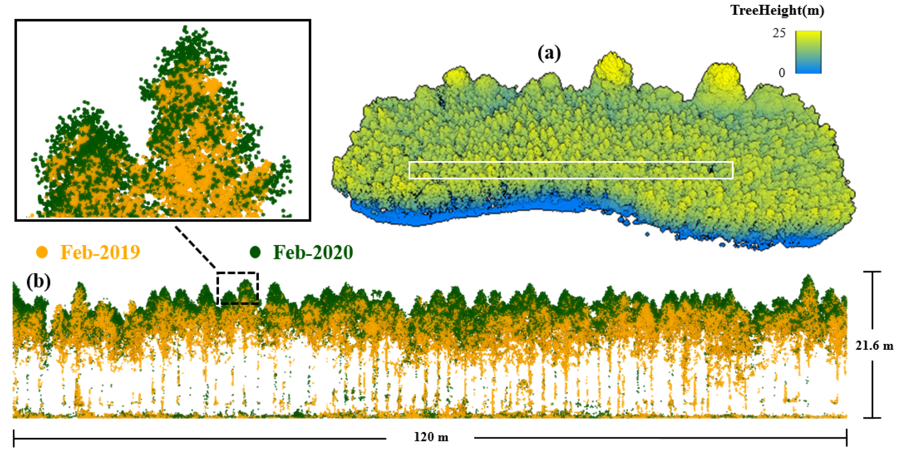
UAV–LiDAR data were collected using a SZT-R250 3D laser scanning system of the China Southern Surveying and Mapping Company. This system was equipped with the LiDAR equipment RIEGL miniVUX-1UAV for the DJI M600pro drone, with a pulse frequency of 100 kHz and a maximum measurement distance of 250 m. To ensure that the scanning results covered the entire research area and obtained clear tree contours, it was necessary to ensure sufficient point cloud density, laser pulse incidence zenith angle, and azimuth distribution as evenly as possible. The drone was set at an average altitude of 80 m, a scanning speed of 50 lines/s, and on a cross-plot route. The ground projection scanning width of each route was 120 m (60 m on both the left and right sides of the route), and the point cloud density was approximately 150–200 pts/m2 (Figure 3), which could record up to five returns. The study area was monitored in February 2019 and February 2020 with the data projection coordinates of the WGS 84/UTM. Synchronized with drones, the real-time kinematic positioning (RTK) base stations were installed at the same ground control points each time for static control measurements. Then, the point cloud data were decomposed based on the coordinate information of the fixed-point RTK static control measurements, reducing the coordinate error of the point cloud data and the system error between multitemporal data. The horizontal error was within 3 cm, and the vertical deviation between the hard-coverage control point and the multitemporal ground point cloud was controlled at approximately 5 cm (Figure 3) to ensure spatial consistency and comparability between the multitemporal data.

2.3. Field Data

From 2019 to 2020, the DBH of each tree in the study area was measured every February using calipers. DBH was classified into 2 cm intervals, and the standard trees were chosen as those closest to the average DBH of all trees within each grade. In February 2019, the height of 326 standard wooden trees were measured using an 18 m telescopic height measuring rod in conjunction with the Hawkeye HK-800 ranging telescope (with an accuracy of 0.1 m and a range of 3.5–800 m), and these standard trees were further divided into 166 for model building and 160 for sample validation. Aboveground biomass was calculated using an allometry equation suitable for this age group [27] (Table 1). Simultaneously, we measured the maximum contact height between 159 standard trees in the validation samples (removing one compressed tree that did not come into contact with surrounding trees) and the surrounding trees (four trees) in four directions—east, west, north, and south—and calculated the average maximum contact height. To match the spatial information of the sample plot boundary, ground survey data, and remote sensing data, the South Surveying and Mapping Galaxy 6 RTK real-time dynamic positioning technology was used to obtain the sample vertex and standard wood coordinates. The standard wood coordinates were adjusted based on the orthophoto image obtained using a DJI Phantom 4 RTK drone. Field investigations were conducted shortly after the LiDAR flight to reduce time differences.

2.4. UAV–LiDAR Data Processing

After denoising and classifying the point cloud into ground and non-ground points, Kriging interpolation was used to generate a Digital Surface Model for all point clouds, and irregular triangular network interpolation was used to generate a Digital Elevation Model (DEM). The CHM was calculated based on the difference between the two. Based on a previous study [22], we used a plot resolution of c = n , where n is the pulse density, and a CHM watershed segmentation algorithm to generate individual tree seed points (treetop coordinates) and crown bounding polygons. Subsequently, the vector image of the seed point was overlayed onto the orthophoto image (DJI Phantom 4 RTK drone) captured simultaneously with the point cloud data. Visual interpretation was then utilized to refine the seed points, involving the addition of undetected tree seed points and the removal of over-segmented points.
Using the DEM to normalize the point cloud (with the ground as the 0 elevation), combined with the modified seed point coordinates, individual tree point cloud segmentation was performed based on the distance discriminant clustering method between point clouds [19]. Finally, the tree height (TH) was obtained by extracting the maximum height coordinate from each crown point cloud, and the crown diameter (CD) was calculated as the diameter of the equal-area circle encompassing the crown polygon. The preprocessing of the point cloud and the extraction of parameters were accomplished using LIDAR360 5.0 software (Beijing Digital Green Earth Company, Beijing, China).

2.5. Effective Crown Area Extraction

To determine the ECA, the ECH must first be determined. Because the effective crown refers to the uncovered crown layer in the vertical direction that contributes most to photosynthesis [13,14], the ECH of Chinese fir plantations is the average maximum contact height. Considering the low efficiency of traditional ECH extraction, we extended two methods for automatically extracting it based on CHM segmentation and point cloud segmentation. Method 1 involves using the crown bounding polygons obtained by CHM watershed segmentation algorithm, and then the CHM pixel values located at the boundary are averaged to obtain ECH. Method 2 is based on the individual tree point cloud segmentation results, where each segmented tree point cloud was extracted and voxelized. Each voxel refers to a three-dimensional container used to encapsulate the point cloud (i.e., a 1 m × 1 m × 1 m rectangular cross-section) and then traverse all voxels on each tree. We assumed that if a voxel contained the point clouds of two or more trees, it was considered a tree-to-tree contact voxel. Multiple voxels may exist between trees as contact voxels, and the height of the contact voxel with the highest position was considered as the contact height (Figure 4b). ECH is the mean of all maximum contact heights around it (Figure 4a). To explore the impact of voxel height determination on ECH estimation, voxels at heights of 1, 0.50, 0.25, and 0.10 m were validated.
The ECH was determined using the optimal method between method 1 and method 2, and the point cloud above the height threshold was subsequently clipped. The ECA was calculated using the three-dimensional convex hull (Convex Hull). The aforementioned operations were implemented using the Scipy, Laspy, and Numpy modules of Python.

2.6. Biomass Dynamic Estimation

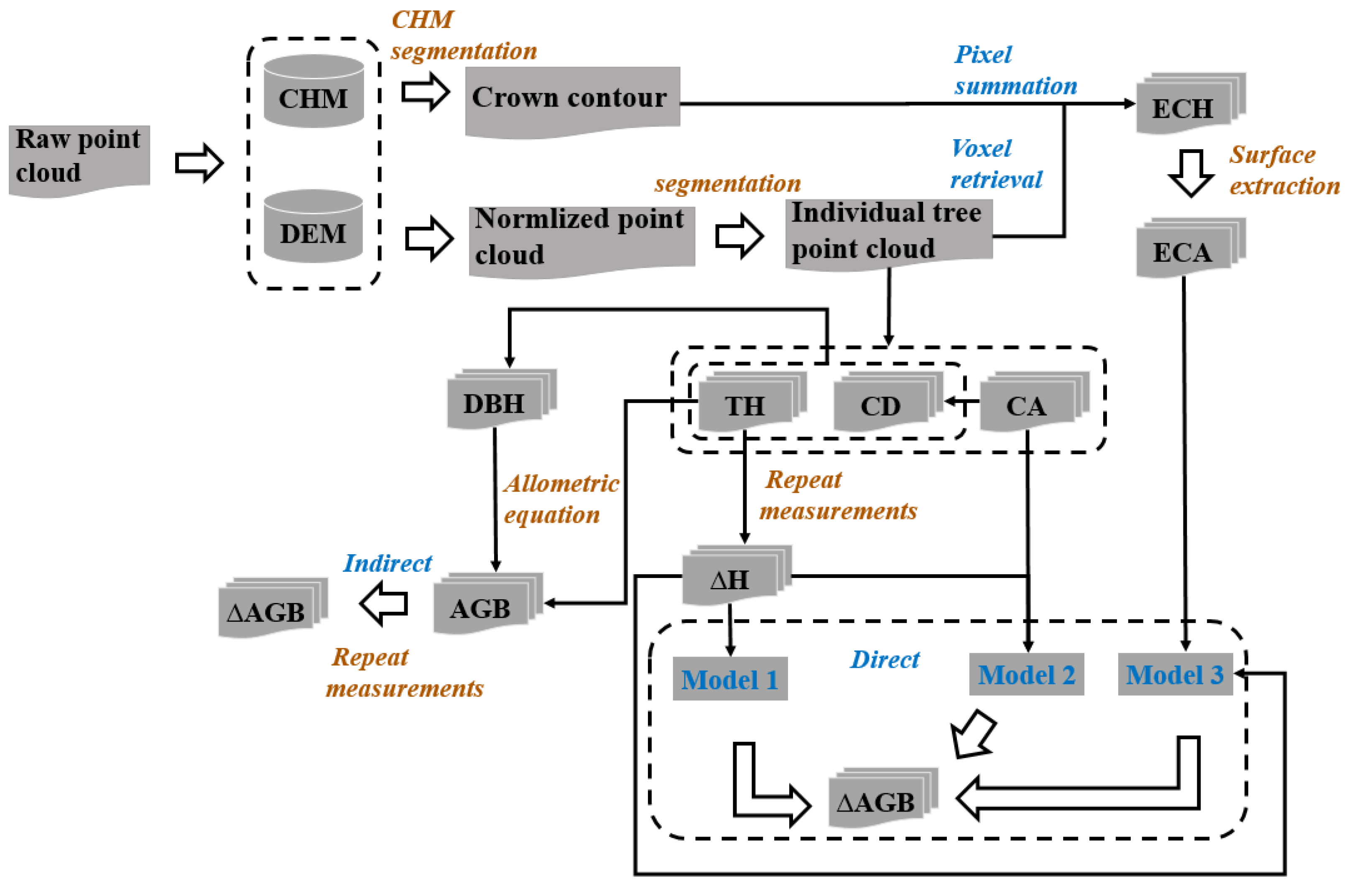
Direct and indirect methods were used to estimate biomass changes (∆AGB) in the Chinese fir plantations(Figure 5). A direct method refers to inverting structural parameters through two temporal LiDAR datasets, by calculating their differences as independent variables to estimate ∆AGB. The estimation model can be expressed in the following generalized form [9]:
B i = α 0 + k = 1 n β k x k i + ε i
where B i is the ground estimated change of AGB in the ith tree or plot, α 0 is the constant term, n is the total number of variables in the model, β k is coefficient estimated for independent variables, x k i is the differences between metrics (or “delta values”) in the ith tree or plot, and ε i is the error term [28]. We used three direct estimation models for single-tree ∆AGB using LiDAR parameters. Only the annual change in tree height (∆H) was used as a model parameter (Model 1) while the crown projection area (CA) and ∆H were used as parameters (Model 2). Considering the correlation between ECA and growth, a ∆AGB model (Model 3) was constructed using ∆H and ECA. Based on 166 standard trees located in the research area, a linear model was fitted separately and a 5-fold cross-validation was used.
An indirect method uses independent models for each period to estimate AGB at two time points (2019 and 2020 in our case) and calculates the difference between the two estimates to quantify changes in AGB. The general form of the AGB estimation model for a single time is as follows:
B i t = α 0 t + k = 1 n β k t x k i t + ε i t
where B i t is the ground estimated AGB at one time point (t = the year of 2019 or 2020 in our case) in the ith tree or plot and x k i t is the derived metrics at one time point [9]. Finally, B i is calculated as the difference between B i 2019 and B i 2020 . Considering the importance of the DBH in the allometry equation, and the inability of the “top-down” scanning of UAV–LiDAR to directly obtain the trunk information, two independent variables, namely, TH and CD, were extracted after the single-tree segmentation of point clouds, and then a regression model was constructed to estimate DBH, and then DBH and TH were substituted into Table 1 allometry equation to calculate AGB. The aforementioned operations were implemented using the Python. Individual tree-scale structural parameter testing and comparison of the direct and indirect methods were conducted using additional 160 standard trees.

2.7. Precision Verification and Statistical Analysis

An individual tree segmentation accuracy adopting F-score, Precision (P), and Recall (Re) was evaluated using three indicators [19], where a lower Re value indicates a higher number of misclassified plants, indicating excessive segmentation; the lower the value of p, the more missing branches there are, and the CHM is under segmentation; and F-score represents the overall accuracy of considering missed and misclassified trees. The formula is as follows:
R e = N t N t + N c
P = N t N t + N o
F _ s c o r e = 2 ( P × R ) P + R
where N t refers to the trees correctly detected, N o refers to the trees undetected, and   N c refers to the trees falsely detected.
The reliability and functional fitting effect of the parameter and growth estimation were evaluated based on the coefficient of determination (R2), root-mean-squared error (RMSE), relative root-mean-squared error (rRMSE), and bias (Bias).
R 2 = i = 1 n ( P i P ¯ ) ( Q i Q ¯ ) i = 1 n ( P i P ¯ ) 2 i = 1 n ( P i P ¯ ) 2 2
R M S E = i = 1 n ( P i Q i ) 2 n
r R M S E = R M S E Q ¯
B i a s = i = 1 n ( Q i P i ) n
where P i and Q i represent the predicted and observed values; P ¯ and Q ¯ indicate the mean values; and n denotes the total alive trees in a sample plot.

3. Results

3.1. Verification of Individual tree Segmentation Accuracy

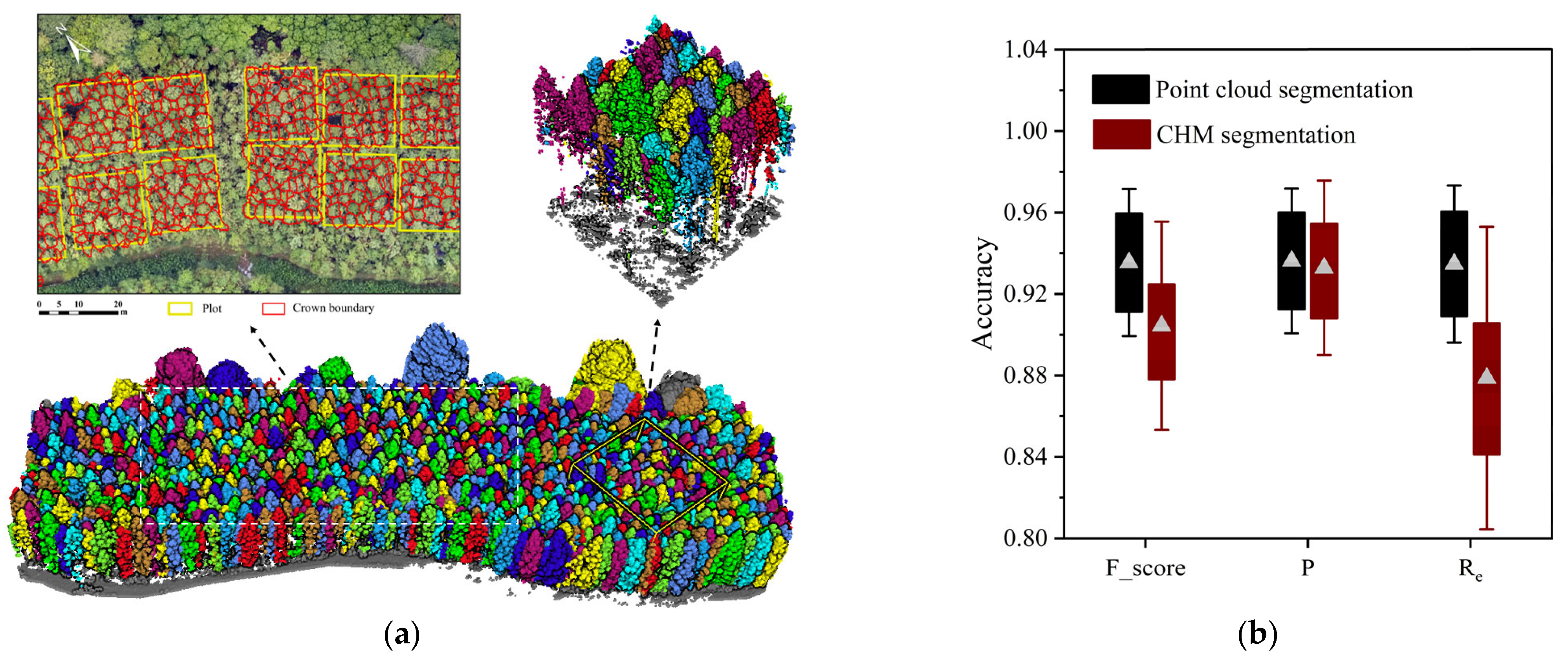
Individual tree recognition was the basis for estimating single-tree structural parameters in this study. Point cloud segmentation was performed based on the manually assisted correction of the tree coordinate seed points. In this study, the middle-aged Chinese fir plantation achieved a high single-tree segmentation accuracy (Figure 6b), the average total accuracy (F-score) of single-tree segmentation for the 16 samples was 0.93, and Re and p were also 0.93 and 0.92, respectively. Except for one outlier in Re, the lowest values of the three precision indices were greater than 0.85. The segmentation accuracy of CHM segmentation method was slightly worse than that of a single-point cloud method, with an average F-score of 0.90, p of 0.92, and Re value of 0.88.

3.2. Validation of Effective Crown Height

In method 2, setting different voxel heights had a significant impact on the accuracy of ECH, and as the voxel height decreased, the accuracy gradually increased. The accuracy at a height of 0.10 m voxel was the highest (RMSE = 0.58 m, rRMSE = 3.98%, Bias = 0.29 m), followed by the accuracy at voxel heights of 0.25 m (RMSE = 0.62 m, rRMSE = 4.26%, Bias = 0.36 m), 0.50 m (RMSE = 0.73 m, rRMSE = 4.97%, Bias = 0.47 m), and finally 1.00 m (RMSE = 0.89 m, rRMSE = 6.09%, Bias = 0.72 m). The accuracy of ECH extraction improves with decreasing voxel height. However, a continuous reduction in the number of common point clouds between adjacent plants occurs as well. When the voxel height decreases to 0.1 m, the contact height extracted from point cloud between plants cannot be acquired, leading to ECH missing the results of three plants (N dropped from 159 to 156). The optimal voxel size for this study was 1 m × 1 m × 0.25 m (Table 2).
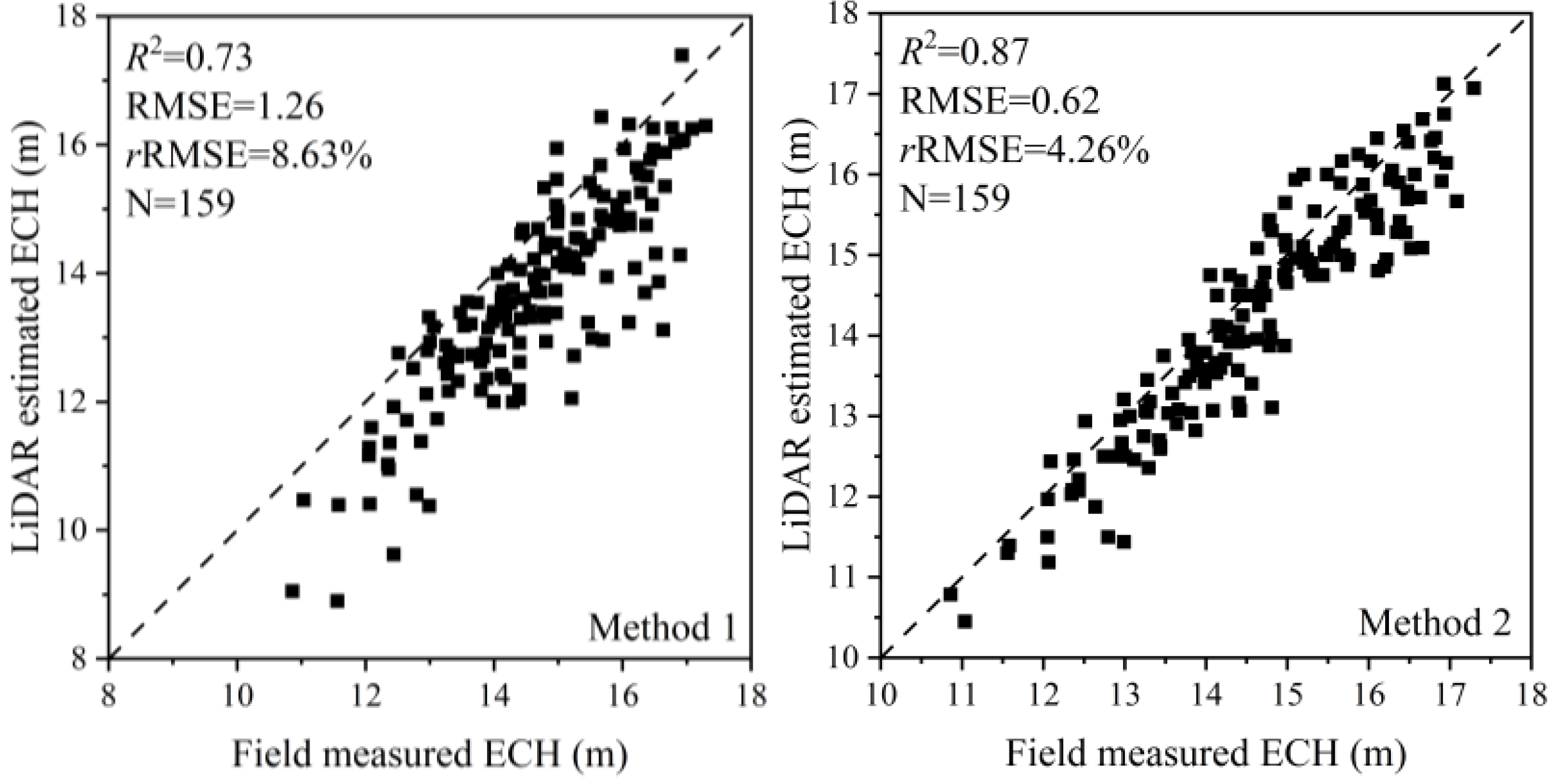
Method 1 extracted the ECH with an accuracy of R2 = 0.73, RMSE = 1.26 m, and rRMSE = 8.63%, resulting in a significant degree of underestimation. It can be seen that method 2 has better results than method 1 (Figure 7).

3.3. Verification of Structural Parameter Estimation

The TH and CD parameters were obtained directly from point cloud single-tree segmentation. The two parameters were used as independent variables, and a regression equation was used to estimate DBH (Equation (10)). The model has been validated through the F-test, further confirming its favorable goodness-of-fit, with an F-value of 248.96 and p < 0.01.
D B H = 0.86 T H + 1.92 C D 1.11
where DBH is the diameter at breast height, TH is the tree height, and CD is the crown diameter.
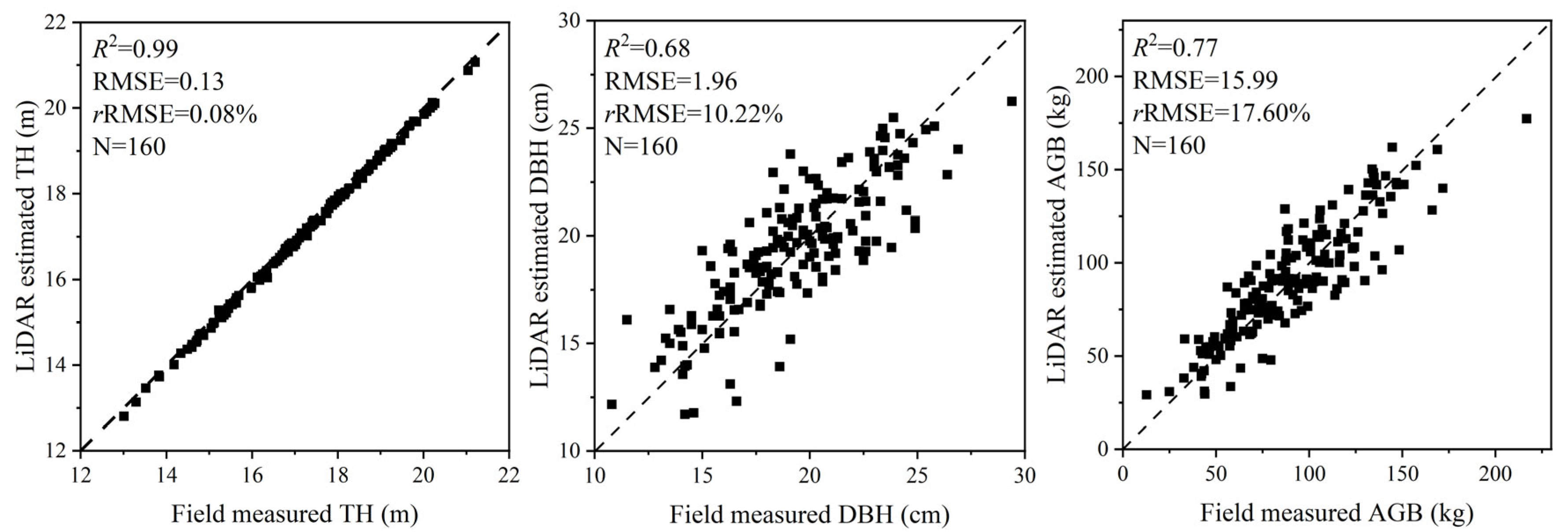
A comparison of the estimated results of the structural parameters with the field measurements (Figure 8) shows that all parameters had an estimated R2 > 0.65. Among them, the accuracy of TH monitoring was the highest (R2 = 0.99, RMSE = 0.13 m, rRMSE = 0.08%), followed by AGB (R2 = 0.77, RMSE = 15.99 kg, rRMSE = 17.60%), and DBH (R2 = 0.68, RMSE = 1.96 cm, rRMSE = 10.22%).

3.4. Analysis of Growth from Biomass Changes

The correlation analysis showed that the coefficient of determination R2 between ECA and the field measured ∆AGB is 0.47 and the p-value is less than 0.01 (Figure 9). There was a strong correlation between these two parameters. Three parameter selection methods were used to establish a direct estimation model for AGB. Among them, Model 1 only used ∆H as the input parameter, and the fitting effect of the model was relatively poor (R2 = 0.33, p < 0.01). Model 2, with the introduction of CA, had a significantly improved the model fitting effect, with R2 increasing to 0.57. Furthermore, Model 3, which replaced CA with ECA, achieved the best fitting effect. R2 is 0.63, indicating the high reliability of the model (Table 3).
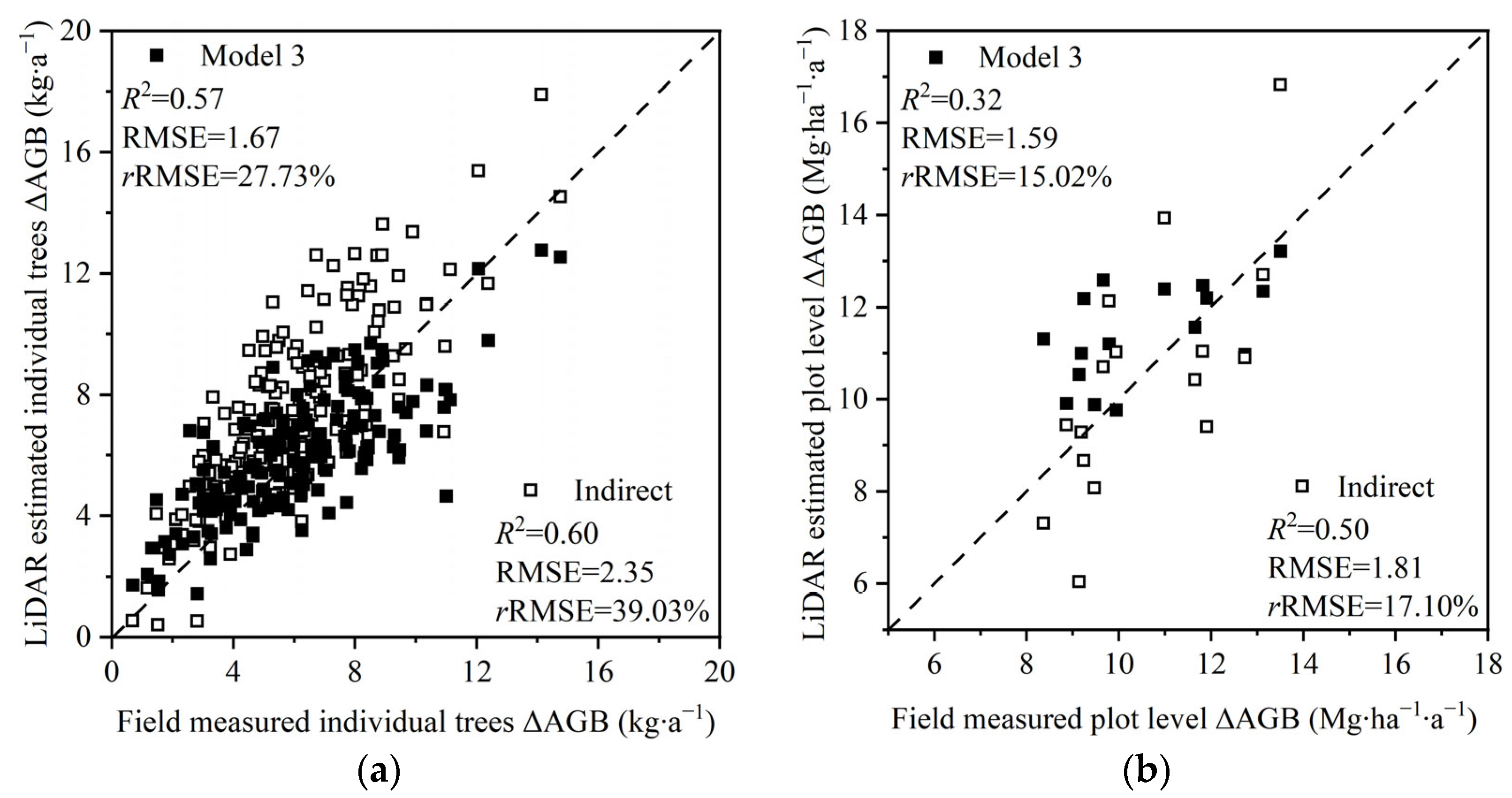
Furthermore, Model 3 and the indirect method were compared. The results showed that Model 3 had a similar performance to the indirect method at both the individual tree and plot scales. At the single-tree scale, the RMSE of the direct method was 1.67 kg∙a−1, and rRMSE was 27.73%, while the indirect method had an RMSE of 2.35 kg∙a−1 and an rRMSE of 39.03% (Figure 10a). However, R2 (0.57) of the direct method was lower than that (0.60) of the indirect method. After calculating the biomass per unit area, the relative errors of both methods decreased, with the direct method having an rRMSE of 15.02%, and the indirect method having an rRMSE of 17.10% (Figure 10b). At the plot level, R2 (0.32) of the direct method is also lower than that (0.50) of the indirect method.
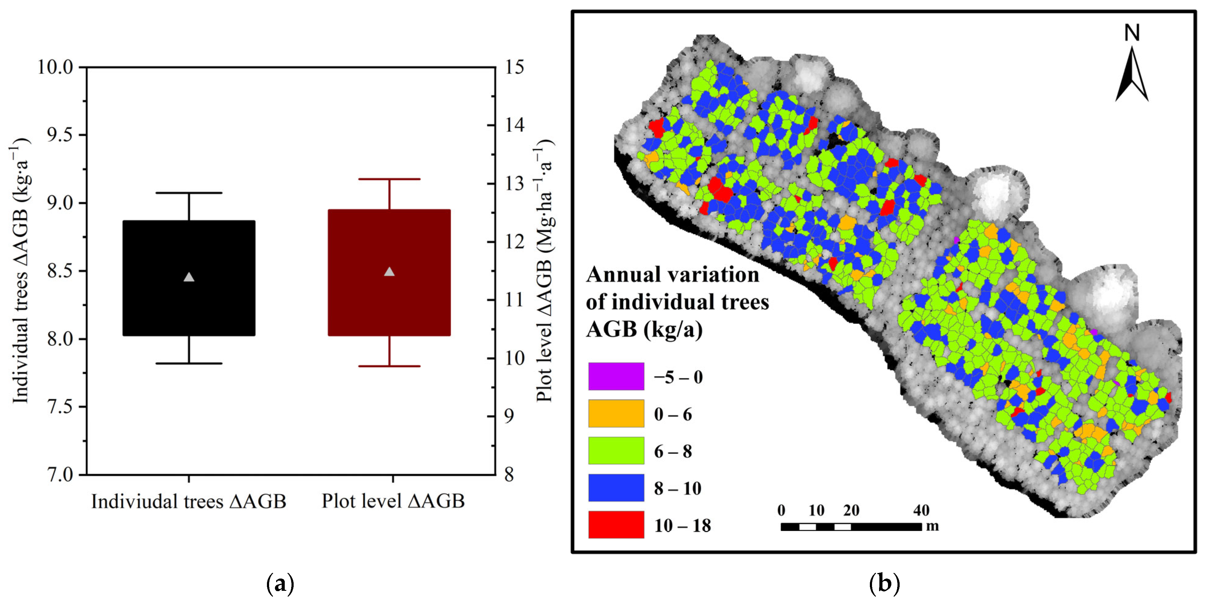
The monitoring results of the two-temporal LiDAR indicated that the average annual growth of individual AGB of the 17-year-old Chinese fir plantations from 23 February 2019 to 25 February 2020 was 8.45 kg∙a−1, and the annual growth rate of biomass density was 11.47 Mg∙ha−1∙a−1 (Figure 11a).

4. Discussion

4.1. Effective Crown Extraction

Locating the effective crown positions of individual trees and extracting effective crown information may be key steps in using LiDAR for estimating forest growth and carbon sequestration. This study used UAV–LiDAR to extract the effective crowns of Chinese fir plantations using the maximum contact height of individual trees as the threshold. Previous studies have attempted different methods for locating effective crowns. The effective crown height of larch (Larix olgensis) plantations is approximately equal to the average contact height of the stand [14]. Alternatively, it can be determined as the height corresponding to 90% of the relative accumulated leaf biomass [24]. For Korean pine (Pinus koraiensis) plantations, it is determined by the height of tree knots [18]. Remote sensing technology has also been employed for the determination of ECH. Geng et al. [29] used airborne LiDAR to generate a CHM based on a marker-controlled watershed algorithm to extract the average maximum contact height as the ECH, thereby drawing an effective coronal 3D map. From the perspective of dendrology, determining the effective crown height is the most accurate method; however, large-scale sampling requires intensive labor. Despite certain biases, locating and extracting effective crown information based on UAV–LiDAR can replace traditional manual surveys to a certain extent and can also be more widely applied on a regional or larger scale. This study further compared two methods for extracting ECH based on UAV–LiDAR and found that method 2 was superior to method 1. Individual tree segmentation is a prerequisite for effective crown extraction, and based on CHM watershed segmentation, two-dimensional crown contours can be directly obtained. Additionally, it is possible to determine the coordinates of the tree top, supplemented by a manual revision of the coordinates, to reduce misidentification and missed recognition rates, and improve the accuracy of single-tree 3D point cloud segmentation [19], which is crucial for further calculating ECH.
Extracting the ECH based on a single-tree point cloud, which determines the average maximum contact height between individual trees, requires the size of the voxels to be determined. The flat voxel shape increases the probability of including inter-plant point clouds and helps refine the height stratification. Consequently, referring to the crown radius, we set the length of the top and bottom edges to 1 m and compared the impact of voxel resolution at different heights on ECH extraction, ultimately determining the optimal voxel size of 1 m × 1 m × 0.25 m. We found significant differences in the point cloud attributes obtained by the different LiDAR sensors as well as differences in the extracted canopy parameters and optimal voxel sizes. Zheng et al. [30] conducted a sensitivity analysis of the directional gap fraction of the voxel size (0.1–26 m), and the results showed that voxel size is a key factor in estimating the directional gap fraction using LiDAR data. Similarly, in the determination of canopy height, the voxel size is influenced by the point density. Wang et al. [31] utilized a point cloud dataset with a density of 4.1 points per square meter to extract the forest canopy height. By setting a voxel height of 0.15 m and comparing it with voxels ranging from 10 to 40 m in horizontal size, the study revealed that the voxel with a horizontal size of 18 m achieved the highest extraction accuracy. In summary, the optimal voxel size may vary depending on the research objective and field. Therefore, the optimal voxel size should be determined based on the specific vegetation types, tree density, estimated parameters, laser pulse density, terrain, and other factors.

4.2. Comparison of Forest Annual Growth Estimation by Direct and Indirect Methods

Long-term repeated monitoring using LiDAR helps to understand the development of crown structure and growth. Besides ΔH, we observed that the ECA had a greater impact than the CA on predicting the growth of individual Chinese fir. ECA is proportional to the crown surface area that receives solar radiation and hence provides a link to tree growth [17]. However, tree growth is also influenced by other environmental conditions such as temperature and soil moisture. Consequently, the structural parameters of ECA and ΔH are insufficient for the accurate determination of tree growth, resulting in a partial fraction (37%) of tree growth variance that remains unexplained by the structural parameters (Table 2). This study primarily emphasizes the significance of the ECA in predicting annual growth. However, the ECA is more applicable to single-age plantations; its suitability diminishes for mixed forests or secondary broad-leaved forests due to the limited accuracy of individual tree point cloud segmentation, which directly influences the precise extraction of the ECA parameter. Alternatively, if the extraction of the ECA is conducted at the plot level, the vertical distribution characteristics of the leaf area density can be obtained based on the point cloud penetration rate and Beer’s law. Subsequently, the ECH can be determined, allowing the realization of the fitting surface area and extraction of the plot-level ECA.
The comparison of direct and indirect methods for estimating plot level ΔAGB revealed that the accuracy of the direct method (RMSE = 1.59 Mg∙ha−1∙a−1, rRMSE = 15.02%) was slightly higher than that of the indirect method (RMSE = 1.81 Mg∙ha−1∙a−1, rRMSE = 17.10%). This is consistent with the viewpoint of Bollandsås et al., who hypothesized that a direct method is only affected by errors in one model rather than in two models [9]. Cao et al. [8] calculated the biomass dynamics of Yushan Forest in Jiangsu Province, China, over a period of six years based on airborne LiDAR data collected at two time points. The direct method had a better accuracy, with an RMSE of 2.91 Mg∙ha−1∙a−1 and rRMSE of 25.64%. Økseter et al. [10] estimated the biomass change of forests over an 11-year period in southeastern Norway using ALS data collected at two time points, with an indirect estimation method of an rRMSE of only 14.8%. Existing research focused on growth dynamics spanning three years or longer [1,8,32]. Owing to the limitations of LiDAR sensor accuracy, the relative error of growth in a shorter period is larger, leading to an increased uncertainty in monitoring growth changes [32]. Andersen et al. [33] confirmed that airborne LiDAR can monitor growth changes over a period of fewer than 2 years. Despite the presence of some errors in forest growth estimation, the effective crown information extracted based on UAV–LiDAR and multitemporal monitoring has proven to be an essential supplement to traditional forest inventory, and can provide valuable reference materials for producing plantation productivity maps with a higher resolution than sample plots.

5. Conclusions

This research focused on a 17-year-old Chinese fir plantation as the subject of investigation. A UAV–LiDAR system was employed to acquire discrete point cloud data, while concurrent ground-based measurements of individual tree parameters were conducted. After a comprehensive comparison of two effective crown height (ECH) algorithms, the most optimal one was selected for the further computation of the individual tree’s effective crown area (ECA). Subsequently, we explored the implications of incorporating ECA into a regression model to enable the direct prediction of the annual AGB growth. Finally, a comparative analysis was performed to evaluate the efficacy of the direct and indirect methods in predicting the annual dynamics of AGB. The study resulted in three main conclusions:
(1)
Compared with the canopy boundary height average method based on CHM segmentation, the voxel extraction method based on normalized point cloud segmentation can obtain a more accurate ECH. However, the accuracy of ECH extraction was influenced by the voxel size setting. Referring to the average tree crown radius, the horizontal plane of the voxel was set to 1 m × 1 m, and the optimal voxel height was determined to be 0.25 m.
(2)
The ECA was a crucial factor for accurately estimating the annual growth of Chinese fir plantations. Moreover, ECA exerts a more significant influence than CA on enhancing the fitting effect of the annual growth regression model.
(3)
The use of multi-temporal UAV–LiDAR allows for the reliable and efficient monitoring of AGB in Chinese fir plantations, including its annual changes. The regression model, which incorporates two variables: ECA and ∆TH, was superior to the indirect method for annual growth estimation. By assessing the AGB and its variation from individual plant to plot level, a reduction in relative error was observed.

Author Contributions

Methodology, software, validation, formal analysis, H.Z. and J.X.; investigation, H.Z., J.X., G.C. and Y.L.; writing—original draft preparation, writing—review and editing, J.X. and H.Z.; supervision, project administration, funding acquisition, J.M.C., H.Z. and G.M. All authors have read and agreed to the published version of the manuscript.

Funding

This research was funded by the National Key Research and Development Program of China (grant number 2020YFA0608701), Fujian Science and Technology Plan Guidance Project (grant number 2022L3009), Fujian Provincial Public Welfare Research Institute Basic Research Project (grant number 2023R11010007-6).

Data Availability Statement

Data sharing is not applicable to this article.

Acknowledgments

The authors would like to express appreciation for the support provided by researchers Li Xiaojie and Lv Maokui from Fujian Normal University during the field investigation of this study.

Conflicts of Interest

The authors declare no conflict of interest.

References

  1. Dubayah, R.O.; Sheldon, S.L.; Clark, D.B.; Hofton, M.A.; Blair, J.B.; Hurtt, G.C.; Chazdon, R.L. Estimation of tropical forest height and biomass dynamics using lidar remote sensing at La Selva, Costa Rica. J. Geophys. Res. Biogeosci. 2010, 115, G00E09. [Google Scholar] [CrossRef]
  2. Houghton, R.A.; Goetz, S.J. New Satellites Help Quantify Carbon Sources and Sinks. Eos Trans. Am. Geophys. Union 2008, 89, 417–418. [Google Scholar] [CrossRef]
  3. Clark, D.A. Tropical forests and global warming: Slowing it down or speeding it up? Front. Ecol. Environ. 2004, 2, 73–80. [Google Scholar] [CrossRef]
  4. Liu, H.; Zhang, Z.N.; Cao, L. Estimating forest stand characteristics in a coastal plain forest plantation based on vertical structure profile parameters derived from ALS data. Natl. Remote Sens. Bull. 2018, 22, 872–888. (In Chinese) [Google Scholar] [CrossRef]
  5. Guo, Q.H.; Liu, J.; Tao, S.L.; Xue, B.L.; Li, L.; Xu, G.C.; Li, W.K.; Wu, F.F.; Li, Y.M.; Chen, L.H. Application status and Prospect of lidar in forest ecosystem monitoring and simulation. Chin. Sci. Bull. 2014, 56, 20. (In Chinese) [Google Scholar]
  6. Marinelli, D.; Paris, C.; Bruzzone, L. A Novel Approach to 3-D Change Detection in Multitemporal LiDAR Data Acquired in Forest Areas. Ieee Trans. Geosci. Remote Sens. 2018, 56, 3030–3046. [Google Scholar] [CrossRef]
  7. Næsset, E.; Bollandsås, O.M.; Gobakken, T.; Gregoire, T.G.; Ståhl, G. Model-assisted estimation of change in forest biomass over an 11year period in a sample survey supported by airborne LiDAR: A case study with post-stratification to provide “activity data”. Remote Sens. Environ. 2013, 128, 299–314. [Google Scholar] [CrossRef] [Green Version]
  8. Cao, L.; Coops, N.C.; Innes, J.L.; Sheppard, S.R.J.; Fu, L.; Ruan, H.; She, G. Estimation of forest biomass dynamics in subtropical forests using multi-temporal airborne LiDAR data. Remote Sens. Environ. 2016, 178, 158–171. [Google Scholar] [CrossRef]
  9. Bollandsås, O.M.; Gregoire, T.G.; Næsset, E.; Øyen, B.-H. Detection of biomass change in a Norwegian mountain forest area using small footprint airborne laser scanner data. Stat. Methods Appl. 2012, 22, 113–129. [Google Scholar] [CrossRef]
  10. Økseter, R.; Bollandsås, O.M.; Gobakken, T.; Næsset, E. Modeling and predicting aboveground biomass change in young forest using multi-temporal airborne laser scanner data. Scand. J. For. Res. 2015, 30, 458–469. [Google Scholar] [CrossRef]
  11. McRoberts, R.E.; Næsset, E.; Gobakken, T.; Bollandsas, O.M. Indirect and direct estimation of forest biomass change using forest inventory and airborne laser scanning data. Remote Sens. Environ. 2015, 164, 36–42. [Google Scholar] [CrossRef]
  12. Kato, A.; Moskal, L.M.; Schiess, P.; Swanson, M.E.; Calhoun, D.; Stuetzle, W. Capturing tree crown formation through implicit surface reconstruction using airborne lidar data. Remote Sens. Environ. 2009, 113, 1148–1162. [Google Scholar] [CrossRef]
  13. Kajihara, M. Estimation of stem-volume increment by using sunny crown-surface area and stem-surface area. J. Jpn. Soc. 2008, 67, 501–505. [Google Scholar]
  14. Li, F.R.; Wang, Z.F. Studies on the effective crowndevelopment of larix olgensis (I)—Determination of the effective crown. J. Northeast For. Univ. 1996, 24, 1–8. (In Chinese) [Google Scholar]
  15. Mller, C.M. The influence of pruning on the growth of conifers. Forestry 1962, 33, 37–53. [Google Scholar] [CrossRef]
  16. Liu, Q.; Xie, L.; Dong, L.; Li, F. Dynamic simulation of the multilayer crown net photosynthetic rate and determination of the functional crown for larch (Larix olgensis) trees. New For. 2021, 52, 1011–1035. [Google Scholar] [CrossRef]
  17. Zheng, Y.; Jia, W.; Wang, Q.; Huang, X. Deriving individual-tree biomass from effective crown data generated by terrestrial laser scanning. Remote Sens. 2019, 11, 2793. [Google Scholar] [CrossRef] [Green Version]
  18. Zhu, W.; Liu, Z.; Jia, W.; Li, D. Modelling the Tree Height, Crown Base Height, and Effective Crown Height of Pinus koraiensis Plantations Based on Knot Analysis. Forests 2021, 12, 1778. [Google Scholar] [CrossRef]
  19. Li, W.; Guo, Q.; Jakubowski, M.K.; Kelly, M. A New Method for Segmenting Individual Trees from the Lidar Point Cloud. Photogramm. Eng. Remote Sens. 2012, 78, 75–84. [Google Scholar] [CrossRef] [Green Version]
  20. Nunes, M.; Ewers, R.; Turner, E.; Coomes, D. Mapping Aboveground Carbon in Oil Palm Plantations Using LiDAR: A Comparison of Tree-Centric versus Area-Based Approaches. Remote Sens. 2017, 9, 816. [Google Scholar] [CrossRef] [Green Version]
  21. Popescu, S.C.; Wynne, R.H.; Nelson, R.F. Measuring individual tree crown diameter with lidar and assessing its influence on estimating forest volume and biomass. Can. J. Remote Sens. 2003, 29, 564–577. [Google Scholar] [CrossRef]
  22. Chen, Q.; Baldocchi, D.; Gong, P.; Kelly, M. Isolating Individual Trees in a Savanna Woodland Using Small Footprint Lidar Data. Photogramm. Eng. Remote Sens. 2006, 72, 923–932. [Google Scholar] [CrossRef] [Green Version]
  23. Ma, K.; Chen, Z.; Fu, L.; Tian, W.; Jiang, F.; Yi, J.; Du, Z.; Sun, H. Performance and Sensitivity of Individual Tree Segmentation Methods for UAV-LiDAR in Multiple Forest Types. Remote Sens. 2022, 14, 298. [Google Scholar] [CrossRef]
  24. Bai, D.X.; Liu, Q.; Dong, L.H.; Li, F.R. Determination and analysis of height to effective crown for planted Larix olgensis trees. J. Beijing For. Univ. 2019, 41, 76–87. (In Chinese) [Google Scholar]
  25. Zhang, X.; Duan, A.; Zhang, J. Tree biomass estimation of Chinese fir (Cunninghamia lanceolata) based on Bayesian method. PLoS ONE 2013, 8, e79868. [Google Scholar] [CrossRef] [Green Version]
  26. Department Of Forest Resources Management S.F.A. The 7th National forest inventory and status of forest resources. For. Resour. Manag. 2010, 1, 1–8. (In Chinese) [Google Scholar]
  27. Qian, N.Z.; Ye, J.Z. Biomass of Chinese fir mixed family plantation in Yangkou forest farm. J. Nanjing For. Univ. Nat. Sci. 1992, 16, 6. (In Chinese) [Google Scholar]
  28. Bollandsås, O.M.; Næsset, E. Using delta values of multi-temporal first-return small footprint airborne laser scanner data to predict change of tree biomass in mountain spruce forests. Silvilaser 2010, 9, 411–417. [Google Scholar]
  29. Geng, L.; Li, M.Z.; Fan, W.Y.; Wang, B. Individual Tree Structure Parameters and Effective Crown of the Stand Extraction Base on Airborn LiDAR Data. Sci. Silvae Sin. 2018, 54, 11. (In Chinese) [Google Scholar]
  30. Zheng, G.; Ma, L.; Eitel, J.; Wei, H.; Magney, T.S.; Moskal, L.M.; Li, M. Retrieving directional gap fraction, extinction coefficient, and effective leaf area index by incorporating scan angle information from discrete aerial lidar data. IEEE Trans. Geosci. Remote Sens. 2016, 55, 577–590. [Google Scholar] [CrossRef]
  31. Wang, C.; Luo, S.; Xi, X.; Nie, S.; Ma, D.; Huang, Y. Influence of voxel size on forest canopy height estimates using full-waveform airborne lidar data. For. Ecosyst. 2020, 7, 12. [Google Scholar] [CrossRef]
  32. Zhao, K.; Suarez, J.C.; Garcia, M.; Hu, T.; Wang, C.; Londo, A. Utility of multitemporal lidar for forest and carbon monitoring: Tree growth, biomass dynamics, and carbon flux. Remote Sens. Environ. 2018, 204, 883–897. [Google Scholar] [CrossRef]
  33. Andersen, H.E.; Reutebuch, S.E.; McGaughey, R.J.; d’Oliveira, M.V.N.; Keller, M. Monitoring selective logging in western Amazonia with repeat lidar flights. Remote Sens. Environ. 2014, 151, 157–165. [Google Scholar] [CrossRef] [Green Version]
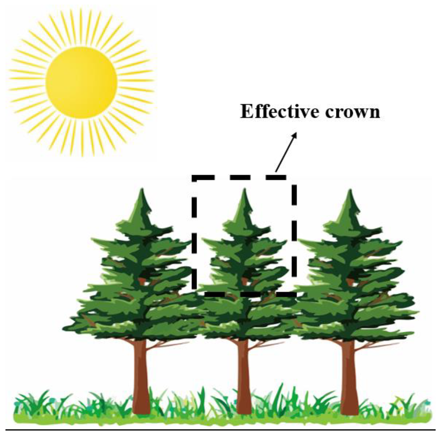
Figure 1. Schematic diagrams of effective crown.
Remotesensing 15 03869 g001
Figure 2. Location of the study area, which (a) showcases the location of the research area of Fujian Province, China, and (b) shows the positions of all 18 m × 18 m Chinese fir plantation plots nested on an orthophoto image of the study area (WGS 84/UTM zone 50N).
Remotesensing 15 03869 g002
Figure 3. LiDAR point cloud profile, in which (a) is the 3D point cloud in the research area and (b) is the double time point cloud profiles, with a section length of 120 m and a width of 2 m.
Remotesensing 15 03869 g003
Figure 4. Principle of method 2 for locating and extracting effective coronary information. Among them, (a) is the orthophoto distribution map of trees around the target tree. Each distinct-colored point cloud represents an individual tree, obtained through segmentation and identification. The labels ①, ②, ③, and ④ are employed in a clockwise fashion to indicate neighboring trees in proximity to the target tree. (b) is the determination of the maximum contact height of the target tree in the profile based on the voxel method.
Remotesensing 15 03869 g004
Figure 5. Flow chart for estimating annual tree growth (∆AGB) using multitemporal UAV–LiDAR. CHM and DEM are the canopy height and the Digital Elevation models, respectively; ECH is the effective crown height; ECA is the effective crown area; CA is the projected area of the crown; CD is the crown diameter; TH is the tree height; AGB represents aboveground biomass; DBH is the diameter at breast height; ∆AGB and ∆H represent the annual changes in biomass and tree height, respectively; Model 1, Model 2, and Model 3 represent three parameter combination methods for the direct estimation of biomass change.
Remotesensing 15 03869 g005
Figure 6. Two algorithms for individual tree segmentation, where (a) is the display of individual tree segmentation results, and (b) is the box diagram of individual tree segmentation accuracy.
Remotesensing 15 03869 g006
Figure 7. The correlation scatter plot of method 1 by watershed segmentation and method 2 by point cloud segmentation. The legend represents the coefficient of determination (R2), root-mean-squared error (RMSE), relative root-mean-squared error (rRMSE), and the number of validation samples (N) between the observed and predicted values. Diagonal lines represent a perfect match between observed and predicted values.
Remotesensing 15 03869 g007
Figure 8. The correlation scatter plot of TH, DBH, and AGB. The legend represents the coefficient of determination (R2), root-mean-squared error (RMSE), relative root-mean-squared error (rRMSE), and the number of validation samples (N) between the observed and predicted values. Diagonal lines represent a perfect match between observed and predicted values.
Remotesensing 15 03869 g008
Figure 9. Scatter plot of the relationship between ECA and annual ∆AGB, where R2 represents the correlation coefficient, and p-value represents the significance of the correlation. A value less than 0.01 indicates a highly significant correlation between the two.
Remotesensing 15 03869 g009
Figure 10. The correlation scatter plot of Model 3 and indirect method at (a) individual tree level and (b) plot level. The legend represents the coefficient of determination (R2), root-mean-squared error (RMSE), and relative root-mean-squared error (rRMSE) between the observed and predicted values. Diagonal lines represent a perfect match between observed and predicted values.
Remotesensing 15 03869 g010
Figure 11. The growth rate of middle-aged Chinese fir, where (a) is the box diagram of ∆AGB in two temporal phases, and (b) is the individual tree growth changes in the study area.
Remotesensing 15 03869 g011
Table 1. Allometric biomass equations.
EquationR2
y t r u n k = 0.0407 D 1.5228 H 1.0703 0.978
y b r a n c h = 0.0226 D 3.1427 H 1.2466 0.854
y l e a f = 0.1354 D 2.9235 H 1.6995 0.842
y = y t r u n k + y b r a n c h + y l e a f
Where y represents aboveground biomass, D represents diameter at breast height, H represents tree height, and y t r u n k , y b r a n c h ,   a n d   y l e a f refer to the biomass of tree trunk, branches, and leaves, respectively.
Table 2. Verification of ECH accuracy extracted at different voxel heights.
Voxel Height (m)R2RMSE (m)Bais (m)rRMSEN
1.000.860.890.726.09%159
0.500.850.730.474.97%159
0.250.870.620.364.26%159
0.100.870.580.293.98%156
Table 3. Comparison of fitting effects of three direct estimation models for ∆AGB.
ModelEquationR2N
1 A G B = 6.71 H + 1.53 0.33166
2 A G B = 0.30 C A + 4.35 H + 1.52 0.57166
3 A G B = 0.09 E C A + 4.08 H + 0.93 0.63166
Where ∆AGB is the annual change in aboveground biomass, ∆H is the annual change in tree height, and ECA is the effective crown area.
Disclaimer/Publisher’s Note: The statements, opinions and data contained in all publications are solely those of the individual author(s) and contributor(s) and not of MDPI and/or the editor(s). MDPI and/or the editor(s) disclaim responsibility for any injury to people or property resulting from any ideas, methods, instructions or products referred to in the content.