A Novel Approach to Characterizing Crown Vertical Profile Shapes Using Terrestrial Laser Scanning (TLS)

Abstract

Crown vertical profiles (CVP) play an essential role in stand biomass and forest fire prediction. Traditionally, due to measurement difficulties, CVP models developed based on a small number of individual trees are not convincing. Terrestrial laser scanning (TLS) provides new insights for researching trees’ CVPs. However, there is a limited understanding of the ability to accurately describe CVPs with TLS. In this study, we propose a new approach to automatically extract the crown radius (CR) at different heights and confirm the correctness and effectiveness of the proposed approach with field measurement data from 30 destructively harvested sample trees. We then applied the approach to extract the CR from 283 trees in 6 sample plots to develop a two-level nonlinear mixed-effects (NLME) model for the CVP. The results of the study showed that the average extraction accuracy of the CR when the proposed approach was applied was 90.12%, with differences in the extraction accuracies at different relative depths into the crown (RDINC) ranges. The TLS-based extracted CR strongly correlated with the field-measured CR, with an R² of 0.93. Compared with the base model, the two-level NLME model has significantly improved the prediction accuracy, with R_a² increasing by 13.8% and RMSE decreasing by 23.46%. All our research has demonstrated that TLS has great potential for accurately extracting CRs, which would provide a novel way to nondestructively measure the crown structure. Moreover, our research lays the foundation for the future development of CVP models using TLS at a regional scale.

1. Introduction

The crown vertical profile (CVP) of a tree is the minimum boundary surrounding the crown that connects the tree top and the branch vertices [1]. It reflects the shape and size of the crown and directly describes peoples’ overall impression of a tree. The CVP has become one of the most critical forest structure parameters, both at the sample plot and tree levels, and it lays the foundation for exploring the spatial attributes of tree crowns, such as the crown volume and surface area [2,3]. It can reflect the horizontal distribution of the leaf quantity and biomass in the tree crown [4] and can also function as an indicator for forest fire prediction models [5,6,7]. Therefore, the accurate simulation of the trees’ CVP holds great significance for forest management and fire prediction.

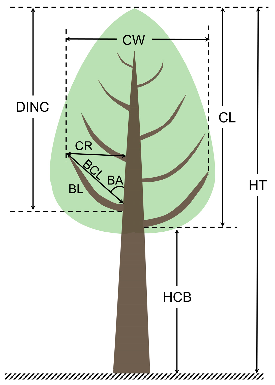
Numerous models have been developed to describe trees’ CVPs [8]. The crown radius (CR) is an essential variable for developing CVP models; however, the challenge of accurately obtaining CR information remains unresolved. In the past, it was frequently necessary to destructively harvest trees first, and then measure the branch attributes, and finally, use trigonometric relationships to compute the crown radius [9,10]. This field measurement allows the accurate acquisition of crown radius values for any height and is undoubtedly one of the most reliable and efficient methods [1]. However, field measurements can be labor- and material-intensive and time-consuming [11], and even natural forests are not allowed to be destructively harvested due to the natural forest protection policy [12] in China. Remote sensing technology has been developed to provide a new solution for detecting forest parameters with better time efficiency and cost efficiency, and it is regarded as an alternative way to solve the limitations of field surveys [13].

As an active remote sensing approach, LiDAR has emerged as a feasible tool for extracting crucial forest parameters [14] since it can penetrate the forest canopy to reach the ground and provide vertical structure and topography information [15]. Over the past two decades, LiDAR platforms have been rapidly developed, including satellite platforms (CALIOP), airborne platforms (airborne laser scanning (ALS)), and near-ground platforms (terrestrial laser scanning (TLS) and backpack laser scanning (BLS)), which provide technical support for monitoring a wide range of forest dynamics changes. LiDAR enables the capture of sensitive and detailed forest structure information, consisting of sample plot and tree level crown and trunk attribute measurements [16,17,18,19,20,21]. Furthermore, many efficient individual tree detection (ITD) [22,23,24,25,26] and individual tree crown detection (ITCD) algorithms [27,28,29,30,31,32] have been gradually developed to improve the ability to describe individual tree structures in detail and to lay the foundation for extracting CVPs.

Terrestrial laser scanning (TLS) can provide high-accuracy and high-density point cloud data, which have been used to restore the 3D structure of individual trees in detail [33]. TLS has been utilized by researchers to extract common individual tree attribute metrics, such as diameter at the breast height (DBH), tree height, and position of individual trees [34,35,36,37,38]. It also enables the description of crown attributes, such as the crown width, crown volume, crown surface area [39,40,41,42], and other crown metrics [43], which provide direct evidence to rationalize the effects caused by competition on the crown. Additionally, TLS also allows the calculation of individual tree volume [44,45] and biomass [46,47]. Recent research has demonstrated that the detailed structure of tree trunks and branches can be reconstructed using TLS data and quantitative structural models (QSM) [48,49,50,51,52,53]. As a result, QSM can be utilized to examine whole-tree topology and indirectly determine the tree wood volume and aboveground biomass [47,54]. However, surprisingly, a few studies have used TLS to develop CVP models, even though TLS can accurately characterize tree metrics.

To date, researchers have mainly used the ‘cumulative width percentile’ in layered point cloud data to determine the outer contour points of the crown point cloud, and then defined the horizontal distance from the outer contour points to the center of the trunk as the CR for developing the CVP model. For instance, Ferrarese [8] developed a regional CVP model for three conifer species in the interior of the north-western United States by using a point cloud at the 95th percentile in a point cloud height bin of increments of 0.25 m as the outer CVP points. This is the first documented report on the application of TLS to develop a CVP model. Quan [1] et al. developed a CVP model for larch in north-eastern China based on UAV-LS data. The findings of the comparison between the prediction results and those of previously published CVP models developed using field measurement data showed that there was strong agreement between them. Both research findings imply that developing tree CVP models based on point cloud data have great potential. However, none of the above studies provide the specific accuracy of extracting outer crown contour points (or crown radius) based on point clouds, and strong evidence for using point cloud data instead of actual measurement data for individual tree attribute studies is not provided.

Previously developed CVP models mainly used ordinary least squares (OLS) regression to estimate the model parameters [55,56,57,58], which ignored random errors arising from different levels due to the usual hierarchical nested structure of the modeling data, resulting in the poor prediction accuracy of the models. The mixed-effects model consists of two parts, fixed effects and random effects [59,60], which can not only estimate the average trend of the overall sample, but also reflect the differences between different ‘levels’, thus significantly improving the prediction accuracy of the model. Gao [61] developed a mixed-effects model of the plot-level CVP using field-measured branch data from 49 larch plants to explain the differences in CVPs between different sites. Zhao [62] et al. developed a two-level CVP mixed-effects model using field-measured branch data from 58 northern Chinese larch plants. The results showed that the prediction effect of the two-level CVP mixed-effects model was significantly more effective than that of the one-level mixed-effects model. However, the above researchers developed mixed-effects models for CVPs by selecting numerous sample trees from the sample plots for destructive harvesting to obtain modeling data. We have no idea whether these selected sample trees can adequately represent the growth conditions of all trees in the sample plots; therefore, the mixed-effects models they developed are limited in terms of representativeness.

Overall, due to the expensive acquisition of data, previous studies on CVP models have primarily focused on a limited number of trees, which has resulted in an inability to adequately characterize the crown at the regional level. Data from the TLS can produce a larger, more detailed sample, which makes it possible to develop regional-level CVP models. Therefore, in this paper, the main objective is to develop a CVP model using TLS at the sample plot scale to complement an individual tree-based CVP model and improve its applicability and prediction accuracy. The specific objectives are (1) to propose a method for the automatic extraction of crown radii at different heights using TLS point cloud data; (2) to develop a two-level mixed-effects model for the CVP using the extracted crown radii. This study provides an efficient method to accurately access crown information and enrich the means of conducting forest surveys. At the same time, our results can contribute theoretical support to accurately characterize crown characteristics at the regional level, which is beneficial for forest managers to develop reasonable forest management strategies.

2. Materials and Methods

2.1. Study Area

The study area is in Mengjiagang Forestry Farm, Huanan County, Jiamusi City, Heilongjiang Province, which was established in February 1956 and is one of the first state-owned forestry farms to be established in Heilongjiang Province after the founding of the People’s Republic of China, subordinate to the Jiamusi Forestry Bureau. Moreover, the administrative area belongs to the territory of Huanan County. The geographical coordinates are 130°32′~130°52′E, 46°20′~46°30′N, as shown in Figure 1. The landforms are mainly low hills with gentle slopes and an average elevation of 250 m. The forestry operation covers a total area of approximately 16,000 hectares, with a total forest accumulation of 1.41 million cubic meters. The forestry operation is mainly based on planted forests, of which 2/3 of the entire operation area is planted forests, and 1/3 is natural secondary forests, with a forest coverage rate of 81.7%. The tree species are primarily conifers, including Pinus koraiensis, Picea asperata, Pinus sylvestris var. mongholica, Larix olgensis, etc.

2.2. Field Measurement Data

In September 2020, we investigated 6 planted Korean pine sample plots of 0.06 ha in size (20 m × 30 m) at the Mengjiagang forest farm. These samples had different attributes (density, age, and elevation). All individual trees with a DBH over 5 cm in the sample plots were measured. Specifically, the DBH of the tree was measured using diameter tape, the tree height and crown base height (HCB) were measured with an ultrasonic altimeter (Vertex IV, Haglöf Sweden, Sweden), and the crown width (CW) of the tree in different directions was measured with steel tape. In addition, we also measured the geographic coordinates of all trees in the sample plots by combining real-time kinetic (RTK) technology and a global navigation satellite system (GNSS). More detailed statistical information regarding the sample plots is shown in

Table 1. Basic overview of 6 planted Korean pine sample plots.

Plots	Density (N·hm−2)	Age (Year)	Elevational (m)	Mean Height (m)	Mean DBH (cm)	Mean CW (m)	Mean HCB (m)
1	800	47	237	13.3	21.5	4.4	6.0
2	567	57	260	15.4	25.2	4.7	5.9
3	500	47	245	14.4	26.8	5.6	4.5
4	700	45	263	13.8	23.1	4.6	5.8
5	850	49	260	14.2	23.0	4.5	6.9
6	1033	42	221	13.8	19.6	4.1	8.3

.

The sample trees were selected with the following method. Each plot’s trees were arranged according to their DBH in ascending order. The cumulative percentage of the basal area was then divided into five even intervals, each representing 20% of the plot basal area, after the cumulative basal area had been calculated and divided by the plot basal area. Finally, the average diameter of the trees in each interval was calculated, and the tree with a value closest to the average diameter was selected as the sampling tree. A total of 30 sample trees were selected to destructively measure the branch attributes. We took care to cut down sample trees and tried to keep the crown undamaged. After felling, the tree height and HCB were measured using a tape measure, and the distance from the HCB to the tree top was the crown length (CL). Then, the whole tree was cut into 1 m sections at the beginning of the stump, and the sections were numbered. When measuring the branching factor, stem sections were placed vertically on the ground to maintain the branches in their most natural growth state and group all the branches with a vertical spacing of less than 20 cm into the same whorl. The following branching factors (Figure 2) were measured: the branch length (BL), which is the length measured tightly against the branch; the branch chord length (BCL), which is the straight line distance between the start and end of the branch; the branch angle (BA), which is the angle between the chord length and the trunk of the tree; the branch depth into the crown (DINC). Additional crown parameters were also calculated: the crown radius (CR), CR = BCL × sin (BA) and the relative depth into the crown (RDINC), RDINC = (DINC – BCL × cos (BA))/CL. A total of 2581 branches were measured from 30 sample trees. We selected the largest branch (this branch has the largest CR) in each whorl of all sample trees, 616 in total, and used them as reference data to validate the extraction of the CR using point cloud data. Descriptive statistics of the sample trees and branches are shown in

Table 2. Descriptive statistics of tree factors and branch factors from destructively harvested sampled trees.

Statistics	Tree Factors (N = 30)				Branch Factors (N = 616)
	Height (m)	DBH (cm)	CW (m)	HCB (m)	BL (cm)	BC (cm)	VA (°)
Max	16.1	33.0	7.9	10.0	628	607	110
Min	12.3	12.9	1.7	4.3	9	6	5
Mean	14.4	22.5	4.9	7.8	152	139	54
Std	0.91	5.26	1.57	1.49	98	92	13

.

2.3. TLS Data

On a clear and windless day, we collected point cloud data from 6 sample plots and 30 sample trees via Trimble TX8 (Trimble, CA, USA) terrestrial laser scanning (

Table A1. Information about scanning devices.

Parameters	Trimble TX8
Weight (kg)	10.7
Ranging accuracy (mm)	±2
Point spacing at 30 m (mm)	5.7
Field of view	360° × 317°
Angle measurement accuracy (μrad)	80

). Regarding the sample plots, we scanned sample plots from five positions (Figure 3 right) to ensure the integrity of the point clouds of the sample trees within the plots and to avoid missing point clouds due to mutual occlusion between the sample trees [63]. Specifically, a scanning station was placed in the center of the sample plot, and the scanning time was set to 10 min. Four corners of the sample plot were each placed in a scanning station, and the scanning time was set to 3 min. Notably, when the scanning stations is placed at the sample plot corner points, the TLS should be placed at a distance of 5 m outside the sample plot corner points to ensure the integrity of the sample trees near the sample plot corner points. Regarding the purpose of the co-registration of multi-station cloud data, 10 reflection target balls (RETB) were placed evenly around the sample plot, with the height of the RETB was staggered as much as possible to avoid mutual blockage between the RETB and to ensure that at least three or more RETB at the same time can be observed at each scanning site. The average time spent collecting TLS data for each sample plot was 45 min.

For sample trees, we scanned sample trees from three positions (Figure 3 left) to ensure that the point cloud could cover the whole tree completely, but not cause redundancy in the data [53]. The scanning stations were evenly distributed around the perimeter of the sample tree at an angle of 120° as far away as possible, and the distance between each scanning station and the sample tree was approximately the size of the tree’s height. Five RETBs were evenly placed within 2 m of the sample trees, and at least two RETBs could be observed at each scanning station to allow later co-registration of the point cloud data. Weeds and low bushes that may cause shading around the sample trees were removed before scanning began, and the scanning time was set to 10 min for each scanning station.

2.4. Pre-Processing the Point Cloud Data

The co-registration of multi-station point cloud data was implemented using Trimble RealWorks 11.2 software (Trimble, CA, USA), which accompanied Trimble TX8. A single-point matching method was used for co-registration using RETB as the reference target. When the error was less than 5 mm after refinement during the matching process, it was considered to be successful. To solve the problem of data redundancy, we used ‘Octree’ to downsample the point cloud data [64,65]. An improved progressive triangulated irregular network densification (IPTD) filtering algorithm [66,67] was used to separate ground points from non-ground points. The digital elevation model (DEM) was then generated via irregular triangular mesh interpolation to facilitate the normalization of the point cloud. TLS works via a bottom-up scanning method that clearly identifies the stem; therefore, we apply a bottom-up approach for individual tree segmentation. The trunk was first detected using a clustering algorithm, and then the shortest path algorithm based on metabolic ecology theory was used to segment the crown [68] for the purpose of segmenting the complete individual tree. The individual tree segmentation step was performed using Lidar360 software (Beijing Digital Green Soil Technology Co., Ltd., Beijing, China), and the segmentation results contain DBH, CW and tree height information, as well as the coordinate positions of the individual trees. Figure 4 summarizes the workflow of this study.

2.5. The Procedure of the Crown Radius Extraction Automatically

2.5.1. Automatic Detection of the HCB

The crown base height (HCB) is generally defined as the vertical distance from the ground at the base of a continuous living crown [69,70,71,72], and the precision of the HCB determines the integrity of the crown. In this study, the principle of automatic HCB detection is based on variation in the point cloud frequency distribution over the vertical profile of individual trees [1,11,73]. When the point cloud frequency increases dramatically along the tree height direction for the first time and is above a certain threshold, we determine this position as the HCB (Figure 5). To obtain details, first, the individual tree point clouds were sliced from bottom to top at a thickness of 0.1 m, and then the number of point clouds within each slice was counted to calculate the percentage of the number of point clouds within each slice to the total number of point clouds in the individual tree. Afterward, the vertical distribution of the point cloud frequency was smoothed using Gaussian regression, followed by the calculation of the local maximum and minimum values. The HCB is defined as the local minimum before the first local maximum above the mean point cloud frequency. To verify the effectiveness of automatic HCB detection, we calculated the detection accuracy of the HCB with the field-measured HCB as the reference value.

2.5.2. Automatic Detection of the Tree Trunks

Regarding field measurements, the horizontal distance from the branch tip to the trunk surface is commonly regarded as the CR at a certain crown level. It is essential to detect trunk points from the tree crown point cloud data to more accurately compare and analyze the differences between the CR extracted using point cloud data and the actual CR measured in the field. In this study, we applied the random sample consensus (RANSAC) algorithm [74,75] for the detection of trunk point clouds in a 2D projection plane. RANSAC is an iterative algorithm that correctly estimates the mathematical model parameters from a set that contains “outliers” [76]. A basic assumption for the RANSAC algorithm is that the data are composed of “inliers” and “outliers”. The “inliers” are data that contribute to the model parameters, and the “outliers” are data that do not fit the model.

A tree trunk’s projection plane is generally considered to be circular or elliptical. These shapes can be perfectly adapted to the detection of trunk point clouds by iteratively fitting circles using the RANSAC algorithm. In this study, the trunk point cloud was sliced with a thickness of 50 cm to avoid projection plane distortion caused by excessive trunk tilt, and then RANSAC was applied to detect the trunk point cloud in the two-dimensional projection of the sliced point cloud. RANSAC is, by nature, an iterative algorithm [77,78]. Thus, detecting the trunk point cloud from the sliced crown point cloud requires a large amount of calculations and may cause the fit to fail since the crown point density (‘outlier’) is much greater than the trunk point density is (‘inliers’). Therefore, to improve the operation efficiency and success rate of the algorithm, we continued to refine the sliced point clouds to ensure that the trunk point clouds were dominant in the refined sliced point clouds. Specifically, we use a 50 cm thick point cloud slice below the HCB height as the initial slice from which the initial circle center and diameter were detected. When we were detecting a new slice, we constructed a buffer (Figure 6) with the fitted circle center and diameter from the previous slice as the new circle center and search radius, respectively, to refine the point cloud in the new slice.

2.5.3. Automatic Detection of the Crown Outer Contour Points

The CVP model is a function of the CR at any height as the dependent variable and the distance from the CR to the treetop as the independent variable, and it is a curvilinear equation used to model the pattern of vertical variation in the shape of the tree crown [1]. Therefore, it is essential to obtain the CR at different heights to simulate the CVP. In this study, we separated the crown point cloud (Figure 7a) from the individual tree point cloud according to the HCB in Section 2.5.1, and then used the point cloud sliced projection method for the extraction of the crown radius using MATLAB R2020b (MathWorks, Natick, MA, USA) software. With reference to Gao [61] and Quan [1] et al., we chose 0.5 m as the slice thickness (Figure 7b). The convex hull algorithm [79] is a common algorithm used for finding the outermost points from a scattered set of points, and many studies have been conducted and used this algorithm for the extraction of tree crown attributes [80,81,82,83,84]. We use the 2D convex hull algorithm to find the outer contour point from the crown point cloud after projection (Figure 7c) and subsequently define the difference between the distance from the outer contour point to the trunk centroid and the trunk radius of that layer as the CR. The trunk detection method is described in Section 2.5.2.

TLS takes a bottom-up scanning approach; so, some ‘noise’ will inevitably appear in the upper part of the tree crown, resulting in an abnormally extracted CR. In this study, we applied the ‘boxplot method’ [85] to remove outliers from the extracted CR. After removing the outliers from the CR, the largest radius was selected as the maximum CR for that layer. The principle of the ‘boxplot method’ to detect outliers is to label the points above the upper limit and below the lower limit as outliers (Figure 8). The formulas for calculating the upper and lower limits are as follows:

$$upper limit=Q3+1.5\times IQR$$

(1)

$$lower limit=Q1-1.5\times IQR$$

(2)

$$IQR=Q3-Q1$$

(3)

where $Q3$ is the third quartile, which is also known as the “upper quartile” and is equal to the 75th percentile of all values in the sample ordered in ascending order; $Q1$ is the first quartile, which is also known as the “lower quartile” and is equal to the 25th percentile of all values in the sample ordered in ascending order; $IQR$ is the interquartile range.

2.5.4. Accuracy Analysis of the Extracted CR

To reduce the influence of the trees’ height on the extraction accuracy, the maximum CR extraction accuracy was analyzed in this study in the RDINC range [86]. RDINC ranges were grouped at 0.05 intervals, and then the radius values calculated from the largest branches of each whorl in 30 sampled trees served as reference values to compare and analyze the maximum CR actually measured in each RDINC range and the maximum CR extracted from the point cloud data. If the largest branches of two whorls are too close to each other in the actually measured data of the sampled trees, the maximum CR values calculated from these two branches will fall into the same RDINC range, and only the largest CR of the two will be compared in this case. If the maximum branches of two whorls are too far apart, some RDINC ranges will have no actually measured radius values. Therefore, not all extracted CRs have actually measured values for comparison. In this study, only those parts of the actually measured and extracted values that correspond to each other were compared. The evaluation indexes of the extraction accuracy are as follows:

$$P=\left(1-\frac{1}{n}{{\displaystyle \sum }}_{i=1}^n\frac{\left|X_i-x_i\right|}{X_i}\right)\times 100\%$$

(4)

$$Bias={{\displaystyle \sum }}_{i=1}^n\frac{X_i-x_i}{n}$$

(5)

where $P$ is the extraction accuracy, $n$ is the number of samples, $X_i$ is the extracted $CR$, and $x_i$ is the field-measured $CR$.

2.6. Development of the Crown Vertical Profile Model

The Weibull function is a popular function used in forest modeling [87,88]. Ferrarese [8] and Gao [89] et al. have modified the Weibull function in order to make it more applicable to the trend of CVP variation in different tree species, respectively. In this study, a modified 3-parameter Weibull function was applied to model the Korean pine CVP. The formula for the 3-parameter Weibull function is as follows:

$$CR=c·\left(\frac{b}{a}\right)·{\left(\frac{RDINC}{a}\right)}^{b-1}·e^{-{\left(\frac{RDINC}{a}\right)}^b}$$

(6)

where $CR$ is the crown radius, $a$, $b$, and $c$ are the model parameters, and $RDINC$ is the relative depth into the crown.

The shape of the CVP varies for different sizes of trees and has been reparametrized to improve the generalizability of the model [89]. We fitted the parameters of Model (6) with the measured data of the 616 largest branches of 30 sampled trees, and then analyzed the correlation between each parameter and the individual tree factors (DBH, H, CL, HD, and CW). Finally, the factors with a high level of correlation were introduced into Model (6). The formulation of the reparametrized model is as follows:

$$CR=\left(c_1+c_2·CW+c_3·DBH\right)·\left(\frac{b_1+b_2·CL}{a_1+a_2·CW}\right)·{\left(\frac{RDINC}{a_1+a_2·CW}\right)}^{\left(b_1+b_2·CL\right)-1}·e^{-{\left(\frac{RDINC}{a_1+a_2·CW}\right)}^{\left(b_1+b_2·CL\right)}}$$

(7)

where $CR$ is the crown radius; $a_1$, $a_2$, $b_1$, $b_2$, $c_{1 }$, $c_2$, and $c_3$ are the model parameters; $RDINC$ is the relative depth into the crown; the $DBH$ is the diameter at the breast height; the $CW$ is the crown width; the $CL$ is the crown length.

The data used for the development of forest growth models often have a hierarchically nested structure [90], such as individual tree data nested within sample plot data. Therefore, the ordinary least squares regression model developed can only reflect the overall average and cannot explain the differences between individuals due to some differences in the study subjects over time or space [91]. In this context, we developed a two-level (plot-level and nested tree level) mixed-effects model [59] to account for the random disturbance to the CVP of individual trees within different plots. In addition, we also developed one-level (plot level and tree level) mixed-effects models to illustrate the differences in the effects of sample plot conditions and tree size on the CVP via comparative analysis, respectively. The mixed-effects model was formulated as follows:

$$Y_{ijk}=A_{ijk}\chi +B_{i,jk}{\beta }_i+C_{ijk}{\beta }_{ij}+{\epsilon }_{ijk},i=1,···,M,j=1,···,M_i,k=1,···n_{ij}$$

(8)

where $i$, $j$, and $k$ are the plot level, the tree level within the plot level, and the observation of the crown radius, respectively; $M$ is the number of sample plots; $M_i$ is the number of sample trees within the $i$th sample plot; $n_{ij}$ is the number of crown radii on the $j$th tree within the $i$th sample plot; $Y_{ijk}$ is the observed value of the $k$th crown radius on the $j$th tree within the $i$th sample plot; $A_{ijk}$, $B_{i,jk}$, and $C_{ijk}$ are known as the design matrices; $\chi$ is the fixed effect vector; ${\beta }_i$ is the sample plot level random effect vector; ${\beta }_{ij}$ is the sample tree level random effect vector; ${\epsilon }_{ijk}$ is the error term.

2.7. Model Evaluation and Validation

In this study, we performed the random sampling of all data, with 75% of the data being used to fit the model, and the remaining 25% being used to validate the prediction of the model. $R_a^2$ and RMSE were applied to evaluate the fitting effect of the model. The larger $R_a^2$ is and the smaller RMSE is, the better the fitting effect of the model is. MAE and RMAE were applied to validate the prediction effect of the model; the smaller MAE and RMAE are, the better the prediction effect of the model is. The formula for each evaluation index is as follows:

$$R_a^2=1-\left[\frac{{\sum }_{i=1}^n{\left(y_i-{\widehat{y}}_i\right)}^2}{{\sum }_{i=1}^n{\left(y_i-{\overline{y}}_i\right)}^2}\right]·\left(\frac{n-1}{n-p}\right)$$

(9)

$$RMSE=\sqrt{\frac{{\sum }_{i=1}^n{\left(y_i-{\widehat{y}}_i\right)}^2}{n-p}}$$

(10)

$$RMAE=\frac{1}{n}{\displaystyle \sum }_{i=1}^n\left|\frac{y_i-{\widehat{y}}_i}{y_i}\right|\times 100\%$$

(11)

$$MAE={\displaystyle \sum }_{i=1}^n\left|\frac{y_i-{\widehat{y}}_i}{n}\right|$$

(12)

where $y_i$ is the observed value, ${\widehat{y}}_i$ is the predicted value, n is the number of samples, $p$ is the number of model parameters, and ${\overline{y}}_i$ is the average of all the observed values.

Regarding the mixed-effects model, the fixed-effects component was validated in the same way as for the OLS model, with an emphasis on the prediction of random parameters. We applied a quadratic sampling method to calculate random parameter values and used the empirical best linear unbiased predictor (EBLUP) [92] to calculate random effects in the model validation according to the following formula.

$$\begin{array}{c}{\widehat{\beta }}_k=\widehat{D}{\widehat{Z}}_k^T{\left({\widehat{Z}}_k\widehat{D}{\widehat{Z}}_k^T+{\widehat{R}}_k\right)}^{-1}{\widehat{\epsilon }}_k\end{array}$$

(13)

where ${\widehat{\beta }}_k$ is the random effect parameter; $\widehat{D}$ is the variance-covariance matrix of the random effect parameter; ${\widehat{Z}}_k$ is the design matrix; ${\widehat{R}}_k$ is the within-group variance-covariance matrix; and ${\widehat{\epsilon }}_k$ is the difference between the observed and predicted values calculated based on the fixed-effect parameter. Then, the results were evaluated using corresponding statistical indicators.

3. Results

3.1. HCB Extraction Results

We extracted the HCBs from a total of 283 trees from six sample plots, and Figure 9 shows the results of the extracted HCBs compared with the field-measured HCBs. In general, there was excellent correlation between the TLS-based extracted HCBs and the field measurements, with an R² of 0.905 and an RMSE of 0.52 m. All the scatter points are mainly concentrated in the lower part of the 1:1 reference line, which proves that the extracted HCBs are generally lower than the HCBs measured in the field are.

Table 3. Descriptive statistics of TLS-based extracted HCB and field-measured HCB in 6 sample plots.

Plots	Field Measurement (m)				Extraction (m)				P (%)	Bias (m)
	Max	Min	Mean	Std	Max	Min	Mean	Std
1	8.8	2.9	5.95	1.23	8.6	3.1	5.87	1.16	94.6	−0.17
2	7.3	3.3	5.91	1.18	7.1	3.7	5.77	0.97	94.5	−0.19
3	7.7	2.4	4.52	1.14	6.9	2.9	4.26	0.94	94.2	−0.21
4	8.0	4.0	5.78	0.86	7.9	4.2	5.69	0.81	94.2	−0.17
5	9.2	5.0	6.90	0.89	8.9	5.2	6.61	0.88	94.4	−0.22
6	11.2	5.7	8.28	1.11	10.5	5.7	8.09	0.95	95.4	−0.20

shows the statistical information from the HCB extraction results from different plots, and the results demonstrate that there is minimal difference in the extraction accuracies between different plots, with P being higher than 94.4%, and the biases all being negative. These results prove that the HCBs are underestimated in all plots.

3.2. CR Extraction Results

In this study, we extracted a total of 392 CRs from the point cloud data of 30 sampled trees and 3757 CRs from the point cloud data of 283 individual trees from six sample plots. The analysis of the extraction accuracy was then carried out using the branch factor data measured in the field from 30 sampled trees as reference values. The results of the extracted CRs based on point cloud data are shown in

Table 4. The results of CRs extraction from 283 trees in 6 sample plots.

Factors	Modeling Datasets					Validation Datasets
	Number	Max	Min	Mean	Std	Number	Max	Min	Mean	Std
H (m)	212	17	11.3	14.1	0.91	71	16.8	12.2	14.3	1.01
CW (m)	212	7.5	2.4	4.8	0.96	71	7.3	2.4	4.9	1.04
DBH (m)	212	33.9	14	22.6	4.02	71	35	14.7	23.3	4.71
HCB (m)	212	9.6	2	6.4	1.38	71	8.3	3.5	6.2	1.21
CR (m)	2813	3.54	0.05	2	0.78	944	3.52	0.05	2	0.81

, where we applied a random sampling method to group the data into modeling and validation datasets at a 3:1 ratio.

3.2.1. Removal of Outliers of CRs

We evaluated the differences between the directly extracted CRs (Method 1) and the field-measured CRs and the differences between the extracted CRs after removing outliers (Method 2) and the field-measured CRs, respectively. The detailed results are reflected in Figure 10. Overall, the trend of the CRs extracted via the two methods is consistent with the trend of the CVP shape along the RDINC. The differences were mainly in an RDINC range from 0 to 0.3 (Figure 10c). More specifically, in the RDINC range of 0~0.03, the directly extracted CRs are greater than those of the field measurement (Figure 10a), while the extracted CRs after the outliers were removed are already very similar to the field measurements (Figure 10b). In the end, we took the extracted CRs after removing the outliers as the result.

3.2.2. Extraction Accuracy of CRs

Table 5. Summary of CR extraction accuracy from 30 sampled trees obtained via TLS.

Range of RDINC	Number of Matching Groups	Extraction Accuracy (%)	Bias (m)
0–0.05	21	73.24	0.1121
0.05–0.1	20	78.88	0.1316
0.1–0.15	17	79.97	0.1296
0.15–0.2	17	90.23	0.1445
0.2–0.25	15	90.06	0.0947
0.25–0.3	15	90.81	0.1275
0.3–0.35	15	90.73	0.1976
0.35–0.4	15	90.39	0.1563
0.4–0.45	17	92.30	0.1138
0.45–0.5	16	94.35	0.0676
0.5–0.55	18	94.42	0.1298
0.55–0.6	18	94.81	0.1007
0.6–0.65	18	94.97	0.0668
0.65–0.7	14	93.01	0.2219
0.7–0.75	17	93.98	0.0229
0.75–0.8	15	92.33	0.2294
0.8–0.85	15	93.92	0.1095
0.85–0.9	15	91.19	0.2285
0.9–0.95	14	92.35	0.0660
0.95–1	15	90.51	0.0735
Total	327	90.12	0.1262

summarizes the CR extraction accuracy based on 30 sampled trees, and 327 sets of data were compared. It can be concluded from Table 5 that the average extraction accuracy of the CRs is 90.12%. There are variations in the extraction accuracy of CRs in different RDINC ranges. The best RDINC range is 0.15–1, and the extraction accuracies of CRs in this range are all stable at approximately 90%; the worst range is 0–0.15, with the extraction accuracies of CRs in this range all being lower than 80%. The lowest extraction accuracy of CRs is only 73.24% in the range of 0–0.05.

Figure 11 illustrates the relationship between the extracted CRs and the field-measured CRs. As shown in the figure, the scatter points are more concentrated near the 1:1 reference line, which proves that there is a strong correlation between the CRs extracted from the point cloud data and the field-measured CRs. An additional fact is that, overall, all the scatter points are mainly distributed in the upper part of the 1:1 reference line, which proves that the extracted CRs from the point cloud data led to an overestimation of the CRs.

3.3. Mixed-Effects Model

Mixed-effects model parameters were solved using the ‘nlme’ package in R software. We used all combinations of random effect parameters (128 in total), and the model failed to converge when the number of random effect parameters was greater than three.

Table 6. Fitting results of mixed-effects models with different combinations of random effects parameters.

Random Effect	Model	Random Effects Parameters	Number of Parameters	AIC	BIC	Log Likelihood	LRT	p
Base		none	7	2065.155	2112.689	−1024.580
Plot level	1	a1	8	1981.420	2034.895	−981.710
	2	c1, c3	10	1953.405	2020.887	−965.703	32.014	<0.0001
	3	c1, c2, c3	13	1937.704	2018.763	−954.852	21.700	<0.0001
Tree level	1	c2	8	1556.909	1610.383	−769.454
	2	b1, c2	10	1395.791	1461.150	−686.896	165.117	<0.0001
	3	b1, b2, c1	13	1404.556	1487.739	−688.278	2.760	0.421
Two level	1	c2	9	1550.249	1609.665	−765.124
	2	b1, c2	13	1393.398	1476.582	−682.699	164.851	<0.0001
	3	a2, b1, c2	19	1360.870	1479.703	−660.435	44.528	<0.0001

reports the evaluation of the optimal model when different combinations of the number of random effect parameters were used. Based on the AIC minimum principle [90], we selected the optimal combination of parameters for each mixed-effects model. At the plot level, the model fit performed best when the random effects were applied to parameters, c1, c2, and c3. At the tree level, the model fit performed best when random effects were applied to parameters, b1 and c2. The model fit performed best when random effects were applied to parameters, a2, b1, and c2 considering both the plot and tree levels. In addition, the LRT test results demonstrated a significant difference between the base model and the mixed-effects model (p < 0.001).

Table 7. Parameter estimates and fit statistics of the optimal model.

Model	Item	a1	a2	b1	b2	c1	c2	c3	Ra 2	RMSE (m)
Base model	Estimates	0.8074 ***	0.0503 ***	2.1119 ***	0.0348 ***	0.4545 **	0.5186 ***	0.0173 ***	0.806	0.348
		(0.0380)	(0.0079)	(0.0384)	(0.0043)	(0.1447)	(0.0334)	(0.0037)
Plot level	Estimates	0.7828 ***	0.0537 ***	2.1309 ***	−0.0360 ***	0.8071 **	0.4737 ***	0.0123 **	0.820	0.334
		(0.0380)	(0.0108)	(0.0385)	(0.0060)	(0.3512)	(0.0856)	(0.0037)
	Variance components	${\mathsf{\sigma }}^2$ = 0.3371 ${\mathsf{\sigma }}_{{\mathrm{c}}_1}^2$ = 0.5143 ${\mathsf{\sigma }}_{{\mathrm{c}}_2}^2$ = 0.0091 ${\mathsf{\sigma }}_{{\mathrm{c}}_3}^2$ = 0.0004
Tree level	Estimates	0.9226 ***	0.0188 **	2.111 ***	−0.0303 ***	0.8300 ***	0.3998 ***	0.0193 **	0.893	0.259
		(0.0408)	(0.0081)	(0.0527)	(0.0065)	(0.1740)	(0.0400)	(0.0076)
	Variance components	${\mathsf{\sigma }}^2$ = 0.2753 ${\mathsf{\sigma }}_{{\mathrm{b}}_1}^2$ = 0.0128 ${\mathsf{\sigma }}_{{\mathrm{c}}_2}^2$ = 0.0037
Two level	Estimates	0.8392 ***	0.0329 ***	2.1960 ***	−0.0377 ***	0.7598 ***	0.4288 ***	0.0136 **	0.901	0.248
		(0.0453)	(0.0105)	(0.0609)	(0.0069)	(0.1890)	(0.0448)	(0.0075)
	Variance components	${\mathsf{\sigma }}^2$ = 0.2673 ${\mathsf{\sigma }}_{{\mathrm{a}}_2}^2$ = 0.0001 ${\mathsf{\sigma }}_{{\mathrm{b}}_1}^2$ = 0.0037 ${\mathsf{\sigma }}_{{\mathrm{c}}_2}^2$ = 0.0016 ${\mathsf{\sigma }}_{{\mathrm{a}}_{2\mathrm{i},\mathrm{j}}}^2$ = 0.0002 ${\mathsf{\sigma }}_{{\mathrm{b}}_{1\mathrm{i},\mathrm{j}}}^2$ = 0.0196 ${\mathsf{\sigma }}_{{\mathrm{c}}_{2\mathrm{i},\mathrm{j}}}^2$ = 0.0073

Note: * represents the significance level, ‘***’ < 0.0001, ‘**’ < 0.01. The numbers in parentheses are the standard deviations of the parameter estimates.

shows the parameter estimators and fit statistics of the optimal model. The parameter estimators of all models passed the significance test. It was observed from the results of the fitted statistics that the R_a² of the model was significantly improved and the RMSE was significantly reduced after the introduction of random effects, which proves that the mixed-effects model significantly improves the model fitting effect. As shown by the comparison results of considering only the plot effect, tree effect, and both the plot and tree effects, the fitting effect of both the tree effect and two-level mixed effect is significantly better than that of the plot effect. In addition, the fitting effect of the two-level mixed effect is also improved compared with that of the tree effect.

3.4. Model Validation

In this study, we visualize the residual results of the base model and the mixed-effects model, and the results are shown in Figure 12. It is clear from the results that the residual distribution range of the base model is significantly larger than that of the mixed-effects models, proving that the model’s predictive power is significantly improved by introducing random effects. In addition, it is worth noting that the two-level mixed-effects model performs better than the one-level (plot-level or tree-level) mixed-effects model does, with a more concentrated distribution of residuals. Considering plot-level or tree-level random effects alone can improve the predictive power of the model, but only a combination of plot- and tree-level random effects can maximize the performance of the model.

Table 8. Validation results of the optimal model.

Model	Ra2	RMSE (m)	MAE (m)	RMAE (%)
Base	0.7811	0.3755	0.3002	27.532
Plot level	0.8034	0.3529	0.2817	27.017
Tree level	0.8552	0.3013	0.2424	24.505
Two level	0.8889	0.2874	0.2267	22.199

shows the results of verifying the predictive power of the base model and the mixed-effects model using independent validation datasets. It can be observed from the table that the two-level mixed-effects model has the best predictive power. The Each model was ranked as follows according to their predictive power: two-level mixed-effects model > tree-level mixed-effects model > plot-level mixed-effects model > base model. The two-level mixed-effects model increased the R_a² by 3.94%, 10.64%, and 13.8%, reduced the RMSE by 4.61%, 18.56%, and 23.46%, reduced the MAE by 6.48%, 19.52%, and 24.48%, and reduced the RMAE by 9.41%, 17.83%, and 19.37%, respectively, compared to those of the other three models.

4. Discussion

In the traditional approach, destructive harvesting is often required to obtain branch factors to simulate trends in the shape of the CVP [9,57,58,61,89]. TLS, as an active remote sensing technique, can truly and effectively restore the 3D structure of individual trees using massive point cloud data [33,48,73,93], which provides a new perspective for describing the trees’ CVP. In this study, we propose a method to automatically extract crown radii at different heights based on TLS point cloud data. The validity of the method was then verified using field measurement data from destructive harvesting. Finally, we developed a two-level nonlinear mixed-effects model for simulating the changing trend of planted Korean pine CVPs using the CRs extracted from point cloud data.

The focus of the study in this paper is on the crown portion of the tree; so, it is essential to accurately determine the HCBs. Numerous studies have demonstrated the effectiveness of automatic HCB detection using ALS point cloud data at both stand and individual tree scales [11,71,72]. In contrast, the automatic detection of HCBs using TLS point cloud data has not been reported very often [94]. In this study, HCBs were automatically detected in the plantation based on TLS point cloud data, and the results of the study showed a good correlation between the detected HCBs and the field measurements (Figure 9), which is consistent with the reported results in the literature [11]; however, we produced better R² and RMSE values. This is expected because TLS is more suitable for the accurate extraction of HCB information from forest stands because of its ability to produce a higher point cloud density in the lower forest canopy compared to that of ALS [95]. The results of HCB detection in sample plots with different stand densities (Table 3) indicated that the extraction method was not affected by stand density and was highly applicable and robust. The detection of HCBs via TLS underestimated the HCBs overall, with a bias of −0.19 m. One reasonable explanation is interference from the presence of dead branches on individual trees [8]. Wang [96] and Béland [97] have conducted research and reported that geometric or radiometric intensity features can be used to distinguish between leaves and branches on coniferous and broadleaf trees. Therefore, in future studies, considering the automatic detection of HCBs using geometric [96,98] and intensity [97,99] information will greatly improve the accuracy of HCB extraction.

In previous literature that used point cloud data to study CVP models, CRs were calculated as the horizontal distance from the crown’s outermost point cloud to the vertical line where the apex of the tree is located [1]. This ignores the effect of the degree of tree tilt and results in a large error between the calculated CR values and the actual CR values. In this study, we simulated the measurement of destructive harvesting in the field [9,58,61], in which the CRs were calculated as the distance from the crown’s outermost point cloud to the trunk surface. We detected circles from the crown point cloud projection using the RANSAC algorithm and treated them as tree trunks; the RANSAC algorithm has been demonstrated to be very suitable for extracting trunk information [74,75,100]. This reduced the error caused by the large degree of tree tilt to a certain extent and, at the same time, it can be better compared with the field measurement data to analyze the accuracy of CR extraction.

The results of this paper indicate a strong correlation between the CRs extracted using TLS data and actual field measurement data (Figure 11). Although TLS overestimates CRs in general, such a bias is within acceptable limits considering the time and effort required to obtain CRs in the field. The extraction results of the maximum CR in different RDINC ranges were generally better, but there were still large differences in the extraction accuracies between the crown top and the crown bottom, where the extraction accuracy of the crown bottom was better than that of the crown top (Figure 10). Quan [101] and Xu [102] et al. used UAV-LS point cloud data to extract CRs at different heights of Larix olgensis and Cunninghamia lanceolata (Lamb.) Hook., respectively, but they did not provide specific extraction accuracies because they did not have actual field measurement data for reference. Li [86] et al. extracted the trunk diameters of Larix olgensis at different heights in the vertical direction based on TLS data, and they found that the accuracy of the trunk diameter extraction decreased sharply when the relative height exceeded 0.9. In this study, the extraction accuracy of CRs at different heights was analyzed explicitly with reference to the branch factor data measured in a field containing 30 planted Korean pine trees harvested via destructive harvesting (Table 2). The extraction accuracy was low in the RDINC range of 0–0.15, stabilized from an RDINC of 0.15, and it remained at approximately 91%, which is consistent with the findings of Li [86]. Although trunk diameter extraction was not performed in this study, it was studied in the vertical direction using point cloud data; so, it can be compared with the results of Li’s study for mutual verification. TLS applies a bottom-up scanning method [95,103], which gradually becomes less effective as the trees become taller. Due to the mutual occlusion of tree crowns, it further increases the noise of the top crown point cloud, which eventually leads to a decrease in the accuracy of the CRs extracted at the top of the tree crown. It has been demonstrated that the fusion of UAV-LS and TLS data can restore the crown structure more clearly and completely [104]. Therefore, it will be our future goal to improve the extraction accuracy of tree crown structure information by combining LiDAR data from multiple platforms in future research.

Most of the data for forest stand growth modeling have a hierarchical structure, and nonlinear mixed-effects models are an effective approach to address this problem [90,91] and have been widely used in the development of tree CVP models [61]. The subject of this paper was 283 individual trees from six sample plots with different attributes, which makes it very suitable for developing a mixed-effects model. With the aim of adequately explaining the random disturbances caused by sample plots and sample trees on the trees’ CVP, we developed tree-level, plot-level, and two-level mixed-effects models. In the process of fitting a mixed-effects model, the model can have difficulty converging as the random effects increase [105]. We have adequately considered all combinations of random effect parameters, and the results show that the model does not converge when there are more than three random effect parameters. The mixed-effects model has a significantly better fit than the base model does (Table 8), demonstrating that the introduction of random effects can greatly improve the prediction accuracy of the model, which is consistent with the research results of Gao [61] and Liu [105] et al. Ferrarese [8] et al. reported that the CVP was not strongly influenced by the tree size and sample site conditions. This is because their study samples were biased toward more open stand conditions and bare canopies. The plot-level mixed-effects model we developed reflects differences between the sample plots, such as the stand density, indicating that all sample plot factors have some effect on the CVP. The tree-level mixed-effects model outperformed the sample plot-level mixed-effects model, which indicates that the differences in the CVP models were mainly due to random disturbances caused by different size sample trees. The two-level mixed-effects model had the best performance compared to those of the plot-level mixed-effects model and the tree-level mixed-effects model, which demonstrates that considering both the plot-level and tree-level effects was more effective at adequately explaining the random influence on the tree crown outer profile model.

Roeh [106] and Cluzeau [58] chose to use an indirect method to describe the CVP, as they considered that there were many difficulties in directly measuring the crown radius at different heights. TLS can provide detailed information regarding the crown structure, which is very suitable for directly describing the CVP [8], and thus, successfully overcomes the abovementioned difficulties. The previously developed CVP models based on field measurements usually require the destructive harvesting of trees, and as a result, the study sample is very limited, e.g., (Marshall [9], 36 western hemlock; Doruska [107], 34 loblolly pine; Linnell Nemec [49], 45 amabilis fir, 60 lodgepole pine, and 60 white spruce). In this study, we automatically extracted the crown radii of different heights from 283 individual trees in six sample plots using TLS without destructive sampling. It produced a large sample size and a representative dataset. A two-level mixed-effects model for the CVP was then developed based on this dataset, which greatly improved the predictive capability of the model. Overall, the results of this paper demonstrate that TLS can replace the traditional method of measuring crown structures and improve the ability to describe the CVP.

It is worth emphasizing that our proposed method is more applicable to complete crown point clouds. The subject of this study is a planted Korean pine forest, where there is less crossover between crowns; so, the crown point cloud data we obtained are complete. Using the proposed method, the crown radius of each individual tree can be extracted more successfully, which is conducive to the development of high-precision crown vertical profile models. In more complex mixed forests, crowns are difficult to be completely segmented due to the serious crossover phenomenon between the crowns. Since the crown point cloud itself is incomplete, the extracted crown radius also does not match the reality, which will seriously affect the prediction accuracy of the developed model. Therefore, a more robust crown segmentation algorithm suitable for high-density mixed forests would improve the applicability of the proposed approach. It is also an interesting topic for our future research.

5. Conclusions

TLS has great potential for accurately measuring tree crown structures and can also be used as a measurement tool in the field. In this study, we demonstrate the feasibility of the application of TLS for the development of plot-level CVP models. We propose an approach that enables the nondestructive measurement of CRs at different heights. It enables us to acquire larger amounts of data in less time and, in addition, to repeat the acquisition of data, which introduces a way to monitor dynamic changes in forest crown structures. The experimental results regarding 30 felled trees showed that the average extraction accuracy of the method was 90.12%. The extraction accuracy of the top part of the tree is poor due to the limitation of the device itself, and future research will focus on a combined UAV and TLS to improve the extraction accuracy of the CRs of the top part of the tree.

Finally, we developed mixed-effects models based on automatically extracted crown radii from 283 individual trees in six sample plots, and the results showed that the introduction of random effects significantly improved the prediction accuracy of the models. Each model was ranked as follows according to their predictive capability: two-level mixed-effects model > tree-level mixed-effects model > plot-level mixed-effects model > base model. It was demonstrated that the tree size was the main factor influencing the shape of the CVP. However, considering both the sample plot conditions and tree size could more adequately explain the differences in the CVP. Therefore, it is essential to develop CVP models on a regional scale.

References

1. Quan, Y.; Li, M.; Zhen, Z.; Hao, Y.; Wang, B. The Feasibility of Modelling the Crown Profile of Larix Olgensis Using Unmanned Aerial Vehicle Laser Scanning Data. Sensors 2020, 20, 5555. [Google Scholar] [CrossRef] [PubMed]
2. Korhonen, L.; Vauhkonen, J.; Virolainen, A.; Hovi, A.; Korpela, I. Estimation of Tree Crown Volume from Airborne Lidar Data Using Computational Geometry. Int. J. Remote Sens. 2013, 34, 7236–7248. [Google Scholar] [CrossRef]
3. Waguchi, Y. Accuracy and Precision of Crown Profile, Volume, and Surface Area Measurements of 29-Year-Old Japanese Cypress Trees Using a Spiegel Relascope. J. For. Res. 2004, 9, 173–176. [Google Scholar] [CrossRef]
4. Lu, C.; Xu, H.; Zhang, J.; Wang, A.; Wu, H.; Bao, R.; Ou, G. A Method for Estimating Forest Aboveground Biomass at the Plot Scale Combining the Horizontal Distribution Model of Biomass and Sampling Technique. Forests 2022, 13, 1612. [Google Scholar] [CrossRef]
5. Alonso-Rego, C.; Arellano-Pérez, S.; Guerra-Hernández, J.; Molina-Valero, J.A.; Martínez-Calvo, A.; Pérez-Cruzado, C.; Castedo-Dorado, F.; González-Ferreiro, E.; Álvarez-González, J.G.; Ruiz-González, A.D. Estimating Stand and Fire-Related Surface and Canopy Fuel Variables in Pine Stands Using Low-Density Airborne and Single-Scan Terrestrial Laser Scanning Data. Remote Sens. 2021, 13, 5170. [Google Scholar] [CrossRef]
6. Rowell, E.; Loudermilk, E.L.; Seielstad, C.; O’Brien, J.J. Using Simulated 3D Surface Fuelbeds and Terrestrial Laser Scan Data to Develop Inputs to Fire Behavior Models. Can. J. Remote Sens. 2016, 42, 443–459. [Google Scholar] [CrossRef]
7. Alonso-Rego, C.; Arellano-Pérez, S.; Cabo, C.; Ordoñez, C.; Álvarez-González, J.G.; Díaz-Varela, R.A.; Ruiz-González, A.D. Estimating Fuel Loads and Structural Characteristics of Shrub Communities by Using Terrestrial Laser Scanning. Remote Sens. 2020, 12, 3704. [Google Scholar] [CrossRef]
8. Ferrarese, J.; Affleck, D.; Seielstad, C. Conifer Crown Profile Models from Terrestrial Laser Scanning. Silva Fennica 2015, 49, 1106. [Google Scholar] [CrossRef] [Green Version]
9. Marshall, D.; Johnson, G.; Hann, D. Crown Profile Equations for Stand-Grown Western Hemlock Trees in Northwestern Oregon. Can. J. For. Res. 2003, 33, 2059–2066. [Google Scholar] [CrossRef] [Green Version]
10. Hann, D.W. An Adjustable Predictor of Crown Profile for Stand-Grown Douglas-Fir Trees. For. Sci. 1999, 45, 217–225. [Google Scholar]
11. Stefanidou, A.; Gitas, I.Z.; Korhonen, L.; Stavrakoudis, D.; Georgopoulos, N. LiDAR-Based Estimates of Canopy Base Height for a Dense Uneven-Aged Structured Forest. Remote Sens. 2020, 12, 1565. [Google Scholar] [CrossRef]
12. Zhang, P.; Shao, G.; Zhao, G.; Le Master, D.C.; Parker, G.R.; Dunning, J.B.; Li, Q. China’s Forest Policy for the 21st Century. Science 2000, 288, 2135–2136. [Google Scholar] [CrossRef] [PubMed] [Green Version]
13. Ferraz, A.; Mallet, C.; Jacquemoud, S.; Gonçalves, G.R.; Tomé, M.; Soares, P.; Pereira, L.G.; Bretar, F. Canopy Density Model: A New ALS-Derived Product to Generate Multilayer Crown Cover Maps. IEEE Trans. Geosci. Remote Sens. 2015, 53, 6776–6790. [Google Scholar] [CrossRef]
14. Du, L.; Pang, Y.; Wang, Q.; Huang, C.; Bai, Y.; Chen, D.; Lu, W.; Kong, D. A LiDAR Biomass Index-Based Approach for Tree- and Plot-Level Biomass Mapping over Forest Farms Using 3D Point Clouds. Remote Sens. Environ. 2023, 290, 113543. [Google Scholar] [CrossRef]
15. Giannetti, F.; Chirici, G.; Gobakken, T.; Næsset, E.; Travaglini, D.; Puliti, S. A New Approach with DTM—Independent Metrics for Forest Growing Stock Prediction Using UAV Photogrammetric Data. Remote Sens. Environ. 2018, 213, 195–205. [Google Scholar] [CrossRef]
16. Treitz, P.; Lim, K.; Woods, M.; Pitt, D.; Nesbitt, D.; Etheridge, D. LiDAR Sampling Density for Forest Resource Inventories in Ontario, Canada. Remote Sens. 2012, 4, 830–848. [Google Scholar] [CrossRef] [Green Version]
17. Bouvier, M.; Durrieu, S.; Fournier, R.A.; Renaud, J.-P. Generalizing Predictive Models of Forest Inventory Attributes Using an Area-Based Approach with Airborne LiDAR Data. Remote Sens. Environ. 2015, 156, 322–334. [Google Scholar] [CrossRef]
18. Sumnall, M.; Peduzzi, A.; Fox, T.R.; Wynne, R.H.; Thomas, V.A. Analysis of a Lidar Voxel-Derived Vertical Profile at the Plot and Individual Tree Scales for the Estimation of Forest Canopy Layer Characteristics. Int. J. Remote Sens. 2016, 37, 2653–2681. [Google Scholar] [CrossRef]
19. Andersen, H.-E.; McGaughey, R.J.; Reutebuch, S.E. Estimating Forest Canopy Fuel Parameters Using LIDAR Data. Remote Sens. Environ. 2005, 94, 441–449. [Google Scholar] [CrossRef]
20. Sumnall, M.; Fox, T.R.; Wynne, R.H.; Thomas, V.A. Mapping the Height and Spatial Cover of Features beneath the Forest Canopy at Small-Scales Using Airborne Scanning Discrete Return Lidar. Int. Soc. Photogramm. Remote Sens. J. Photogramm. 2017, 133, 186–200. [Google Scholar] [CrossRef]
21. Nie, S.; Wang, C.; Zeng, H.; Xi, X.; Xia, S. A Revised Terrain Correction Method for Forest Canopy Height Estimation Using ICESat/GLAS Data. Int. Soc. Photogramm. Remote Sens. J. Photogramm. 2015, 108, 183–190. [Google Scholar] [CrossRef]
22. Pu, Y.; Xu, D.; Wang, H.; Li, X.; Xu, X. A New Strategy for Individual Tree Detection and Segmentation from Leaf-on and Leaf-off UAV-LiDAR Point Clouds Based on Automatic Detection of Seed Points. Remote Sens. 2023, 15, 1619. [Google Scholar] [CrossRef]
23. Lisiewicz, M.; Kamińska, A.; Kraszewski, B.; Stereńczak, K. Correcting the Results of CHM-Based Individual Tree Detection Algorithms to Improve Their Accuracy and Reliability. Remote Sens. 2022, 14, 1822. [Google Scholar] [CrossRef]
24. Hershey, J.L.; McDill, M.E.; Miller, D.A.; Holderman, B.; Michael, J.H. A Voxel-Based Individual Tree Stem Detection Method Using Airborne LiDAR in Mature Northeastern U.S. Forests. Remote Sens. 2022, 14, 806. [Google Scholar] [CrossRef]
25. Ferraz, A.; Saatchi, S.; Mallet, C.; Meyer, V. Lidar Detection of Individual Tree Size in Tropical Forests. Remote Sens. Environ. 2016, 183, 318–333. [Google Scholar] [CrossRef]
26. Wang, D.; Liang, X.; Mofack, G.I.; Martin-Ducup, O. Individual Tree Extraction from Terrestrial Laser Scanning Data via Graph Pathing. For. Ecosyst. 2021, 8, 67. [Google Scholar] [CrossRef]
27. Lei, L.; Yin, T.; Chai, G.; Li, Y.; Wang, Y.; Jia, X.; Zhang, X. A Novel Algorithm of Individual Tree Crowns Segmentation Considering Three-Dimensional Canopy Attributes Using UAV Oblique Photos. Int. J. Appl. Earth Obs. 2022, 112, 102893. [Google Scholar] [CrossRef]
28. Duncanson, L.I.; Cook, B.D.; Hurtt, G.C.; Dubayah, R.O. An Efficient, Multi-Layered Crown Delineation Algorithm for Mapping Individual Tree Structure across Multiple Ecosystems. Remote Sens. Environ. 2014, 154, 378–386. [Google Scholar] [CrossRef]
29. Yun, T.; Jiang, K.; Li, G.; Eichhorn, M.P.; Fan, J.; Liu, F.; Chen, B.; An, F.; Cao, L. Individual Tree Crown Segmentation from Airborne LiDAR Data Using a Novel Gaussian Filter and Energy Function Minimization-Based Approach. Remote Sens. Environ. 2021, 256, 112307. [Google Scholar] [CrossRef]
30. Jaskierniak, D.; Lucieer, A.; Kuczera, G.; Turner, D.; Lane, P.N.J.; Benyon, R.G.; Haydon, S. Individual Tree Detection and Crown Delineation from Unmanned Aircraft System (UAS) LiDAR in Structurally Complex Mixed Species Eucalypt Forests. Int. Soc. Photogramm. Remote Sens. J. Photogramm. 2021, 171, 171–187. [Google Scholar] [CrossRef]
31. Hastings, J.H.; Ollinger, S.V.; Ouimette, A.P.; Sanders-DeMott, R.; Palace, M.W.; Ducey, M.J.; Sullivan, F.B.; Basler, D.; Orwig, D.A. Tree Species Traits Determine the Success of LiDAR-Based Crown Mapping in a Mixed Temperate Forest. Remote Sens. 2020, 12, 309. [Google Scholar] [CrossRef] [Green Version]
32. Wu, R.; Chen, Y.; Wen, C.; Wang, C.; Li, J. Delineation of individual tree crowns for mobile laser scanning data. In Proceedings of the 2nd ISPRS International Conference on Computer Vision in Remote Sensing (CVRS 2015), SPIE, Xiamen, China, 2 March 2016; Volume 9901, pp. 48–54. [Google Scholar]
33. Calders, K.; Adams, J.; Armston, J.; Bartholomeus, H.; Bauwens, S.; Bentley, L.P.; Chave, J.; Danson, F.M.; Demol, M.; Disney, M.; et al. Terrestrial Laser Scanning in Forest Ecology: Expanding the Horizon. Remote Sens. Environ. 2020, 251, 112102. [Google Scholar] [CrossRef]
34. Xia, S.; Chen, D.; Peethambaran, J.; Wang, P.; Xu, S. Point Cloud Inversion: A Novel Approach for the Localization of Trees in Forests from TLS Data. Remote Sens. 2021, 13, 338. [Google Scholar] [CrossRef]
35. Brolly, G.; Király, G.; Lehtomäki, M.; Liang, X. Voxel-Based Automatic Tree Detection and Parameter Retrieval from Terrestrial Laser Scans for Plot-Wise Forest Inventory. Remote Sens. 2021, 13, 542. [Google Scholar] [CrossRef]
36. Heinzel, J.; Huber, M.O. Tree Stem Diameter Estimation from Volumetric TLS Image Data. Remote Sens. 2017, 9, 614. [Google Scholar] [CrossRef] [Green Version]
37. Wang, D.; Hollaus, M.; Puttonen, E.; Pfeifer, N. Fast and robust stem reconstruction in complex environments using terrestrial laser scanning. In Proceedings of the The International Archives of the Photogrammetry, Remote Sensing and Spatial Information Sciences, Würzburg, Germany, 9 June 2016; pp. 411–417. [Google Scholar]
38. Wang, D.; Kankare, V.; Puttonen, E.; Hollaus, M.; Pfeifer, N. Reconstructing Stem Cross Section Shapes from Terrestrial Laser Scanning. IEEE Geosci. Remote Sens. Lett. 2017, 14, 272–276. [Google Scholar] [CrossRef]
39. Fernández-Sarría, A.; López-Cortés, I.; Estornell, J.; Velázquez-Martí, B.; Salazar, D. Estimating Residual Biomass of Olive Tree Crops Using Terrestrial Laser Scanning. Int. J. Appl. Earth Obs. 2019, 75, 163–170. [Google Scholar] [CrossRef]
40. Pitkänen, T.P.; Bianchi, S.; Kangas, A. Quantifying the Effects of Competition on the Dimensions of Scots Pine and Norway Spruce Crowns. Int. J. Appl. Earth Obs. 2022, 112, 102941. [Google Scholar] [CrossRef]
41. Srinivasan, S.; Popescu, S.C.; Eriksson, M.; Sheridan, R.D.; Ku, N.-W. Terrestrial Laser Scanning as an Effective Tool to Retrieve Tree Level Height, Crown Width, and Stem Diameter. Remote Sens. 2015, 7, 1877–1896. [Google Scholar] [CrossRef] [Green Version]
42. Estornell, J.; Velázquez-Martí, A.; Fernández-Sarría, A.; López-Cortés, I.; Martí-Gavilá, J.; Salazar, D. Estimación de parámetros de estructura de nogales utilizando láser escáner terrestre. Revista Teledetección 2017, 67, 67–76. [Google Scholar] [CrossRef]
43. Uzquiano, S.; Barbeito, I.; San Martín, R.; Ehbrecht, M.; Seidel, D.; Bravo, F. Quantifying Crown Morphology of Mixed Pine-Oak Forests Using Terrestrial Laser Scanning. Remote Sens. 2021, 13, 4955. [Google Scholar] [CrossRef]
44. Panagiotidis, D.; Abdollahnejad, A. Reliable Estimates of Merchantable Timber Volume from Terrestrial Laser Scanning. Remote Sens. 2021, 13, 3610. [Google Scholar] [CrossRef]
45. Dassot, M.; Colin, A.; Santenoise, P.; Fournier, M.; Constant, T. Terrestrial Laser Scanning for Measuring the Solid Wood Volume, Including Branches, of Adult Standing Trees in the Forest Environment. Comput. Electron. Agric. 2012, 89, 86–93. [Google Scholar] [CrossRef]
46. Momo Takoudjou, S.; Ploton, P.; Sonké, B.; Hackenberg, J.; Griffon, S.; de Coligny, F.; Kamdem, N.G.; Libalah, M.; Mofack, G.I.; Le Moguédec, G.; et al. Using Terrestrial Laser Scanning Data to Estimate Large Tropical Trees Biomass and Calibrate Allometric Models: A Comparison with Traditional Destructive Approach. Methods Ecol. Evol. 2018, 9, 905–916. [Google Scholar] [CrossRef]
47. Calders, K.; Newnham, G.; Burt, A.; Murphy, S.; Raumonen, P.; Herold, M.; Culvenor, D.; Avitabile, V.; Disney, M.; Armston, J.; et al. Nondestructive Estimates of Above-Ground Biomass Using Terrestrial Laser Scanning. Methods Ecol. Evol. 2015, 6, 198–208. [Google Scholar] [CrossRef]
48. Fan, G.; Nan, L.; Chen, F.; Dong, Y.; Wang, Z.; Li, H.; Chen, D. A New Quantitative Approach to Tree Attributes Estimation Based on LiDAR Point Clouds. Remote Sens. 2020, 12, 1779. [Google Scholar] [CrossRef]
49. Lau Sarmiento, A.; Bentley, L.; Martius, C.; Shenkin, A.; Bartholomeus, H.; Raumonen, P.; Malhi, Y.; Jackson, T.; Herold, M. Quantifying Branch Architecture of Tropical Trees Using Terrestrial LiDAR and 3D Modelling. Trees 2018, 32, 1219–1231. [Google Scholar] [CrossRef] [Green Version]
50. Brede, B.; Calders, K.; Lau, A.; Raumonen, P.; Bartholomeus, H.M.; Herold, M.; Kooistra, L. Non-Destructive Tree Volume Estimation through Quantitative Structure Modelling: Comparing UAV Laser Scanning with Terrestrial LIDAR. Remote Sens. Environ. 2019, 233, 111355. [Google Scholar] [CrossRef]
51. Qi, Y.; Coops, N.C.; Daniels, L.D.; Butson, C.R. Comparing Tree Attributes Derived from Quantitative Structure Models Based on Drone and Mobile Laser Scanning Point Clouds across Varying Canopy Cover Conditions. Int. Soc. Photogramm. Remote Sens. J. Photogramm. 2022, 192, 49–65. [Google Scholar] [CrossRef]
52. Raumonen, P.; Casella, E.; Calders, K.; Murphy, S.; Åkerblom, M.; Kaasalainen, M. Massive-scale tree modelling from tls data. Int. Soc. Photogramm. Remote Sens. Ann. Photogramm. 2015, 189–196. [Google Scholar] [CrossRef] [Green Version]
53. Raumonen, P.; Kaasalainen, M.; Åkerblom, M.; Kaasalainen, S.; Kaartinen, H.; Vastaranta, M.; Holopainen, M.; Disney, M.; Lewis, P. Fast Automatic Precision Tree Models from Terrestrial Laser Scanner Data. Remote Sens. 2013, 5, 491–520. [Google Scholar] [CrossRef] [Green Version]
54. Gonzalez de Tanago, J.; Lau, A.; Bartholomeus, H.; Herold, M.; Avitabile, V.; Raumonen, P.; Martius, C.; Goodman, R.C.; Disney, M.; Manuri, S.; et al. Estimation of Above-Ground Biomass of Large Tropical Trees with Terrestrial LiDAR. Methods Ecol. Evol. 2018, 9, 223–234. [Google Scholar] [CrossRef] [Green Version]
55. Baldwin, V.C., Jr.; Peterson, K.D. Predicting the Crown Shape of Loblolly Pine Trees. Can. J. For. Res. 1997, 27, 102–107. [Google Scholar] [CrossRef]
56. Crecente-Campo, F.; Marshall, P.; LeMay, V.; Diéguez-Aranda, U. A Crown Profile Model for Pinus Radiata D. Don in Northwestern Spain. For. Ecol. Manag. 2009, 257, 2370–2379. [Google Scholar] [CrossRef]
57. Sun, Y.X.; Feng, J.; Chen, D.; Gao, H.L.; Zou, H.T. Developing Crown Shape Model Considering a Novel Competition Index—A Case for Korean Pine Plantation in Northeast China. Can. J. For. Res. 2022, 52, 1128–1139. [Google Scholar] [CrossRef]
58. Roeh, R.L.; Maguire, D.A. Crown Profile Models Based on Branch Attributes in Coastal Douglas-Fir. For. Ecol. Manag. 1997, 96, 77–100. [Google Scholar] [CrossRef]
59. Calegario, N.; Daniels, R.F.; Maestri, R.; Neiva, R. Modeling Dominant Height Growth Based on Nonlinear Mixed-Effects Model: A Clonal Eucalyptus Plantation Case Study. For. Ecol. Manag. 2005, 204, 11–21. [Google Scholar] [CrossRef]
60. Hall, D.B.; Bailey, R.L. Modeling and Prediction of Forest Growth Variables Based on Multilevel Nonlinear Mixed Models. For. Sci. 2001, 47, 311–321. [Google Scholar]
61. Gao, H.L.; Dong, L.H.; Li, F.R. Crown Shape Model for Larix olgensis Plantation Based on Mixed Effect. Sci. Silvae Sinicae 2017, 53, 84–93. [Google Scholar]
62. Zhao, T.T.; Wang, D.Z.; Zhang, D.Y.; Guo, L.; Huang, X.R. Crown Prediction Model of Larix principis-rupprechtii Plantation in Saihanba of Hebei Province, Northern China. Sci. Silvae Sin. 2021, 57, 108–118. [Google Scholar]
63. Wilkes, P.; Lau, A.; Disney, M.; Calders, K.; Burt, A.; Gonzalez de Tanago, J.; Bartholomeus, H.; Brede, B.; Herold, M. Data Acquisition Considerations for Terrestrial Laser Scanning of Forest Plots. Remote Sens. Environ. 2017, 196, 140–153. [Google Scholar] [CrossRef]
64. Su, Y.-T.; Bethel, J.; Hu, S. Octree-Based Segmentation for Terrestrial LiDAR Point Cloud Data in Industrial Applications. Int. Soc. Photogramm. Remote Sens. J. Photogramm. 2016, 113, 59–74. [Google Scholar] [CrossRef]
65. Wang, D.; Xu, K.; Quan, Y. Structure-Aware Subsampling of Tree Point Clouds. IEEE Geosci. Remote Sens. Lett. 2022, 19, 1–5. [Google Scholar] [CrossRef]
66. Zhao, X.; Guo, Q.; Su, Y.; Xue, B. Improved Progressive TIN Densification Filtering Algorithm for Airborne LiDAR Data in Forested Areas. Int. Soc. Photogramm. Remote Sens. J. Photogramm. 2016, 117, 79–91. [Google Scholar] [CrossRef] [Green Version]
67. Nie, S.; Wang, C.; Dong, P.; Xi, X.; Luo, S.; Qin, H. A Revised Progressive TIN Densification for Filtering Airborne LiDAR Data. Measurement 2017, 104, 70–77. [Google Scholar] [CrossRef]
68. Tao, S.; Wu, F.; Guo, Q.; Wang, Y.; Li, W.; Xue, B.; Hu, X.; Li, P.; Tian, D.; Li, C.; et al. Segmenting Tree Crowns from Terrestrial and Mobile LiDAR Data by Exploring Ecological Theories. Int. Soc. Photogramm. Remote Sens. J. Photogramm. 2015, 110, 66–76. [Google Scholar] [CrossRef] [Green Version]
69. Wu, B.; Yu, B.; Yue, W.; Shu, S.; Tan, W.; Hu, C.; Huang, Y.; Wu, J.; Liu, H. A Voxel-Based Method for Automated Identification and Morphological Parameters Estimation of Individual Street Trees from Mobile Laser Scanning Data. Remote Sens. 2013, 5, 584–611. [Google Scholar] [CrossRef] [Green Version]
70. Luo, L.; Zhai, Q.; Su, Y.; Ma, Q.; Kelly, M.; Guo, Q. Simple Method for Direct Crown Base Height Estimation of Individual Conifer Trees Using Airborne LiDAR Data. Opt. Express 2018, 26, A562–A578. [Google Scholar] [CrossRef]
71. Vandendaele, B.; Fournier, R.A.; Vepakomma, U.; Pelletier, G.; Lejeune, P.; Martin-Ducup, O. Estimation of Northern Hardwood Forest Inventory Attributes Using UAV Laser Scanning (ULS): Transferability of Laser Scanning Methods and Comparison of Automated Approaches at the Tree- and Stand-Level. Remote Sens. 2021, 13, 2796. [Google Scholar] [CrossRef]
72. Novotny, J.; Navratilova, B.; Albert, J.; Cienciala, E.; Fajmon, L.; Brovkina, O. Comparison of Spruce and Beech Tree Attributes from Field Data, Airborne and Terrestrial Laser Scanning Using Manual and Automatic Methods. Remote Sens. Appl. Soc. Environ. 2021, 23, 100574. [Google Scholar] [CrossRef]
73. Reitberger, J.; Schnörr, C.; Krzystek, P.; Stilla, U. 3D Segmentation of Single Trees Exploiting Full Waveform LIDAR Data. Int. Soc. Photogramm. Remote Sens. J. Photogramm. 2009, 64, 561–574. [Google Scholar] [CrossRef]
74. Ye, W.; Qian, C.; Tang, J.; Liu, H.; Fan, X.; Liang, X.; Zhang, H. Improved 3D Stem Mapping Method and Elliptic Hypothesis-Based DBH Estimation from Terrestrial Laser Scanning Data. Remote Sens. 2020, 12, 352. [Google Scholar] [CrossRef] [Green Version]
75. Pitkänen, T.P.; Raumonen, P.; Kangas, A. Measuring Stem Diameters with TLS in Boreal Forests by Complementary Fitting Procedure. Int. Soc. Photogramm. Remote Sens. J. Photogramm. 2019, 147, 294–306. [Google Scholar] [CrossRef]
76. Olofsson, K.; Holmgren, J.; Olsson, H. Tree Stem and Height Measurements Using Terrestrial Laser Scanning and the RANSAC Algorithm. Remote Sens. 2014, 6, 4323–4344. [Google Scholar] [CrossRef] [Green Version]
77. Fischler, M.A.; Bolles, R.C. Random sample consensus: A paradigm for model fitting with applications to image analysis and automated cartography. In Readings in Computer Vision; Fischler, M.A., Firschein, O., Eds.; Elsevier: Amsterdam, The Netherlands, 1987; pp. 726–740. [Google Scholar]
78. Jin, Z.; Tillo, T.; Zou, W.; Zhao, Y.; Li, X. Robust Plane Detection Using Depth Information from a Consumer Depth Camera. IEEE Trans. Circuits Syst. Video Technol. 2019, 29, 447–460. [Google Scholar] [CrossRef]
79. Graham, R.L. An Efficient Algorith for Determining the Convex Hull of a Finite Planar Set. Inf. Process. Lett. 1972, 1, 132–133. [Google Scholar] [CrossRef]
80. Rocha, K.D.; Silva, C.A.; Cosenza, D.N.; Mohan, M.; Klauberg, C.; Schlickmann, M.B.; Xia, J.; Leite, R.V.; de Almeida, D.R.A.; Atkins, J.W.; et al. Crown-Level Structure and Fuel Load Characterization from Airborne and Terrestrial Laser Scanning in a Longleaf Pine (Pinus palustris Mill.) Forest Ecosystem. Remote Sens. 2023, 15, 1002. [Google Scholar] [CrossRef]
81. Poorazimy, M.; Ronoud, G.; Yu, X.; Luoma, V.; Hyyppä, J.; Saarinen, N.; Kankare, V.; Vastaranta, M. Feasibility of Bi-Temporal Airborne Laser Scanning Data in Detecting Species-Specific Individual Tree Crown Growth of Boreal Forests. Remote Sens. 2022, 14, 4845. [Google Scholar] [CrossRef]
82. Fernández-Sarría, A.; Martínez, L.; Velázquez-Martí, B.; Sajdak, M.; Estornell, J.; Recio, J.A. Different Methodologies for Calculating Crown Volumes of Platanus Hispanica Trees Using Terrestrial Laser Scanner and a Comparison with Classical Dendrometric Measurements. Comput. Electron. Agric. 2013, 90, 176–185. [Google Scholar] [CrossRef]
83. Yrttimaa, T.; Luoma, V.; Saarinen, N.; Kankare, V.; Junttila, S.; Holopainen, M.; Hyyppä, J.; Vastaranta, M. Exploring Tree Growth Allometry Using Two-Date Terrestrial Laser Scanning. For. Ecol. Manag. 2022, 518, 120303. [Google Scholar] [CrossRef]
84. Zhou, L.; Li, X.; Zhang, B.; Xuan, J.; Gong, Y.; Tan, C.; Huang, H.; Du, H. Estimating 3D Green Volume and Aboveground Biomass of Urban Forest Trees by UAV-Lidar. Remote Sens. 2022, 14, 5211. [Google Scholar] [CrossRef]
85. Schwertman, N.C.; Owens, M.A.; Adnan, R. A Simple More General Boxplot Method for Identifying Outliers. Comput. Stat. Data Anal. 2004, 47, 165–174. [Google Scholar] [CrossRef]
86. Li, D.; Guo, H.; Jia, W.; Wang, F. Analysis of Taper Functions for Larix Olgensis Using Mixed Models and TLS. Forests 2021, 12, 196. [Google Scholar] [CrossRef]
87. Schreuder, H.T.; Swank, W.T. Coniferous Stands Characterized with The Weibull Distribution. Can. J. For. Res. 1974, 4, 518–523. [Google Scholar] [CrossRef]
88. Saito, S.; Sato, T.; Kominami, Y.; Nagamatsu, D.; Kuramoto, S.; Sakai, T.; Tabuchi, R.; Sakai, A. Modeling the Vertical Foliage Distribution of an Individual Castanopsis cuspidata (Thunb.) Schottky, a Dominant Broad-Leaved Tree in Japanese Warm-Temperate Forest. Trees 2004, 18, 486–491. [Google Scholar] [CrossRef]
89. Gao, H.L.; Dong, L.H.; Li, F.R. Modelling outer crown profile for planted Pinus koraiensis and Larix olgensis trees in Heilongjiang Province, China. J. Nanjing For. Univ. 2018, 42, 10–18. [Google Scholar]
90. Tian, D.; Jiang, L.; Shahzad, M.K.; He, P.; Wang, J.; Yan, Y. Climate-Sensitive Tree Height-Diameter Models for Mixed Forests in Northeastern China. Agric. For. Meteorol. 2022, 326, 109182. [Google Scholar] [CrossRef]
91. Bronisz, K.; Mehtätalo, L. Mixed-Effects Generalized Height–Diameter Model for Young Silver Birch Stands on Post-Agricultural Lands. For. Ecol. Manag. 2020, 460, 117901. [Google Scholar] [CrossRef]
92. Zu, X.F.; Ni, C.C.; Nigh, G.; Qin, X.L. Based on Mixed-Effects Model and Empirical Best Linear Unbiased Predictor to Predict Growth Profile of Dominant Height. Sci. Silvae Sin. 2015, 51, 25–33. [Google Scholar]
93. Yrttimaa, T.; Luoma, V.; Saarinen, N.; Kankare, V.; Junttila, S.; Holopainen, M.; Hyyppä, J.; Vastaranta, M. Structural Changes in Boreal Forests Can Be Quantified Using Terrestrial Laser Scanning. Remote Sens. 2020, 12, 2672. [Google Scholar] [CrossRef]
94. Schneider, R.; Calama, R.; Martin-Ducup, O. Understanding Tree-to-Tree Variations in Stone Pine (Pinus pinea L.) Cone Production Using Terrestrial Laser Scanner. Remote Sens. 2020, 12, 173. [Google Scholar] [CrossRef] [Green Version]
95. Hilker, T.; van Leeuwen, M.; Coops, N.C.; Wulder, M.A.; Newnham, G.J.; Jupp, D.L.B.; Culvenor, D.S. Comparing Canopy Metrics Derived from Terrestrial and Airborne Laser Scanning in a Douglas-Fir Dominated Forest Stand. Trees 2010, 24, 819–832. [Google Scholar] [CrossRef]
96. Wang, D.; Momo Takoudjou, S.; Casella, E. LeWoS: A Universal Leaf-Wood Classification Method to Facilitate the 3D Modelling of Large Tropical Trees Using Terrestrial LiDAR. Methods Ecol. Evol. 2020, 11, 376–389. [Google Scholar] [CrossRef]
97. Béland, M.; Widlowski, J.-L.; Fournier, R.A.; Côté, J.-F.; Verstraete, M.M. Estimating Leaf Area Distribution in Savanna Trees from Terrestrial LiDAR Measurements. Agric. For. Meteorol. 2011, 151, 1252–1266. [Google Scholar] [CrossRef]
98. Wang, D.; Brunner, J.; Ma, Z.; Lu, H.; Hollaus, M.; Pang, Y.; Pfeifer, N. Separating Tree Photosynthetic and Non-Photosynthetic Components from Point Cloud Data Using Dynamic Segment Merging. Forests 2018, 9, 252. [Google Scholar] [CrossRef] [Green Version]
99. Sun, J.; Wang, P.; Gao, Z.; Liu, Z.; Li, Y.; Gan, X.; Liu, Z. Wood–Leaf Classification of Tree Point Cloud Based on Intensity and Geometric Information. Remote Sens. 2021, 13, 4050. [Google Scholar] [CrossRef]
100. Wang, D.; Hollaus, M.; Puttonen, E.; Pfeifer, N. Automatic and Self-Adaptive Stem Reconstruction in Landslide-Affected Forests. Remote Sens. 2016, 8, 974. [Google Scholar] [CrossRef] [Green Version]
101. Quan, Y.; Li, M.; Zhen, Z.; Hao, Y. Modeling Crown Characteristic Attributes and Profile of Larix olgensis Using UAV-borne LiDAR. J. Northeast For. Univ. 2019, 47, 52–58. [Google Scholar] [CrossRef]
102. Xu, Z.Y.; Liu, H.D.; Chen, Y.F.; Chen, Q.; Li, H.Y.; Wang, J. Outer Upper Crown Profile Simulation and Visualization for Cunninghamia lanceolata Based on UAV-borne LiDAR Data. For. Res. 2021, 34, 40–48. [Google Scholar] [CrossRef]
103. Wang, F.; Sun, Y.; Jia, W.; Zhu, W.; Li, D.; Zhang, X.; Tang, Y.; Guo, H. Development of Estimation Models for Individual Tree Aboveground Biomass Based on TLS-Derived Parameters. Forests 2023, 14, 351. [Google Scholar] [CrossRef]
104. Wang, M.; Im, J.; Zhao, Y.; Zhen, Z. Multi-Platform LiDAR for Non-Destructive Individual Aboveground Biomass Estimation for Changbai Larch (Larix olgensis Henry) Using a Hierarchical Bayesian Approach. Remote Sens. 2022, 14, 4361. [Google Scholar] [CrossRef]
105. Liu, X.; Hao, Y.; Widagdo, F.R.A.; Xie, L.; Dong, L.; Li, F. Predicting Height to Crown Base of Larix Olgensis in Northeast China Using UAV-LiDAR Data and Nonlinear Mixed Effects Models. Remote Sens. 2021, 13, 1834. [Google Scholar] [CrossRef]
106. Cluzeau, C.; Goff, N.L.; Ottorini, J.-M. Development of Primary Branches and Crown Profile of Fraxinusexcelsior. Can. J. For. Res. 1994, 24, 2315–2323. [Google Scholar] [CrossRef]
107. Doruska, P.F.; Mays, J.E. Crown Profile Modeling of Loblolly Pine by Nonparametric Regression Analysi. For. Sci. 1998, 44, 445–453. [Google Scholar]
Figure 1. Location of sample plots in the study area.
Remotesensing 15 03272 g001
Figure 2. Illustration of tree factors and branch factors. CW is the crown width, CL is the crown length, DINC is the depth into the crown of the branch, HCB is the crown base height, HT is the tree height, BL is the branch length, BCL is the branch chord length, BA is the branch angle, and CR is the crown radius.
Remotesensing 15 03272 g002
Figure 3. Illustrations for collecting TLS data. The (left) image shows the process of scanning the sample tree from three positions, and the (right) image shows the process of scanning sample plots from five positions.
Remotesensing 15 03272 g003
Figure 4. Workflow diagram of this study.
Remotesensing 15 03272 g004
Figure 5. (a) is the perspective view of the sample trees’ point clouds. The color scale on the left represents the height in meters and the red box shows the field-measured HCB value. (b) is an illustration depicting the process of automatically detecting HCB. The gray points are the point cloud frequency within each slice. The green line is the smoothed point cloud frequency curve. The red and blue points represent the local minima and local maxima detected on the curve, respectively. The vertical dotted line represents the mean point cloud frequency and the horizontal black line represents the detected HCB (i.e., the local minimum before the first local maximum above the mean point cloud frequency).
Remotesensing 15 03272 g005
Figure 6. (a) is a projection of the sliced crown point cloud, where the yellow part is the buffer constructed according to the parameters of the initial circle. (b) is an illustration of the process of detecting trunk points from the buffer point cloud using RANSAC algorithm. The blue points are the detected trunk points. The purple color is the circle fitted based on the trunk points.
Remotesensing 15 03272 g006
Figure 7. The process of extracting CRs on individual crown point clouds. (a) is the 3D perspective view of the individual crown point cloud. (b) shows the projection of the crown point cloud after slicing. (c) is shows the convex hull on the projection used to calculate the CR.
Remotesensing 15 03272 g007
Figure 8. Illustration of the ‘boxplot method’ for detecting outliers.
Remotesensing 15 03272 g008
Figure 9. Comparison of TLS-based extracted HCB with field-measured HCB.
Remotesensing 15 03272 g009
Figure 10. Assessing the differences in CR extraction via different methods. ‘Reference’ is the field measurement of CR from 30 sampled trees. ‘Method 1’ was used to extract the CR directly from the TLS. ‘Method 2’ involved applying the ‘boxplot method’ to remove the outliers, and then extracting the CR from the TLS. (a) is a comparison of the reference CR with the extracted CR obtained via Method 1. (b) is a comparison of the reference CR with the extracted CR via Method 2. (c) is a comparison of the extracted CR obtained via Method 1 with the extracted CR obtained via Method 2.
Remotesensing 15 03272 g010
Figure 11. Comparison of TLS-based extracted CR with field-measured CR.
Remotesensing 15 03272 g011
Figure 12. Visualization of model residual results. (a) is the base model, (b) is the plot-level mixed-effects model, (c) is the tree-level mixed-effects model, and (d) is the two-level mixed-effects model.
Remotesensing 15 03272 g012