Multi-Featured Sea Ice Classification with SAR Image Based on Convolutional Neural Network

Abstract

Sea ice is a significant factor in influencing environmental change on Earth. Monitoring sea ice is of major importance, and one of the main objectives of this monitoring is sea ice classification. Currently, synthetic aperture radar (SAR) data are primarily used for sea ice classification, with a single polarization band or simple combinations of polarization bands being common choices. While much of the current research has focused on optimizing network structures to achieve high classification accuracy, which requires substantial training resources, we aim to extract more information from the SAR data for classification. Therefore we propose a multi-featured SAR sea ice classification method that combines polarization features calculated by polarization decomposition and spectrogram features calculated by joint time-frequency analysis (JTFA). We built a convolutional neural network (CNN) structure for learning the multi-features of sea ice, which combines spatial features and physical properties, including polarization and spectrogram features of sea ice. In this paper, we utilized ALOS PALSAR SLC data with HH, HV, VH, and VV, four types of polarization for the multi-featured sea ice classification method. We divided the sea ice into new ice (NI), first-year ice (FI), old ice (OI), deformed ice (DI), and open water (OW). Then, the accuracy calculation by confusion matrix and comparative analysis were carried out. Our experimental results demonstrate that the multi-feature method proposed in this paper can achieve high accuracy with a smaller data volume and computational effort. In the four scenes selected for validation, the overall accuracy could reach 95%, 91%, 96%, and 95%, respectively, which represents a significant improvement compared to the single-feature sea ice classification method.

1. Introduction

Sea ice is primarily distributed in the polar regions and exerts a profound impact on global climate and environmental change by affecting the exchange of energy and material between the ocean and the atmosphere and by redistributing salt within the ocean [1]. In the Arctic region, sea ice variability has significant implications for the normal Arctic shipping routes [2]. Therefore, sea ice monitoring not only contributes to scientific research on polar and global climate and environment but also has important practical implications for maritime shipping and polar expeditions. As science and technology evolve, satellite remote sensing has become a better option than traditional sea ice observational methods, such as in situ and ice station observations, for increased monitoring and the ability to monitor sea ice at high spatial and temporal resolution [3].

Satellite remote sensing can monitor sea ice in the visible, infrared, and microwave regions of the electromagnetic spectrum [4]. The visible and infrared remote sensing instruments, such as the Operational Linescan System (OLS), the Moderate Resolution Imaging Spectroradiometer (MODIS), and the Visible Infrared Imaging Radiometer Suite (VIIRS), are limited by their operating hours and cloud cover, which constrain their monitoring capability for sea ice. By contrast, electromagnetic waves in the microwave band can acquire observations during both day and night and through any weather conditions [5]. Synthetic Aperture Radar (SAR), a special type of active microwave imaging radar, benefits from advanced technology and complex data, providing more detailed information on sea ice [4]. Notable SAR satellites include NASA’s Seasat SAR, the European Space Agency’s (ESA) ERS-1, ERS-2, Sentinel-1, the Canadian Space Agency’s (CSA) RADARSAT-1, RADARSAT-2, and China’s Gaofen-3 (GF-3). Over time, SAR satellites have developed from the original L-band with single polarization to the current L-, C-, and X-band SAR with dual-polarization and quad-polarization, providing a substantial amount of data and a rich source of information for sea ice monitoring.

Sea ice classification for Synthetic Aperture Radar (SAR) data serves as the foundation for both sea ice research and operational ice services [6]. Its primary objective is to identify the main sea ice features related to ice types and surface roughness and group them into predetermined categories [7]. The sea ice categories that are commonly used in current research, and also the standard for sea ice classification, are defined by the World Meteorological Organization (WMO). According to the formation and development of sea ice, WMO classified sea ice into three main categories: (1) Ice less than 30 cm thick (including new ice (NI), young ice (YI), etc.); (2) Ice 30 cm–2 m thick, known as first-year ice (FI) (including thin first-year ice and medium first-year ice); (3) Old ice (OI) (including second-year (SY) and multi-year ice (MY)) [8].

Initial SAR sea ice classification methods were based primarily on backscatter coefficients and texture features for single polarization or simple combinations of polarization bands [9,10]. However, the backscattering coefficient of sea ice can be affected by several factors, such as small-scale surface roughness and large-scale atmospheric circulation [11]. Thus the backscattering coefficients of different sea ice types are similar under certain imaging conditions, making it difficult to distinguish between them [12]. For the textural features of sea ice, although the grey level co-occurrence matrix (GLCM) and Markov Random Field (MRF) have been widely used with good results [13,14,15], the classification accuracy is affected by scale factors such as the window size, leading to unstable performance due to issues such as scaling and rotation of images.

Compared to SAR in single-polarization mode, polarimetric SAR (PolSAR) provides additional information on the backscattering mechanisms and physical characteristics of natural surfaces, allowing for a more comprehensive observation and analysis of targets from multiple perspectives [16]. Polarimetric decomposition has become the dominant research direction in the analytical use of PolSAR information. After the concept of target decomposition was introduced [17], polarimetric decomposition can be divided into two types: decompositions of the coherent scattering matrix and eigenvector decompositions of the coherency or covariance matrix based on target scattering characteristics [18]. Polarization decomposition has also been applied to sea ice classification. Scheuchl et al. [19,20] used H-$\alpha$ polarization decomposition with the Wishart classifier for sea ice classification. Singha et al. [21] extracted the polarization features by H-A-$\alpha$ decomposition and analyzed their classification performance in different bands to ultimately achieve four classes of ice and water classification. In addition, Moen et al. [22,23] used C-band quad-polarization SAR data for sea ice classification with improved Freeman decomposition.

Several sea ice classification algorithms, including random forest [24], decision tree [25], and image segmentation [26], have demonstrated reliable results. Additionally, the support vector machine has been widely applied to both sea ice type and ice/water classification [25,27,28]. However, the continuous development of deep learning in recent years has showcased its remarkable superiority over traditional physical- or statistical-based algorithms for extracting image information [29]. Deep learning frameworks have been extensively used in remote sensing image information mining, including sea ice detection, monitoring, and classification. Convolutional neural network (CNN) is a representative of Deep Neural Networks (DNN)that exhibits excellent performance in deep feature extraction and image classification [30]. Several advanced CNN structures, such as Alexnet [31], VGGNet [32], GoogleNet [33], ResNet [34], and DensNet [35], have been proposed. In general, CNN-based classification strategies include using pretrained CNNs as feature extractors, fine-tuning pretrained CNNs, or training CNNs from scratch [36]. For instance, [37] employed CNN networks for ice/water classification with Sentinel-1 SAR data and proposed a modified VGG-16 network, and trained from scratch for sea ice classification with Sentinel-2 cloud-free optical data. Tianyu et al. [38] proposed MSI-ResNet for arctic sea ice classification with GF-3 C-band SAR data and compared them with a classical SVM classifier. Zhang et al. [39] built a Multiscale MobileNet (MSMN) based on the MobileNetV3 for sea ice classification with GF-3 dual-polarization SAR data and achieved higher accuracy than traditional CNN and ResNet18 models.

Furthermore, there is a lot of current research on the classification of SAR images using CNNs, and many novel CNN structures and training methods have been proposed [40,41,42]. The central point is that CNN is designed to automatically and adaptively learn spatial hierarchies of features primarily [43]. Most current sea ice classification studies simply use a combination of backscatter coefficients from different polarization bands. However, for polarimetric SAR complex imagery, amplitude and phase information is equally vital. Although polarization decomposition provides valuable information to understand the physics of the SAR image [44], it does not provide sufficient frequency information in the CNN structure. To address this issue, Huang et al. [45] proposed Deep SAR-Net, which extracts spatial features with the CNN framework and learns the physical properties of the objects, such as buildings, vegetation, and agriculture, by joint time-frequency analysis on complex-valued SAR images. Their proposed method shows superior performance compared with the proposed CNN models only based on intensity information.

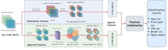
The receptive field of a CNN is crucial for the accurate detection and classification of objects in images, especially large features such as sea ice [46]. Thus current CNN-based studies on sea ice classification usually focus on the structure of neural networks, proposing many complex network models, which often require the support of a large number of samples [37,38,39]. Moreover, for the single-look complex (SLC) quad-polarization SAR data, feature extraction is insufficient in current studies on sea ice classification. In light of these limitations and inspired by existing studies, we propose a multi-featured sea ice classification method based on a convolutional neural network, where the multi-feature classification method simultaneously learns the spatial texture features of the sea ice along with backscattering information, including its physical properties. The main highlights of this paper are:

• We utilized polarization decomposition and joint time-frequency analysis to extract multi-features of the sea ice.
• We built a CNN structure that learns and fuses multi-features, including spatial texture features of sea ice and physical properties of backscatter for sea ice classification.
• The experimental results show that the multi-featured approach combines the advantages of sea ice polarization features and spectrogram features on the basis of learning the spatial features of sea ice, which improves the accuracy of sea ice classification.

2. Data Description

2.1. Data and Study Area

The Advanced Land Observing Satellite-1 (ALOS), a mission launched by the Japan Aerospace Exploration Agency (JAXA), operated from 24th January 2006 to 22nd April 2011. The Phased Array type L-band (1.27 GHz) Synthetic Aperture Radar (PALSAR) was one of three instruments on the ALOS. As an active microwave sensor using L-band frequency, PAlSAR can acquire observations during both day and night and through any weather conditions [47].

The ALOS PALSAR dataset used in this study is collected from level 1.1 product single-looked complex (SLC) SAR images of polarimetric mode (PLR) with four polarizations simultaneously (HH+HV+VV+VH), providing a spatial resolution of 30 m. The PLR mode also has an observation swath width ranging from 20 to 65 km. Previous studies have shown that the Fine Resolution model of PALSAR with an observation swath from 40 to 70 km can distinguish between deformed and level ice over all ice regimes, making it suitable for ice charting [12]. Therefore, we selected a PLR model with a similar resolution and swath width but with more polarization modes to study sea ice classification under a more diverse set of features.

This study used 30 scenes of PALSAR imagery of sea ice cover in the Arctic for experimentation.

Table 1. ALOS PALSAR SLC data used in this paper.

No.	Product	Processed Time	Incident Angle *	Usage
T1	ALOS-P1_1__A-ORBIT__ALPSRP258801420	3 December 2010	23.8998	Train
T2	ALOS-P1_1__A-ORBIT__ALPSRP180031440	11 June 2009	25.6575	Train
T3	ALOS-P1_1__A-ORBIT__ALPSRP258351550	30 November 2010	23.9199	Train
T4	ALOS-P1_1__A-ORBIT__ALPSRP258351560	30 November 2010	23.9098	Train
T5	ALOS-P1_1__A-ORBIT__ALPSRP258351570	30 November 2010	23.9004	Train
T6	ALOS-P1_1__A-ORBIT__ALPSRP226661500	26 April 2010	23.9002	Train
T7	ALOS-P1_1__A-ORBIT__ALPSRP201761520	7 November 2009	23.9201	Train
T8	ALOS-P1_1__A-ORBIT__ALPSRP233871400	15 June 2010	23.8711	Train
T9	ALOS-P1_1__A-ORBIT__ALPSRP201471450	5 November 2009	23.8996	Train
T10	ALOS-P1_1__A-ORBIT__ALPSRP257471570	24 November 2010	23.8879	Train
V1	ALOS-P1_1__A-ORBIT__ALPSRP179591440	8 June 2009	25.7066	Validation
T11	ALOS-P1_1__A-ORBIT__ALPSRP205991500	6 December 2009	23.8846	Train
V2	ALOS-P1_1__A-ORBIT__ALPSRP205991510	6 December 2009	23.8725	Validation
T12	ALOS-P1_1__A-ORBIT__ALPSRP205991520	6 December 2009	23.8613	Train
T13	ALOS-P1_1__A-ORBIT__ALPSRP065201280	16 April 2007	23.8948	Train
T14	ALOS-P1_1__A-ORBIT__ALPSRP168621400	25 March 2009	23.8619	Train
T15	ALOS-P1_1__A-ORBIT__ALPSRP200281390	28 October 2009	25.7279	Train
T16	ALOS-P1_1__A-ORBIT__ALPSRP203491180	19 November 2009	23.8325	Train
T17	ALOS-P1_1__A-ORBIT__ALPSRP274601570	21 March 2011	23.9078	Train
T18	ALOS-P1_1__A-ORBIT__ALPSRP274601590	21 March 2011	23.9201	Train
V3	ALOS-P1_1__A-ORBIT__ALPSRP279121560	21 April 2011	23.9275	Validation
V4	ALOS-P1_1__A-ORBIT__ALPSRP279121570	21 April 2011	23.9181	Validation
T19	ALOS-P1_1__A-ORBIT__ALPSRP276351580	2 April 2011	23.9046	Train
T20	ALOS-P1_1__A-ORBIT__ALPSRP276351590	2 April 2011	23.9248	Train
T21	ALOS-P1_1__A-ORBIT__ALPSRP276351600	2 April 2011	23.9165	Train
T22	ALOS-P1_1__A-ORBIT__ALPSRP277371550	9 April 2011	23.9264	Train
T23	ALOS-P1_1__A-ORBIT__ALPSRP277371560	9 April 2011	23.9165	Train
T24	ALOS-P1_1__A-ORBIT__ALPSRP062631420	29 March 2007	23.8933	Train
T25	ALOS-P1_1__A-ORBIT__ALPSRP170721430	8 April 2009	23.9053	Train
T26	ALOS-P1_1__A-ORBIT__ALPSRP179321390	6 June 2009	25.7033	Train

* The central incident angle of the images, in degrees.

provides details about the ALOS PALSAR SLC data used in this paper, including product name, imaging date, and image usage. The scenes are numbered according to their usage of the satellite data: T for training and V for validation. The spatial distribution of these scenes is shown in Figure 1.

In addition, the access dates and the central incident angles of the images are also shown in Table 1. In general, the backscatter of sea ice is known to vary with seasonal changes and incident angles, which can impact sea ice classification. However, the variation backscattering from sea ice is complex. In this study, the effect of seasonal changes is complicated by factors such as polarization and ice types. Furthermore, the incident angle mostly falls in the range of 23–27${}^{\circ }$, with a variation of $2^{\circ }$ or less in a single image, which does not have a significant impact. Therefore, the impact of the seasons and the incident angle is not considered significant factors in this study. Further discussion of these influences is provided in Part V.

2.2. Data Preprocessing and Sample Selection

Data preprocessing was carried out using the Sentinel Application Platform (SNAP) software provided by the European Space Agency (ESA), which also supports ALOS data preprocessing. The preprocessing procedure consisted of calibration, multilooking (GR square pixel pattern with range looks number of 1 and azimuth looks number of 6), and speckle filtering with the refined Lee filter for windows of 7 × 7 (speckle filtering).

Several sea ice charts are currently available, including those from the Canadian Ice Service (CIS), the U.S. National Ice Center (NIC), and the Russian Arctic and Antarctic Research Institute (AARI). Our study selected the widely used CIS-provided ice chart as the ground truth reference. As depicted in Figure 2, the ice chart depicted the Eastern Arctic region and was obtained on 27 December 2010 from the Canadian government (https://www.canada.ca/en/environment-climate-change/services/ice-forecasts-observations (accessed on 3 March 2023). It was projected onto the Earth’s surface using the corresponding CIS Arctic regional sea ice charts in SIGRID-3 format [48]. The ice information is presented using a standard international code known as the Egg Code.

According to the WMO criteria, the sea ice type definition and WMO’s stage of development color code are shown in

Table 2. WMO’s stage of development of sea ice. The shaded parts of the table are the five types of sea ice chosen to be classified in this paper.

Stage of Development	Thickness
Open Water(<1/10 Ice)	<10 cm
New Ice	10–15 cm
Grey Ice	15–30 cm
Grey-white Ice	>=30 cm
First-year Ice	30–70 cm
Thin first-year Ice	70–120 cm
Medium first-year Ice	>120 cm
Thick first-year Ice
Old Ice
Second-year Ice
Multi-year Ice
Deformed Ice

and Figure 2. In addition, we included deformed ice based on sea ice morphology, which is described as “A general term for ice which has been squeezed together and in places forced upwards and downwards. Subdivisions are rafted ice, ridged ice, and hummocked ice”.

It is widely acknowledged that using SAR data alone makes it almost impossible to differentiate between all the sea ice types listed in Table 2. To address this issue, we used the WMO’s sea ice formation and development description as a benchmark and referred to the CIS ice chart to create a sea ice dataset for model training. Ultimately, we selected five classes of sea ice for classification, namely new ice (NI), first-year ice (FI), old ice (OI), deformed ice (DI), and open water (OW). To identify training and validation samples for the classification, we used the CIS ice interpretation of SAR images, as shown in the examples in Figure 3. As sea ice charts are produced on a one-week cycle, there will be a time lag of up to three days between the imaging time of the SAR images. Considering the effects of factors such as sea ice drift, which can interfere with the accuracy of the sea ice sample selection. Therefore, as shown in Figure 4, we used two ice charts before and after the SAR imaging as a reference and selected the areas with relatively stable sea ice changes over a certain period of time to ensure the relative accuracy of the sample selection.

2.3. Dataset

In this study, we used the CIS ice chart and visual texture (select deformed ice) of the sea ice to select training samples for our dataset. We categorized the samples based on different types of sea ice, and the corresponding numbers of training samples are presented in

Table 3. Number of samples of different classes.

Class	NI	FI	OI	DI	OW	Total
Number	365	871	175	77	232	1720

. The total number of samples utilized for training was 1720. To enhance the diversity of our training data, we employed an augmentation process, as illustrated in Figure 5. This included rotations in the ${90}^{\circ }$, ${180}^{\circ }$, and ${270}^{\circ }$ directions, as well as horizontal and vertical flipping.

For our validation dataset, we extracted validation patches using a sliding window approach, as shown in Figure 6. The window size was consistent with that of the corresponding training patches, and the stride was set to two pixels. Thus, the central four pixels of each patch represented the sea ice class identified by the algorithm proposed in this study and were ultimately used for classification.

For the training patches, we select them in a way that the vast majority of pixels in their range are of the same type of ice to ensure the accuracy of the training model. For the validation patches, we traverse the images by means of sliding windows, each representing the sea ice category of the central pixels, which will be determined by our algorithm and model.

3. Methods

3.1. Polarimetric Decomposition

Polarization is an inherent property and one of the fundamental characteristics of electromagnetic waves. Polarimetric SAR benefits from polarization diversity, making it an advantageous tool for classifying the Earth’s surface [49].

SAR polarimetric decomposition is a technique used to analyze the polarization properties of radar backscatter from a target area. It aims at providing such an interpretation based on sensible physical constraints such as the average target being invariant to changes in wave polarization basis and providing valuable information for various applications, including land cover classification, environmental monitoring, and target detection [50].

The formalization of polarimetric decomposition theorems can be traced back to Huynen, and their origins can be found in Chandrasekhar’s research on light scattering by small anisotropic particles [51]. Over time, various other decompositions have been suggested, such as Freeman and Durden, Yamaguchi decompositions, based on a model-based decomposition of the covariance matrix or the coherency matrix [52,53]; Cloude, Holm, van Zyl, Cloude and Pottier decompositions, using an eigenvector or eigenvalues analysis of the covariance matrix or coherency matrix [54,55,56,57]; Krogager, Cameron decompositions, employing coherent decomposition of the scattering matrix [58,59].

In this study, we used Pauli decomposition to extract the polarization features of sea ice. Pauli decomposition is one of the commonly used polarimetric decomposition methods. The reason for choosing Pauli is mainly because of its simplicity and ease of interpretation. It is a straightforward method that allows converting complex polarimetric SAR data into three elementary scattering components: surface scattering, double-bounce scattering, and volume scattering [60]. These components can provide valuable insights into the physical properties of sea ice and help researchers understand its behavior in remote sensing applications. Pauli decomposition is a coherent decomposition technique that expresses the scattering matrix S as the complex sum of Pauli matrices. Each basis matrix corresponds to an elementary scattering mechanism [50]:

$$\begin{array}{c}\hfill \mathbf{S}=\left[\begin{array}{cc}{S}_{\mathrm{HH}}& S_{\mathrm{HV}}\\ S_{\mathrm{VH}}& S_{\mathrm{VV}}\end{array}\right]=\frac{a}{\sqrt{2}}\left[\begin{array}{cc}1& 0\\ 0& 1\end{array}\right]+\frac{b}{\sqrt{2}}\left[\begin{array}{cc}1& 0\\ 0& -1\end{array}\right]\\ \hfill +\frac{c}{\sqrt{2}}\left[\begin{array}{cc}0& 1\\ 1& 0\end{array}\right]+\frac{c}{\sqrt{2}}\left[\begin{array}{cc}0& -j\\ j& 0\end{array}\right]\end{array}$$

(1)

where a, b, c, and d are all complex and are given by:

$$\begin{array}{cc}\hfill & a=\frac{S_{\mathrm{HH}}+S_{\mathrm{VV}}}{\sqrt{2}}b=\frac{S_{\mathrm{HH}}-S_{\mathrm{VV}}}{\sqrt{2}}\hfill \\ \hfill & c=\frac{S_{\mathrm{HV}}+S_{\mathrm{VH}}}{\sqrt{2}}d=j\frac{S_{\mathrm{HV}}-S_{\mathrm{VH}}}{\sqrt{2}}\hfill \end{array}$$

(2)

For ALOS PALSAR data, $S_{\mathrm{HV}}=S_{\mathrm{VH}}$, $d=0$, the Span value is given by:

$$\mathrm{Span}={\left|S_{\mathrm{HH}}\right|}^2+2{\left|S_{\mathrm{HV}}\right|}^2+{\left|S_{\mathrm{VV}}\right|}^2={\left|a\right|}^2+{\left|b\right|}^2+{\left|c\right|}^2$$

(3)

The Pauli decomposition can reflect the scattering mechanisms of the deterministic targets. Specifically, ${\left|a\right|}^2$ represents the single or odd-bounce scattering from a plane surface. ${\left|b\right|}^2$ represents the scatter power by targets that are able to return the orthogonal polarization. ${\left|c\right|}^2$ represents the power scattered by targets characterized by double- or even-bounce [50]. The three components obtained through Pauli decomposition can be considered as the (R, G, B) bands: ${\left|a\right|}^2$ for Pauli_b bands, ${\left|b\right|}^2$ for Pauli_r bands and ${\left|c\right|}^2$ for Pauli_g bands.

3.2. Joint Time-Frequency Analysis

The Fourier transform has been used extensively in SAR image processing. For time-varying behavior in the Doppler spectrum of SAR images, joint time-frequency analysis (JTFA) is a better choice [61]. JTFA already has specific applications in radar target signature analysis, target feature extraction, etc. [62]. JTFA can provide the time-domain and frequency-domain characteristics of target scattering signals [63,64], making full use of the multi-modal nature of SAR signals. Through joint analysis, JTFA provides more comprehensive and detailed target information, and JTFA offers a wide range of potential applications in SAR data analysis, effectively extracting valuable information from complex SAR signals and providing strong support for target detection, classification, and monitoring applications [65,66]. JTFA applied to SAR images yields an alternative representation of SAR signals, offering valuable insights into the backscattering mechanisms and physical properties of objects [45]. We, therefore, applied it as part of a multi-feature in our methodological study of sea ice classification.

For the SAR SLC data, the time-frequency decomposition (spectrogram) $\tilde{a}$ of the SLC signal S is given by:

$$\begin{array}{c}\hfill \tilde{a}(x^0,y^0,f_r^0,f_{az}^0)=FF{T}^{-1}[w_B(f_r^0-f_r,f_{az}^0-f_{az})\\ \hfill ·FFT\left(S(x,y)\right)](x^0,y^0)\end{array}$$

(4)

where the bandpass filter $w_B(f_r^0-f_r,f_{az}^0-f_{az})$ is centered on $(f_r^0,f_{az}^0)$ and S is an extract of the SLC image centered on the pixel $(x^0,y^0)$. Optimised by computation, the spectrogram of the SLC data can be written by [44]:

$$\tilde{a}(x^0,y^0,f_r^0,f_{az}^0)=FFT\left\{\left[FF{T}^{-1}\left(w_B\right)S\right](f_r^0,f_{az}^0)\right\}$$

(5)

For the pixel $(x^0,y^0)$ and frequencies $(f_r^0,f_{az}^0)$, by abandoning the spatial information of $\tilde{a}(x^0,y^0,f_r^0,f_{az}^0)$, we obtained a series of 2D spectrogram $a(f_r^0,f_{az}^0)$ [45]. As shown in Figure 7, a polarization band of a sample can be decomposed to obtain of series of 2D spectrograms. Figure 8 shows the 2D spectrograms of different types of sea ice sample images in the HH band, and Figure 9 shows the 2D spectrograms of a sample image in different polarization bands.

3.3. Convolutional Neural Network

The VGG architecture is a widely used CNN model for image classification in remote sensing applications. Known for its deep structure, it comprises multiple convolutional and max pooling layers followed by a few fully connected layers. In our study, we adopted the classical CNN network structure of VGG to design our own network architecture for sea ice classification. Considering the importance of texture information in CNN-based sea ice classification, we reduced the number of pool layers in the network to avoid negatively impacting the extraction of texture features from the small-sized samples ($36\times 36$ and $24\times 24$ for the two networks, respectively). By adjusting the number of layers based on the VGG network structure, we aimed to ensure that the network could extract relevant features while keeping the computational effort manageable.

This study employed two CNN structures to train the polarization decomposition patches and spectrogram patches, respectively, as summarized in

Table 4. CNN network structures.

VGG-19	VGG-16	NET1	NET2
Input: (224 × 224, RGB image)		Input: (36 × 36, 3 Pol. Decomp. bands)	Input: (24 × 24, 4 JTFA bands)
$\left[\begin{array}{c}3\times 3,64\\ 3\times 3,64\end{array}\right]$	$\left[\begin{array}{c}3\times 3,64\\ 3\times 3,64\end{array}\right]$	$\left[\begin{array}{c}3\times 3,64\\ 3\times 3,64\end{array}\right]$	$\left[\begin{array}{c}3\times 3,32\\ 3\times 3,32\end{array}\right]$
pool,/2
$\left[\begin{array}{c}3\times 3,128\\ 3\times 3,128\end{array}\right]$	$\left[\begin{array}{c}3\times 3,128\\ 3\times 3,128\end{array}\right]$	$\left[\begin{array}{c}3\times 3,128\\ 3\times 3,128\end{array}\right]$	$\left[\begin{array}{c}3\times 3,64\\ 3\times 3,64\end{array}\right]$
pool,/2
$\left[\begin{array}{c}3\times 3,256\\ 3\times 3,256\end{array}\right]\times 2$	$\left[\begin{array}{c}3\times 3,256\\ 3\times 3,256\\ 3\times 3,256\end{array}\right]$	$\left[\begin{array}{c}3\times 3,256\\ 3\times 3,256\\ 3\times 3,256\end{array}\right]$
pool,/2
$\left[\begin{array}{c}3\times 3,512\\ 3\times 3,512\end{array}\right]\times 2$	$\left[\begin{array}{c}3\times 3,512\\ 3\times 3,512\\ 3\times 3,512\end{array}\right]$
pool,/2
$\left[\begin{array}{c}3\times 3,512\\ 3\times 3,512\end{array}\right]\times 2$	$\left[\begin{array}{c}3\times 3,512\\ 3\times 3,512\\ 3\times 3,512\end{array}\right]$
pool,/2
fc 4096
fc 4096		fc 4096	fc 64
fc 4096		fc 4096	fc 64
fc 1000		fc 5	fc 5

. The first CNN structure (NET1) consisted of four modules. The first two modules each contained two convolutional layers with 64 and 128 kernels and $3\times 3$ filters. The third module comprised three convolutional layers with 256, 512, and 512 convolution kernels and $3\times 3$ filters. In addition, a max pooling layer with a stride of 2 was set at the end of each of the first three modules to downsample the feature maps. The last module was composed of fully connected layers. NET2 had a simpler structure than NET1, containing only three modules. The first two modules had two and three convolutional layers, respectively, while the last module had three fully connected layers. For both NET1 and NET2, the ReLU activation function was used in each convolutional layer.

3.4. Experiment Procedure

The experimental process is illustrated in Figure 10. The SLC data were used to obtain the polarization and spectral characteristics of the sea ice, which were then subjected to polarimetric decomposition and JTFA, respectively, resulting in two datasets for training. These two training sample datasets were used to train NET1 and NET2, respectively. Subsequently, the validation sample datasets with the same structure were input into the trained networks to obtain the sea ice types. Finally, the multi-feature sea ice classification results were obtained by combining the features. Further details of the experiment are provided below.

3.4.1. Data and Dataset Structure

On the selection of dataset samples, as shown in Figure 10, the SLC data after preprocessing $S(x,y)$ with dimension $[H,W,4]$ is used as the initial data for the entire process, where H is a height of imagery in pixels and W is the width in pixels. After polarimetric decomposition, we can obtain Pauli pseudo-color imagery $I(x,y)$ with dimension $[H,W,3]$. Patches are then extracted from the pseudo-color imagery as training samples. Take the patch size $36\times 36$ we used in this paper as the example; the dimension of each patch is $[36,36,3]$. Then combine and reconstruct all patches into a tensor with dimension $[N,3,36,36]$ as a training dataset for NET1, where N is the number of sample patches. Another route is to extract patches directly from the initial complex data $S(x,y)$. The patch size we used is $24\times 24$, and the dimension of each patch is $[24,24,4]$. For each polarization band $\tilde{s}(x,y)$ of each patch with dimension $[24,24]$, the 4D spectrogram $\tilde{a}(x^0,y^0,f_r^0,f_{az}^0)$ of dimension $[12,12,12,12]$ can be obtained by JTFA. By abandoning spatial information, we can obtain a series of spectrograms with dimension $[12\times 12,12,12]$. They are then summed to obtain the final 2D spectrogram $\tilde{a}(f_r,f_{az})$ of dimension $[12,12]$. Considering that each patch contains four polarization bands, the structure of each patch is $[12,12,4]$. Combining and reconstructing all patches similarly, a tensor of dimension $[N,4,12,12]$ could be generated as a training dataset for the NET2.

3.4.2. Network Parameters

The training of convolutional neural networks heavily relies on the choice of training parameters. In our experiments, we have chosen the parameters as shown in

Table 5. Network parameters.

Learning Rate	Batch Size	Optimizer	Loss Function
0.0001	50	ADAM	cross-entropy

. To balance the training speed, gradient noise, and model generalization, we have chosen the batch size to be 50, given the size of the GPU memory. The ADAM optimization algorithm has been chosen as it uses an adaptive learning rate for each parameter, which makes it less sensitive to hyperparameters, stable in many cases, and more suitable for data sets where the volume of data in this paper is not very large. Although the use of the ADAM optimizer reduces the sensitivity of the model to the learning rate, the choice of the learning rate is still crucial. We initially used the default learning rate of 0.001 but found that convergence did not occur under certain conditions. Therefore, we have reduced the default learning rate by a factor of 10 to 0.0001 to prevent such situations. For the loss function, we have chosen the cross-entropy loss function, which is commonly used in classification problems and is defined as follows:

$$CrossEntropy=L(\mathbf{y},\mathbf{t})=-\sum _i{\mathbf{t}}_i\ln {\mathbf{y}}_i$$

(6)

where ${\mathbf{y}}_i$ is predicted output for each input and ${\mathbf{t}}_i$ is expected output also known as labels.

3.4.3. Selection of Patch Size

It is well known that in CNN-based image classification, using different sizes of patches can cause varying trends in the classification performance. This is because patches of different sizes capture different contextual information, object scales, texture and structures, computational complexity, and receptive field, which is a combined and complex effect. To address these issues, it is essential to carefully select the patch size based on the specific characteristics of the dataset and the complexity of the task.

Considering that sea ice is usually continuously distributed, this leads to the fact that small-sized patches do not capture more information, and large-sized patches can result in poorer training due to the inclusion of too many neighboring sea ice of other types, as well as increasing the computational complexity. We, therefore, designed experiments to select a reasonable size for training. The patch size selection process was based on a comparison of loss curve analyses and actual classification results. Whether the corresponding patch size model has learned the sea ice features is determined by observing the convergence of the loss curves, i.e., whether the loss curves are gradually decreasing and leveling off.

The actual classification results of NET1 trained on datasets with different patch sizes are shown in Figure 11. Visual inspection indicates that the $36\times 36$ patch size yields the best classification results among the three sizes.

Figure 12-NET1 displays the loss curve for NET1, where the vertical axis represents cross-entropy loss, and the horizontal axis represents a complete training epoch on the dataset. The blue curve exhibits a rapid decrease, followed by a leveling off, while the green curve follows a similar trend, and the red curve exhibits consistently high loss variation. The colored curves correspond to different patch sizes: blue for $36\times 36$, green for $48\times 48$, and red for $24\times 24$.

Similarly, loss curves for NET2 are presented in Figure 12—NET2. Although the blue curve displays a slow start, which will be discussed later, the loss still falls within a smooth interval. The final patch sizes selected for NET1 and NET2 are $36\times 36$ and $12\times 12$, respectively. Notably, $12\times 12$ corresponds to the size of the 2-D spectrogram, and the size of the patches originally selected from the SLC data was $24\times 24$. The same patch size selection criteria were applied to the validation dataset patches.

3.5. Feature Combination

The combination of features and the resulting classification relies on one-hot coding. One-hot coding is a method used in machine learning and data analysis to convert categorical data into a digital format. As shown in Figure 13. The feature map in the network is stretched into a tensor after the fully connected layer, which contains the category information determined by each network and is defined as a feature tensor in this paper. As shown in Figure 10, the feature combination is the fusion of the feature tensors of NET1 and NET2. Each patch in the validation dataset fed into the model trained by NET1 or NET2 will obtain a tensor with dimension $[1,5]$ due to the linear transformation of the fully connected layer. A linear transformation transforms the tensor into a $[1,5]$ tensor that can represent the five categories. Each tensor contains information about the category corresponding to that patch. In addition, we used the Softmax function to convert the numbers in the tensor into probabilities, which is defined as:

$$Softmax\left(x_i\right)=\frac{\exp \left(x_i\right)}{{\sum }_j\exp \left(x_j\right)}$$

(7)

The Softmax function rescales the n-dimensional tensor so that each element of the tensor lies in the range [0, 1] and its sum is 1, which can be regarded as the probabilities. For the different pixels in the classification results obtained by the two networks, we compare the probability that they belong to different classes and choose the larger one as the final determined class. For instance, at the same location on the image, the tensor obtained by the NET1 trained model is [−60, −9, −30, 8.0, −38], tensor obtained by NET2 trained model is [−62, −8, −39, −10, −37]. The probabilities calculated by Softmax are, respectively, [$2.9\times {10}^{-30}$, $4.1\times {10}^{-8}$, $3.1\times {10}^{-17}$, $9.9\times {10}^{-1}$, $1.1\times {10}^{-20}$] and [$3.1\times {10}^{-24}$, $8.8\times {10}^{-1}$, $3.0\times {10}^{-14}$, $1.2\times {10}^{-1}$, $2.2\times {10}^{-13}$]. Thus for the first tensor, the probability that the sea ice class is BI is the highest, almost 1, and for the second, it will be judged as FI with a probability of 0.88. By comparing the probabilities, we would be biased to conclude that the sea ice type at this location is BI.

4. Results and Analysis

4.1. Classification Results

For the presented examples, we show areas covering 600 × 600 pixels (corresponding to approx. 12.8 × 13.8 km). The spatial distribution of the four scenes is shown in Figure 14. Classification results are shown in Figure 15 and Figure 16. V1 and V2 scenes spread over the edge of the Beaufort Sea, while V3 and V4 scenes spread around Severnaya Zemlya, from which NI, FI, OI, and DI four types of sea ice can be detected. The extraction of validation patches is shown in Figure 6. A sliding window is used to extract patches from the target area. The window size is consistent with the corresponding training patch size, and the stride is two pixels. Therefore, the four pixels in the center of each patch represent the class of sea ice identified by the algorithm proposed in this paper and are ultimately reflected in the classification results in Figure 15 and Figure 16.

Three methods are used for classification: Using the model trained by NET1 for classification of $[paul{i}_r,paul{i}_g,paul{i}_b]$ pseudo-color imagery after polarization decomposition, as the P1, P2, P3, and P4 shows; Using the model trained by NET2 for classification of the 2-D spectrogram, as the S1, S2, S3, and S4 shows; Multi-featured classification by fusing two classification results, as the M1, M2, M3, and M4 shows. Additionally, some classification errors that are visually recognizable we need to state here. As shown in Figure 17, V3 and V4 scenes, there are ambiguous areas at the connection between NI and OW. Considering the thin thickness of NI, it is fragile and easily damaged by wind and waves, or other external forces. The regions are exactly at the transition zones of ice and water, so we suppose that it is highly possible that they have received wind and wave effects, leading to an error in our classification of sea ice in the part of the regions. It is necessary to note that these areas were not considered in the subsequent classification accuracy calculations and analyses.

4.2. Classification Accuracy Analysis

We utilized confusion matrices to evaluate the accuracy of sea ice classification and to perform an analysis, as detailed in

Table 6. Confusion matrix for V1–V4 scenes classification results.

Scene	Methods	Classes	NI	FI	OI	DI	OW	Prod. Acc.	User Acc.	OA	Kappa
V1	Pol. Decomp.	NI	0.70	0.015	0	0	0	0.70	0.98	0.81	0.73
		FI	0.30	0.99	0.15	0.33	0	0.99	0.64
		OI	0	0	0.75	0.010	0	0.75	0.99
		DI	0	0	0.11	0.99	0	0.99	0.64
		OW	0	0	0	0	0	0	0
	JTFA	NI	0.84	0.0036	0.30	0.97	0	0.84	0.53	0.70	0.58
		FI	0.14	0.96	0.13	0.02	0	0.96	0.72
		OI	0.0011	0.0032	0.57	0.0050	0	0.57	0.99
		DI	0.019	0.034	0	0	0	0	0
		OW	0	0	0	0	0	0	0
	Comb.	NI	0.98	0.018	0.024	0.0033	0	0.97	0.94	0.95	0.92
		FI	0.023	0.98	0.022	0	0	0.98	0.94
		OI	0.0011	0.0032	0.90	0.0058	0	0.90	0.99
		DI	0	0	0.049	0.99	0	0.99	0.72
		OW	0	0	0	0	0	0	0
V2	Pol. Decomp.	NI	0.15	0.0081	0.00020	0.00060	0	0.15	0.99	0.50	0.40
		FI	0.85	0.96	0.25	0.025	0	0.71	0.99
		OI	0.0014	0.030	0.71	0.26	0	0.97	0.90
		DI	0.0006	0.0054	0.038	0.97	0	0.96	0.10
		OW	0	0	0	0	0	0	0
	JTFA	NI	0.93	0	0.27	0.00070	0	0.93	0.81	0.62	0.44
		FI	0.018	0.99	0.34	0.99	0	0.99	0.18
		OI	0.033	0.0075	0.38	0.011	0	0.38	0.89
		DI	0.019	0	0.012	0	0	0	0
		OW	0	0	0	0	0	0	0
	Comb.	NI	0.93	0.0010	0.048	0	0	0.93	0.96	0.91	0.85
		FI	0.036	0.93	0.064	0.025	0	0.93	0.45
		OI	0.034	0.057	0.85	0.0020	0	0.85	0.94
		DI	0.00060	0.98	0.039	0.97	0	0.97	0.90
		OW	0	0	0	0	0	0	0
V3	Pol. Decomp.	NI	0.82	0	0	0.041	0	0.82	0.98	0.87	0.79
		FI	0.18	0.99	0	0.89	0.012	0.99	0.48
		OI	0	0	0	0	0	0	0
		DI	0	0	0	0.065	0	0.065	0.99
		OW	0	0	0	0	0.99	0.99	0.99
	JTFA	NI	0.99	0.0070	0	0.17	0.99	0.99	0.26	0.37	0.23
		FI	0.0071	0.98	0	0.24	0	0.98	0.82
		OI	0	0	0	0	0	0	0
		DI	0.0018	0.018	0	0.59	0	0.59	0.96
		OW	0	0	0	0	0	0	0
	Comb.	NI	0.99	0.0070	0	0.18	0.012	0.99	0.92	0.96	0.93
		FI	0	0.98	0	0.21	0	0.98	0.85
		OI	0	0	0	0	0	0	0
		DI	0	0.018	0	0.61	0	0.61	0.97
		OW	0	0	0	0	0.99	0.99	0.99
V4	Pol. Decomp.	NI	0.95	0	0	0	0	0.95	0.99	0.92	0.88
		FI	0.052	0.99	0	0.28	0.12	0.99	0.67
		OI	0	0	0	0	0	0	0
		DI	0	0.0028	0	0.72	0	0.72	0.99
		OW	0	0	0	0.0011	0.88	0.88	0.99
	JTFA	NI	0	0	0	0	0	0	0	0.44	0.28
		FI	0.033	0.97	0	0.22	0.0014	0.97	0.80
		OI	0	0	0	0	0	0	0
		DI	0.0017	0.024	0	0.38	0.0045	0.38	0.87
		OW	0.97	0.0014	0	0.40	0.99	0.99	0.32
	Comb.	NI	0.95	0	0	0	0	0.95	0.99	0.95	0.93
		FI	0.014	0.97	0	0.060	0.00040	0.97	0.92
		OI	0	0	0	0	0	0	0
		DI	0.00030	0.027	0	0.86	0.0019	0.86	0.95
		OW	0.039	0.0014	0.	0.079	0.99	0.99	0.90

. In a confusion matrix, columns denote ground truth, while rows represent the predictions. The confusion matrices are presented based on the ground truth regions, which are determined by the number of pixels. The accuracy metrics are calculated in percentage values and include the following: Producer accuracy (Prod. Acc.) measures the percentage of correctly classified samples (pixels) in a specific class with respect to the total number of samples in that class. It indicates how well the classifier accurately identifies the true positive instances in each class. User accuracy (User Acc.) measures the percentage of correctly classified samples in a specific class with respect to the total number of samples classified as that class by the classifier. It represents the precision of the classifier for each class and indicates how well it avoids false positives. Overall accuracy (OA) is the sum of correctly classified pixels divided by the total number of classified pixels compared to ground truth pixels. Kappa coefficient (Kappa), which measures the agreement between the truth and predictions, can be calculated from:

$$Kappa=\frac{N{\sum }_{i=1}^n{m}_{i,i}-{\sum }_{i=1}^n{G}_i{C}_i}{N^2-{\sum }_{i=1}^n{G}_i{C}_i}$$

(8)

where N is the total number of classified pixels compared to ground truth pixels; i is the class index; $m_{i,i}$ is the number of values along the diagonal of the confusion matrix; $G_i$ is the total number of ground truth pixels in class i; $C_i$ is the total number of predicted pixels in class i.

The calculation of the confusion matrix is predicated on the ground truth region of interest (ROI). The ground truth ROIs were selected with reference to the WMO standards CIS ice charts, as outlined in Section 2, Section 2.2: Data preprocessing and Sample selection. In order to ensure the relative accuracy of the accuracy calculation, the selection of ground truth ROIs solely took into account areas where categories could be clearly identified. For instance, in Figure 16, the obscured area at the border of NI and OW in the original image is not considered in the classification accuracy calculation, which may result in higher or lower classification accuracy compared to the truth values (typically higher). Since the same criteria were used, these deviations do not significantly impact the algorithm evaluation and will be acknowledged in subsequent accuracy analyses.

For the purpose of comparative analysis, we have visualized the classification accuracy in order to provide a clearer representation of the data. Figure 17 displays the producer accuracy and the user accuracy of various classes in different classification algorithms. The blue bars represent the producer accuracy, the green bars represent the user accuracy, and the error bars have been established based on the recalculated classification accuracy with a $5\%$ ROI sampling error. The same approach has been used for the overall accuracy, which is shown in Figure 18. In terms of classification accuracy for individual classes, the proposed multi-featured method, which combines the classification results of the polarization decomposition method and the JTFA method, generally has higher producer and user accuracy compared to single methods or remains close to the higher value. However, there are significant drops in accuracy, particularly for NI and FI. Nevertheless, when combining the two classification accuracies and the classification results shown in Figure 15 and Figure 16, the multi-featured classification method shows a significant advantage.

From a holistic perspective, as depicted in Figure 18, the overall accuracy and kappa coefficient are used to measure the overall classification performance. The overall accuracy of the multi-featured method is significantly better than the other two methods, with accuracies of $95\%$, $91\%$, $96\%$, and $95\%$ for the four scenes. The accuracy is improved by $14\%$, $40\%$, $8.6\%$, and $3.8\%$ for the polarimetric decomposition method and $24\%$, $29\%$, $59\%$, and $52\%$ for the JTFA method, respectively. As the sample selection is unbalanced, the overall accuracy is somewhat biased. Hence, we also used the kappa coefficient to measure the accuracy of the classification, which can offset the bias introduced by the sample selection, serving as a complement to the overall accuracy. Figure 18 indicates that the kappa coefficient of the multi-featured method remains at a high level of over $90\%$, which is a significant improvement compared to the other two methods, where the kappa coefficient performance is highly unstable.

5. Discussion

In this study, we utilized 30 scenes of ALOS PALSAR SLC satellite data from the Arctic region. SAR is a widely adopted technique for sea ice monitoring due to its capability of working all day and in all weather conditions. SAR functions by obtaining the scattered echo characteristics of sea ice, and different types of sea ice generate distinct echo signals under different polarized electromagnetic waves based on their diverse physical and chemical properties. PolSAR can obtain different polarization information through its multiple polarization modes, and these differences in polarization information are reflected in the polarization characteristics obtained via polarization decomposition. The quad-polarization SAR data used in our research can obtain scattering intensity information of sea ice under different scattering mechanisms after polarization decomposition, which provides fundamental assurance for sea ice classification. Besides polarization decomposition, we also applied joint time-frequency analysis for SAR signals and imaging. The JTFA technique can be utilized to analyze and describe the radar target signature, which can be used as features for sea ice classification. We utilized the 2-D spectrogram obtained by reducing the dimensionality and reconstructing the 4D spectrogram as a new feature for our study. Furthermore, the use of CNNs is crucial in obtaining spatial features of sea ice SAR images. CNNs can identify texture and shape features of sea ice by using multiple convolutional layers; the network can learn hierarchical representations of the image and extract important features for classification.

5.1. Influencing Factors

Although the experimental results show that the multi-feature method proposed in this paper achieves better classification results, there are still some issues worth discussing. The backscatter signal from sea ice is known to be influenced by season and angle of incidence in SAR images. Sea ice backscatter varies seasonally in SAR images, with images of different bands (C-, L-, Ku-band), polarizations, and for different sea ice types backscatter at different seasons of the year [67]. Given the complexity of multiple polarizations and sea ice types, it was challenging to accurately account for seasonally varying backscatter. To address this issue, we chose to ignore this complication and instead selected time-specific images using specific classification criteria. However, we must acknowledge that our data do not fully cover sea ice features at typical times of the year. This is especially the case in winter, as sea ice is usually more stable during this time, showing relatively uniform reflection intensity and texture. With limited data, we did not select enough sea ice features for training within these time periods. This is an aspect that needs to be complemented by subsequent work.

In addition to the season, the ice classification is also affected by backscatter, which varies with the incident angle. The variation in backscatter is complex and less significant when the angle of incidence changes by a smaller amount. In this study, the incidence angle is mostly concentrated in the range of 22–27${}^{\circ }$, with a variation of $2^{\circ }$ or less in a single image. Therefore, the variation in backscatter is minimal. In our study, the spectral, polarization, and spatial characteristics are the main features considered, compared to the limited effect of backscatter variation, so the effect of season and angle of incidence is not taken into account in the classification process [68].

5.2. Algorithms

In the choice of algorithms, we used a CNN for the classification. Our approach differs from previous studies as we opted not to use deeper or more complex networks for training. The selection of a simple network structure for classification was due to limitations imposed by the limited SAR data available. However, it enabled us to better demonstrate the improvements in the classification effect of the proposed multi-featured method in this paper.

Several details regarding the classification experiment require clarification. Firstly, the selection of the sample size has a crucial impact on the classification results. To determine the suitable sample sizes for the two networks, we referred to previous studies and selected three sample sizes, namely 24, 36, and 48, for comparative experimental analysis. By analyzing the loss curves and actual classification results, we determined that the relatively suitable sample sizes were 36 and 12 for the two networks, respectively. Although these sample sizes achieved a better classification effect, there is still room for improvement in the interval of size selection. Further testing of more sizes may yield optimal results. However, given that the focus of this article is not on the size of the samples, we provide only a brief discussion of this aspect.

It is clear that the algorithm of our article is not complicated, and its core idea is to learn two features by CNN and combine them to improve the classification accuracy. Compared to many current studies using deep learning CNN methods for sea ice classification, we simply use a very basic VGG structure. Most current research focuses on more sophisticated neural network structures and methods to improve classification accuracy, while the data they use are not mined and processed more deeply but rely on the network itself to extract information from the data for classification. Our approach, on the other hand, extracts and combines information from the physical mechanisms of the data, which has the advantage that we can use a simple network with less computation to achieve higher classification accuracy. Our method is based on CNN, which can well extract the spatial texture features of sea ice and then supplement them with polarization features and spectral features that contain the physical mechanism of sea ice in order to achieve high accuracy sea ice classification with less computational consumption.

5.3. Results Analysis

In terms of the classification accuracy analysis, we employed the widely used confusion matrix. It should be noted that the calculation of the confusion matrix depends on the ground truth pixels, so we took great care in selecting the region of interest (ROI) and only included regions where the classes could be clearly identified for the calculation. However, this may have led to higher accuracy in the final classification since many regions with complex sea ice types were not included in the calculation. Therefore we calculated the range of classification errors based on the sampling error and presented it in the form of an error bar in Figure 17 and Figure 18.

It is worth noting that the JTFA method may encounter confusion when classifying areas with both NI and OW, resulting in the misclassification of NI as OW or vice versa. This issue is demonstrated in Figure 16 for S3 and S4, as well as in Table 6 for V3 and V4, which provide the classification accuracy of the JTFA method. We attribute this confusion to the similarities in spectrogram characteristics between NI and OW. NI and OW are consecutive stages in the sea ice development process. NI is characterized by its thinness, high transparency, and relatively weak textural characteristics, which can contribute to confusion and misclassification when performing classification. To address this, employing a multi-feature method that incorporates constraints on polarization features, including backscatter information, would improve the situation.

The difference in accuracy between combined features and individual features is also a matter for discussion. Reasons for this phenomenon include the complementary nature of the features and their ability to capture different aspects of sea ice features. From the classification results, we can observe that the polarimetric decomposition approach can usually accurately distinguish between different types of sea ice, but the marginal regions of different types of sea ice can be blurred by the classification. The JTFA method, on the other hand, has a more prominent ability to portray sea ice contours and can clearly distinguish different types of sea ice, but misclassification occurs in the determination of sea ice categories. Both methods have certain defects leading to low classification accuracy numerically. Our proposed feature combination method using one-hot coding, however, filters out the poorly classified parts of the two methods by calculating the probability, highlights the advantages of each method, and thus improves the classification accuracy of the combined method.

Furthermore, the analysis of the accuracy of specific classes showed that the producer accuracy and user accuracy of the polarization decomposition method and the JTFA method often differed significantly, indicating a high commission or omission rate for each category. The multi-feature method improved this situation by fusing the advantages of the two methods to complement each other. The classification results obtained by the Pol. Decomp. method showed more accurate class judgment, while the JTFA method provided a better description of the morphological edge information of different classes of sea ice, especially in the classification of NI and FI, as shown in Figure 19. In addition, we also performed the calculation of Intersection over Union (IoU) accuracy as a supplementary note. IoU is a commonly used metric in computer vision tasks and is computed with the formula: IoU = (Intersection area) / (Union area). IoU accuracy values range from 0 to 1 and are useful metrics for assessing the quality of object segmentation results. As shown in

Table 7. IoU for V1–V4 scenes NI and FI.

	Scene	V1		V2		V3		V4
	Type	NI	FI	NI	FI	NI	FI	NI	FI
Method	Pol. Decomp.	0.69	0.55	0.15	0.45	0.79	0.48	0.95	0.75
	JTFA	0.37	0.74	0.73	0.44	0.46	0.78	0	0.78

, the effectiveness of the JTFA method in segmenting sea ice is sometimes at an advantage in the classification of NI and FI. The multi-featured method also combines these advantages to improve the accuracy of sea ice classification.

5.4. Feature Combination

In the selection of the feature combination method, we took a simpler approach which is to obtain the calculation results of the two methods first and then generate the fused images by comparing the probabilities of the classes. Although this approach has been effective, there are cases of errors in judgment. Therefore, in the process of practical operation, we combined the conclusions drawn from the comparison of the classification accuracy of the two methods, that is, in the determination of the category, if the deviation of the calculated probability is small, it will be biased to determine that the category judged by the Pol. Decomp. method is accurate. Meanwhile, it should be noted that the theoretical basis of this method is not so sufficient and tends to be more of an empirical approach, so there is still much room for improvement.

In general, our study focused on multiple features and, therefore, did not fully consider other factors affecting sea ice classification, such as seasonal variations. In subsequent studies, we plan to address these limitations and incorporate these factors to enhance our classification accuracy. In addition, for the data and network, the spatial and temporal resolution of the SAR data, the waveband, the network model, and its parameters will also be of major concern, and more new quad-polarization SAR data need to be considered, such as GF-3 and RADARSAT-2.

6. Conclusions

In this study, we employed four polarisations (HH, HV, VH, and VV) of ALOS PALSAR SLC data for sea ice classification and proposed a multi-feature sea ice classification method. Our method exploits polarization features obtained through polarization decomposition and spectral features obtained through JTFA. The purpose of the multi-feature method is to obtain more useful information from the data. We combined sea ice backscatter features, spectral features, and spatial features that are accessible to CNNs. To learn and train, we designed a simple convolutional neural network and used a confusion matrix to evaluate the final accuracy of our classification of sea ice into five categories NI, FI, OI, DI, and OW.

In addition, we designed several comparative experiments to comprehensively illustrate the experiment, including the comparison and selection of sample sizes, the comparison of the accuracy of different sea ice categories, and the comparative analysis of different accuracy judgment types for different methods. Regarding producer accuracy, the multi-feature method achieved high levels of accuracy, usually exceeding $90\%$, for most categories and in most cases. This indicates that the multi-feature method is highly effective in accurately identifying different types of sea ice. Moreover, in terms of user accuracy, the multi-feature method also achieved over $90\%$ accuracy, indicating its ability to effectively identify specific categories of sea ice. In terms of overall accuracy, the combined multi-feature method demonstrated high levels of accuracy for the four scenes selected in this study, achieving $95\%$, $91\%$, $96\%$, and $95\%$ accuracy, respectively. The kappa coefficients for these scenes reached 0.92, 0.85, 0.93, and 0.93, respectively, demonstrating a high level of consistency and further validating the accuracy and reliability of the integrated multi-feature method.

The experimental results show that combining multiple features can exploit the advantages of SAR data with quad-polarization and significantly improve the accuracy of sea ice classification. We believe that this integrated multi-feature method could be useful in the future for more complex and accurate sea ice classification, thereby improving classification accuracy. Furthermore, in areas where sufficient data are lacking, the multi-feature method can supplement information.

References

1. Stroeve, J.; Notz, D. Changing state of arctic sea ice across all seasons. Environ. Res. Lett. 2018, 13, 10. [Google Scholar] [CrossRef]
2. Aksenov, Y.; Popova, E.E.; Yool, A.; Nurser, A.J.G.; Williams, T.D.; Bertino, L.; Bergh, J. On the future navigability of arctic sea routes: High-resolution projections of the arctic ocean and sea ice. Mar. Policy 2017, 75, 300–317. [Google Scholar] [CrossRef] [Green Version]
3. Johansson, A.M.; Malnes, E.; Gerl, S.; Cristea, A.; Doulgeris, A.P.; Divine, V.D.; Pavlova, O.; Lauknes, T.R. Consistent ice and open water classification combining historical synthetic aperture radar satellite images from ers-1/2, envisat asar, radarsat-2 and sentinel-1a/b. Ann. Glaciol. 2020, 61, 40–50. [Google Scholar] [CrossRef] [Green Version]
4. National Snow and Ice Data Center, Sea Ice-Science-Types of Remote Sensing. Available online: https://nsidc.org/learn/parts-cryosphere/sea-ice/science-sea-ice (accessed on 29 July 2022).
5. Campbell, W.J.; Wayenberg, J.; Ramseyer, J.B.; Ramseier, R.O.; Vant, M.R.; Weaver, R.; Farr, T. Microwave remote sensing of sea ice in the aidjex main experiment. Bound.-Layer Meteorol. 1978, 13, 309–337. [Google Scholar] [CrossRef]
6. Costas Tsatsoulis, R.K. Analysis of SAR Data of the Polar Oceans: Recent Advances; Springer: New York, NY, USA, 1998. [Google Scholar]
7. Zakhvatkina, N.Y.; Alexandrov, V.Y.; Johannessen, O.M.S.; Ven, S.; Frolov, I.Y. Classification of sea ice types in envisat synthetic aperture radar images. IEEE Trans. Geosci. Remote Sens. 2013, 51, 2587–2600. [Google Scholar] [CrossRef]
8. JCOMM Expert Team on Sea Ice. Sea Ice Information Services of the World, 2017th ed.; World Meteorological Organization: Geneva, Switzerland, 2017; 103p. [Google Scholar]
9. Shokr, M. Valuation of second-order texture parameters for sea ice classification from radar images. J. Geophys. Res. 1991, 96, 10625. [Google Scholar] [CrossRef]
10. Shokr, M. Compilation of a radar backscatter database of sea ice types and open water using operational analysis of heterogeneous ice regimes. Can. J. Remote Sens. 2009, 35, 369–384. [Google Scholar] [CrossRef]
11. Dierking, W. Sea Ice Monitoring by Synthetic Aperture Radar. Oceanography 2013, 26, 100–111. [Google Scholar] [CrossRef]
12. Dierking, W. Mapping of different sea ice regimes using images from sentinel-1 and alos synthetic aperture radar. Geosci. Remote Sens. IEEE Trans. 2010, 48, 1045–1058. [Google Scholar] [CrossRef]
13. Soh, L.-K.T.C. Texture analysis of sar sea ice imagery using gray level co-occurrence matrices. IEEE Trans. Geosci. Remote Sens. 1999, 37, 780–795. [Google Scholar] [CrossRef] [Green Version]
14. Ochilov, S.; Clausi, D.A. Operational sar sea-ice image classification. IEEE Trans. Geosci. Remote Sens. 2012, 50, 4397–4408. [Google Scholar] [CrossRef]
15. Clausi, D. Comparison and fusion of co-occurrence, gabor and mrf texture features for classification of sar sea-ice imagery. Atmos.-Ocean. 2001, 39, 183–194. [Google Scholar] [CrossRef]
16. Du, P.; Samat, A.; Waske, B.; Liu, S.; Li, Z. Random forest and rotation forest for fully polarized sar image classification using polarimetric and spatial features. Isprs J. Photogramm. Remote Sens. 2015, 105, 38–53. [Google Scholar] [CrossRef]
17. Huynen, J.R. Phenomenological theory of radar targets. In Electromagnetic Scattering; Elsevier Inc.: New York, NY, USA, 1978; pp. 653–712. [Google Scholar]
18. Cloude, S.; Pottier, E. A review of target decomposition theorems in radar polarimetry. IEEE Trans. Geosci. Remote Sens. 1996, 34, 498–518. [Google Scholar] [CrossRef]
19. Scheuchl, B.; Caves, R.; Cumming, I.; Staples, G. Automated sea ice classification using spaceborne polarimetric sar data. In Proceedings of the IGARSS 2001. Scanning the Present and Resolving the Future. IEEE 2001 International Geoscience and Remote Sensing Symposium, Sydney, Australia, 9–13 July 2001. [Google Scholar]
20. Scheuchl, B.; Hajnsek, I.; Cumming, I. Sea ice classification using multi-frequency polarimetric sar data. In Proceedings of the IEEE International Geoscience and Remote Sensing Symposium, Toronto, ON, Canada, 24–28 June 2002. [Google Scholar]
21. Singha, S. Arctic sea ice characterization using fully polarimetric air-borne and space-borne synthetic aperture radar. In Proceedings of the CIRFA Seminar, Troms, Norway, 18–19 October 2017. [Google Scholar]
22. Moen, M.A.N.; Doulgeris, A.P.; Anfinsen, S.N.; Renner, A.H.H.; Hughes, N.; Gerl, S.; Eltoft, T. Comparison of feature based segmentation of full polarimetric sar satellite sea ice images with manually drawn ice charts. Cryosphere 2013, 7, 1693–1705. [Google Scholar] [CrossRef] [Green Version]
23. Moen, M.A.N.; Anfinsen, S.N.; Doulgeris, A.P.; Renner, A.H.H.; Gerl, S. Assessing polarimetric sar sea-ice classifications using consecutive day images. Ann. Glaciol. 2015, 56, 285–294. [Google Scholar] [CrossRef] [Green Version]
24. Park, J.-W.; Korosov, A.A.; Babiker, M.; Won, J.-S.; Hansen, M.W.; Kim, H.-C. Classification of sea ice types in sentinel-1 synthetic aperture radar images. Cryosphere 2020, 14, 2629–2645. [Google Scholar] [CrossRef]
25. Liu, H.; Guo, H.; Zhang, L. Svm-based sea ice classification using textural features and concentration from radarsat-2 dual-pol scansar data. IEEE J. Sel. Top. Appl. Earth Obs. Remote Sens. 2015, 8, 1601–1613. [Google Scholar] [CrossRef]
26. Kim, M.; Kim, H.-C.; Im, J.; Lee, S.; Han, H. Object-based landfast sea ice detection over west antarctica using time series alos palsar data. Remote Sens. Environ. 2020, 242, 111782. [Google Scholar] [CrossRef]
27. Leigh, S.; Wang, Z.; Clausi, D.A. Automated ice-water classification using dual polarization sar satellite imagery. IEEE Trans. Geosci. Remote Sens. 2014, 52, 5529–5539. [Google Scholar] [CrossRef]
28. Zakhvatkina, N.; Smirnov, V.; Bychkova, I. Satellite sar data-based sea ice classification: An overview. Geosciences 2019, 9, 152. [Google Scholar] [CrossRef] [Green Version]
29. Li, X.; Liu, B.; Zheng, G.; Ren, Y.; Zhang, S.; Liu, Y.; Gao, L.; Liu, Y.; Zhang, B.; Wang, F. Deep-learning-based information mining from ocean remote-sensing imagery. Natl. Sci. Rev. 2020, 7, 1584–1605. [Google Scholar] [CrossRef] [PubMed]
30. Chen, Y.; Jiang, H.; Li, C.; Jia, X.; Ghamisi, P. Deep feature extraction and classification of hyperspectral images based on convolutional neural networks. IEEE Trans. Geosci. Remote Sens. 2016, 54, 6232–6251. [Google Scholar] [CrossRef] [Green Version]
31. Krizhevsky, A.; Sutskever, I.; Hinton, G.E. Imagenet classification with deep convolutional neural networks. Commun. Acm 2017, 60, 84–90. [Google Scholar] [CrossRef] [Green Version]
32. Simonyan, K.; Zisserman, A. Very deep convolutional networks for large-scale image recognition. arXiv 2014, arXiv:1409.1556. [Google Scholar]
33. Szegedy, C.; Liu, W.; Jia, Y.; Sermanet, P.; Reed, S.; Anguelov, D.; Erhan, D.; Vanhoucke, V.; Rabinovich, A. Going deeper with convolutions. In Proceedings of the Conference on Computer Vision and Pattern Recognition (CVPR), Boston, MA, USA, 7–12 June 2015. [Google Scholar]
34. He, K.; Zhang, X.; Ren, S.; Sun, J. Deep residual learning for image recognition. In Proceedings of the IEEE Computer Society Conference on Computer Vision and Pattern Recognition, Las Vegas, NV, USA, 27–30 June 2016; pp. 770–778. [Google Scholar]
35. Hu, J.; Shen, L.; Albanie, S.; Sun, G.; Wu, E. Squeeze-and-excitation networks. IEEE Trans. Pattern Anal. Mach. Intell. 2020, 42, 2011–2023. [Google Scholar] [CrossRef] [PubMed] [Green Version]
36. Cheng, G.; Xie, X.; Han, J.; Guo, L.; Xia, G.-S. Remote sensing image scene classification meets deep learning: Challenges, methods, benchmarks, and opportunities. IEEE J. Sel. Top. Appl. Earth Obs. Remote Sens. 2020, 13, 3735–3756. [Google Scholar] [CrossRef]
37. Khaleghian, S.; Ullah, H.; Kraemer, T.; Hughes, N.; Eltoft, T.; Marinoni, A. Sea ice classification of sar imagery based on convolution neural networks. Remote Sens. 2021, 13, 1734. [Google Scholar] [CrossRef]
38. Zhang, T.; Yang, Y.; Shokr, M.; Mi, C.; Li, X.-M.; Cheng, X.; Hui, F. Deep learning based sea ice classification with gaofen-3 fully polarimetric sar data. Remote Sens. 2021, 13, 1452. [Google Scholar] [CrossRef]
39. Zhang, J.; Zhang, W.; Hu, Y.; Chu, Q.; Liu, L. An improved sea ice classification algorithm with gaofen-3 dual-polarization sar data based on deep convolutional neural networks. Remote Sens. 2022, 14, 906. [Google Scholar] [CrossRef]
40. Wang, L.; Yang, X.; Tan, H.; Zhou, F. Few-Shot Class-Incremental SAR Target Recognition Based on Hierarchical Embedding and Incremental Evolutionary Network. IEEE Trans. Geosci. Remote Sens. 2021, 59, 5686–5699. [Google Scholar] [CrossRef]
41. Zhang, Z.; Yang, J.; Du, Y. Deep convolutional generative adversarial network with autoencoder for semisupervised sar image classification. IEEE Geosci. Remote Sens. Lett. 2020, 99, 1–5. [Google Scholar] [CrossRef]
42. Wang, J.; Zheng, T.; Lei, P.; Bai, X. Ground target classification in noisy SAR images using convolutional neural networks. IEEE Trans. Geosci. Remote Sens. 2018, 56, 3166–3179. [Google Scholar] [CrossRef]
43. Yamashita, R.; Nishio, M.; Do, R.K.G.; Togashi, K. Convolutional neural networks: An overview and application in radiology. Insights Into Imaging 2018, 9, 611–629. [Google Scholar] [CrossRef] [PubMed] [Green Version]
44. Spigai, M.; Tison, C.; Souyris, J.-C. Time-frequency analysis in high-resolution sar imagery. IEEE Trans. Geosci. Remote Sens. 2011, 49, 2699–2711. [Google Scholar] [CrossRef]
45. Huang, Z.; Datcu, M.; Pan, Z.; Lei, B. Deep sar-net: Learning objects from signals. Isprs J. Photogramm. Remote Sens. 2020, 161, 179–193. [Google Scholar] [CrossRef]
46. Stokholm, A.; Wulf, T.; Kucik, A.; Saldo, R.; Buus-Hinkler, J.; Hvidegaard, S.M. AI4SeaIce: Toward Solving Ambiguous SAR Textures in Convolutional Neural Networks for Automatic Sea Ice Concentration Charting. IEEE Trans. Geosci. Remote Sens. 2022, 60, 1–13. [Google Scholar] [CrossRef]
47. JAXA EORC ALOS. Palsar Phased Array Type L-Band Synthetic Aperture Radar. 2022. Available online: https://www.eorc.jaxa.jp/ALOS/en/alos/sensor/palsar_e.htm (accessed on 27 July 2022).
48. Canadian Ice Service. Canadian Ice Service Arctic Regional Sea Ice Charts in SIGRID-3 Format, Version 1 [Data Set]; National Snow and Ice Data Center: Boulder, CO, USA, 2009. [Google Scholar] [CrossRef]
49. Zhou, Y.; Wang, H.; Xu, F.; Jin, Y.-Q. Polarimetric sar image classification using deep convolutional neural networks. IEEE Geosci. Remote Sens. Lett. 2016, 13, 1935–1939. [Google Scholar] [CrossRef]
50. Lee, J.-S.; Pottier, E. Polarimetric Radar Imaging: From Basics to Applications; CRC Press: Boca Raton, FL, USA, 2009. [Google Scholar]
51. Huynen, J.R. Theory and applications of the N-target decomposition theorem. Journees Int. Polarim. Radar 1990. [Google Scholar]
52. Freeman, A.; Durden, S.L. A three-component scattering model for polarimetric SAR data. IEEE Trans. Geosci. Remote. Sens. 1998, 36, 963–973. [Google Scholar] [CrossRef] [Green Version]
53. Yamaguchi, Y.; Moriyama, T.; Ishido, M.; Yamada, H. Four-component scattering model for polarimetric SAR image decomposition. IEEE Trans. Geosci. Remote Sens. 2005, 43, 8. [Google Scholar] [CrossRef]
54. Cloude, S.R. Radar Target Decomposition Theorems; Institute of Electrical Engineering and Electronics Letter: New York, NY, USA, 1985; Volume 21, pp. 22–24. [Google Scholar]
55. Cloude, S.R.; Pottier, E. Matrix difference operators as classifiers in polarimetric radar imaging. J. L’Onde Electr. 1994, 74, 34–40. [Google Scholar]
56. van Zyl, J.J. Application of Cloude’s target decomposition theorem to polarimetric imaging radar data. In Proceedings of the SPIE Conference on Radar Polarimetry, San Diego, CA, USA, 22–29 July 1992; pp. 184–212. [Google Scholar]
57. Holm, W.A.; Barnes, R.M. On radar polarization mixed state decomposition theorems. In Proceedings of the 1988 USA National Radar Conference, Washington, DC, USA, 20–21 April 1988. [Google Scholar]
58. Krogager, E.; Freeman, A. Three component break-downs of scattering matrices for radar target identification and classification. In Proceedings of the PIERS ‘94, Noordwijk, The Netherlands, 27–30 July 1994; p. 391. [Google Scholar]
59. Cameron, W.L.; Rais, H. Conservative polarimetric scatterers and their role in incorrect extensions of the Cameron decomposition. IEEE Trans. Geosci. Sens. 2006, 44, 3506–3516. [Google Scholar] [CrossRef]
60. Erith, M.; Alfonso, Z.; Erik, L. A Multi-Sensor Approach To Separate Palm Oil Plantations From Forest Cover Using Ndfi And A Modified Pauli Decomposition Technique. In Proceedings of the 2020 IEEE International Geoscience and Remote Sensing Symposium, IEEE, Waikoloa, HI, USA, 26 September–2 October 2020. [Google Scholar]
61. Chen, V.C. Joint time-frequency analysis for radar signal and imaging. In Proceedings of the 2007 IEEE International Geoscience and Remote Sensing Symposium, Barcelona, Spain, 22–27 July 2007; pp. 5166–5169. [Google Scholar]
62. Chen, V.C.; Ling, H. Time-Frequency Transforms for Radar Imaging and Signal Analysis; Artech House: Norwood, MA, USA, 2002. [Google Scholar]
63. Zhang, B.; Hou, P.; Odolinski, R. PPP-RTK: From common-view to all-in-view GNSS networks. J. Geod. 2020, 96, 1–20. [Google Scholar] [CrossRef]
64. Zhang, B.; Hou, P.; Zha, J.; Liu, T. Integer-estimable FDMA Model as an Enabler of GLONASS PPP-RTK. J. Geod. 2021, 95, 1–21. [Google Scholar] [CrossRef]
65. Duquenoy, M.; Ovarlez, J.P.; Ferro-Famil, L.; Pottier, E.; Vignaud, L. Scatterers characterisation in radar imaging using joint time-frequency analysis and polarimetric coherent decompositions. Am. J. Roentgenol. 2010, 147, 830–831. [Google Scholar] [CrossRef] [Green Version]
66. Demirci, S.; Kirik, O.; Ozdemir, C. Interpretation and analysis of target scattering from fully-polarized isar images using pauli decomposition scheme for target recognition. IEEE Access 2020, 99, 1. [Google Scholar] [CrossRef]
67. Singha, S.; Johansson, A.M.; Doulgeris, A.P. Robustness of SAR sea ice type classification across incidence angles and seasons at L-band. IEEE Trans. Geosci. Remote Sens. 2020, 59, 9941–9952. [Google Scholar] [CrossRef]
68. Johannessen, O.M.; Alexandrov, V.; Frolov, I.Y.; Sandven, S.; Pettersson, L.H.; Bobylev, L.P.; Kloster, K.; Smirnov, V.G.; Mironov, Y.U.; Babich, N.G. Remote Sensing of Sea Ice in the Northern Sea Route: Studies and Applications; Springer Science & Business Media: Berlin/Heidelberg, Germany, 2007. [Google Scholar]
Figure 1. Spatial distribution of the ALOS PALSAR quad-polarization images used in this paper.
Remotesensing 15 04014 g001
Figure 2. Canadian Ice Service Arctic Regional Sea Ice Charts of Eastern Arctic region, acquired on 27 December 2010. The circled areas 1–5 are representative of the areas where the imagery corresponds to the actual sea ice, and the correspondence can be seen in Figure 3.
Remotesensing 15 04014 g002
Figure 3. Reference for the selection of sea ice samples. The spatial distribution of the five images corresponds to the five regions circled in Figure 2. ALOS PALSAR image acquired on 30 December 2010. The CIS sea ice chart shows the distribution of sea ice in the corresponding area on 27 December 2010.
Remotesensing 15 04014 g003
Figure 4. Comparison of selected CIS ice chart areas obtained on 27 December 2010 and 3 January 2011, within which we made sample selections.
Remotesensing 15 04014 g004
Figure 5. Augmentation process to increase the diversity of the samples. The training samples are the parts of the image marked by boxes in the figure, with most of the area within each sample being the same category of sea ice to avoid mixing categories and labels during training.
Remotesensing 15 04014 g005
Figure 6. Extraction of validation patches, using a sliding window approach, where the classification result of an image block can represent the class of the pixel points at the center of that image block.
Remotesensing 15 04014 g006
Figure 7. 2D spectrogram generation process.
Remotesensing 15 04014 g007
Figure 8. Examples of 2D spectrograms of different types of sea ice sample images in the HH band.
Remotesensing 15 04014 g008
Figure 9. Examples of 2D spectrograms of a sample image in different polarization bands.
Remotesensing 15 04014 g009
Figure 10. Entire structure for data processing, convolutional neural network, and classification.
Remotesensing 15 04014 g010
Figure 11. Example of classification results for different patch sizes.
Remotesensing 15 04014 g011
Figure 12. Train loss for different patch sizes of NET1 and NET2.
Remotesensing 15 04014 g012
Figure 13. One-hot code for sea ice and feature combination.
Remotesensing 15 04014 g013
Figure 14. The spatial distribution of the V1–V4 scenes.
Remotesensing 15 04014 g014
Figure 15. Sea ice classification results for the parts of the V1 scene and V2 scene. The scenes contain NI, FI, OI, and DI, four types of sea ice. P1 and P2 are obtained by NET1; S1 and S2 are obtained by NET2; M1 and M2 are multi-featured classification results; O1 and O2 are original pseudo-color images.
Remotesensing 15 04014 g015
Figure 16. Sea ice classification results for the parts of the V3 scene and V4 scene. The scenes contain NI, FI, and OW. P3 and P4 are obtained by NET1; S3 and S4 are obtained by NET2; M3 and M4 are multi-featured classification results; O3 and O4 are original pseudo-color images.
Remotesensing 15 04014 g016
Figure 17. Producer accuracy and user accuracy of the Pol. Decomp., the JTFA, and the Fusion for different classes.
Remotesensing 15 04014 g017
Figure 18. Overall accuracy and kappa coefficient.
Remotesensing 15 04014 g018
Figure 19. Comparison of the description of the morphological edge information of different classes of sea ice, taking V2 and V3 scenes as an example. O2 and O3 are the original images; P2 and P3 are the classification results of the polarimetric decomposition method; S2 and S3 are the classification results of the JTFA method.
Remotesensing 15 04014 g019