Localization of Mobile Robots Based on Depth Camera

Abstract

In scenarios of indoor localization of mobile robots, Global Positioning System (GPS) signals are prone to loss due to interference from urban building environments and cannot meet the needs of robot localization. On the other hand, traditional indoor localization methods based on wireless signals such as Bluetooth and WiFi often require the deployment of multiple devices in advance, and these methods can only obtain distance information and are unable to obtain the attitude of the positioning target in space. This paper proposes a method for the indoor localization of mobile robots based on a depth camera. Firstly, we extracted ORB feature points from images captured by a depth camera and performed homogenization processing. Then, we performed feature matching between adjacent two frames of images, and the mismatched points are eliminated to improve the accuracy of feature matching. Finally, we used the Iterative Closest Point (ICP) algorithm to estimate the camera’s pose, thus achieving the localization of mobile robots in indoor environments. In addition, an experimental evaluation was conducted on the TUM dataset of the Technical University of Munich to validate the feasibility of the proposed depth-camera-based indoor localization system for mobile robots. The experimental results show that the average localization accuracy of our algorithm on three datasets is 0.027 m, which can meet the needs of indoor localization for mobile robots.

1. Introduction

Outdoor mobile robots can accurately obtain their own positioning information through localization technologies such as GPS [1]. However, satellite signals are prone to be blocked by the reinforced concrete structure in buildings for indoor localization scenarios. GPS is susceptible to interference, and the signals are weak and unstable, making it unable to provide real-time and accurate positioning information to mobile robots. This will greatly limit the application of mobile robots in indoor environments, such as indoor security prevention and control and autonomous inspection. As is well known, indoor positioning methods include LiDAR [2], motion capture systems [3], and localization technologies such as WiFi and Bluetooth [4]. Some common localization schemes based on laser radar, such as Gmapping [5] and Hector [6], have high localization accuracy; in addition to camera-assisted localization, laser radar is also an alternative sensor to help robots locate. The authors of [7] show a data acquisition and analysis platform for an auto drive system, hydro 3d, which uses 3D laser radar to detect and track hybrid objects with cooperative perception. The authors of [8] propose an improved yolov5 algorithm based on transfer learning to detect tassels in RGB UAV images, but the equipment is often heavy and expensive, which is not suitable for some lightweight mobile robots. A motion capture system (MCS) obtains the relative position of a target in space by deploying multiple high-speed cameras. The disadvantage of this approach is that it requires the deployment of equipment in advance, and the range of areas that can achieve localization is limited. On the other hand, it is unrealistic to deploy devices in advance in mobile robot application scenarios such as disaster prevention and rescue and hazardous area detection. Ultra-wideband (UWB) localization mainly adopts Bluetooth and WiFi methods. However, this type of method is greatly influenced by the environment and often requires the deployment of multiple devices. In addition, this method can only obtain distance information and cannot determine the posture of the target in space. In today’s diverse sensor world, relying solely on pure vision to achieve autonomous localization may face performance bottlenecks and algorithm robustness issues in extreme scenarios, such as environments with few or no textures. In this regard, other sensors can be integrated for positioning, such as inertial sensors [9]. The latest research on the visual SLAM algorithm for integrating inertial sensors is presented in [10]. The disadvantage of this approach is that it increases the complexity of the algorithm and hardware usage costs.

The visual Simultaneous Localization and Mapping (SLAM) method provides a solution for the localization of mobile robots without GPS signals [11]. It does not require the deployment of additional devices; relying solely on its own camera and utilizing the SLAM algorithm, it can achieve its own localization. The SLAM algorithm is mainly divided into two parts: localization and mapping [12]. The localization function mainly calculates the position and posture of the robot in the current environment based on the camera input image and the principle of multi-view geometry [13]. The purpose of creating a map is to establish a corresponding relationship with the surrounding environment. The visual SLAM algorithm can be divided into two categories based on the methods of motion estimation and scene structure restoration: the feature point method and the direct method [14]. The feature point method establishes the spatial geometric relationship between adjacent frames of images through the extraction and matching steps of image feature points [15], thereby performing motion estimation. On the basis of the assumption that the grayscale remains unchanged, the direct method performs motion estimation by minimizing the grayscale difference between adjacent frames of images [16]. Compared with the direct method, the feature point method has better adaptability to the environment due to the presence of robust image feature points. Therefore, we adopt the feature point method.

The concept of SLAM was first proposed by Dr. Smith in 1986. He modeled the SLAM problem in the form of filtering, used motion and observation equations to describe the entire SLAM process, and finally solved the camera’s pose by optimizing noise [17]. In 2007, Davison proposed a real-time-running monocular SLAM system. It uses extended Kalman filtering as the backend to track very sparse feature points in the front end, but there is a situation where feature points are easily lost, leading to unstable or even interrupted system operation [18]. In 2008, reference proposed a miniaturized SLAM system that parallelized the localization and mapping processes using two threads, with high running speed. However, its drawbacks are also quite obvious: small scene size and easy tracking loss [19]. In 2014, a reference proposed a form of SLAM based on the monocular direct method, which does not require feature point extraction and can construct semi-dense maps. However, it requires GPU acceleration, increases costs, and is time-consuming [20].

In summary, we propose a depth-camera-based indoor localization system for mobile robots in application scenarios. The authors’ contribution in this paper is to upgrade the accuracy of the localization algorithm by improving the distribution uniformity of ORB feature points and feature-matching accuracy. The improved algorithm module was tested to demonstrate the performance of the improved method. Finally, the entire localization algorithm was tested on a public dataset. This system not only achieves autonomous localization and map-building functions for mobile robots in unknown environments, but also has the advantages of low cost and easy deployment.

2. Methods

This section introduces a solution for indoor localization of mobile robots based on depth cameras, mainly including ORB feature extraction and homogenization processing, feature matching and removal of mismatching feature points, and pose estimation algorithms.

2.1. System Framework

Our proposed indoor localization algorithm for mobile robots based on depth cameras mainly includes four parts, and the system diagram of the algorithm is shown in Figure 1. The first step is to extract the ORB feature points of the current frame image. In order to prevent the distribution of feature points in local areas of the image from being too dense and improve the ability of the image to extract feature points in homogeneous areas, we adopt a feature point homogenization algorithm based on Quadtree structure. Then there is the ORB feature matching between adjacent two frames of images, and the presence of a large number of mismatches will affect the final localization accuracy. Therefore, we adopt a feature point mismatch removal algorithm based on cosine similarity to remove the mismatched points. Finally, real-time pose estimation of the camera is performed using pose estimation algorithms.

2.2. ORB Feature Extraction

Feature points are some unique features in an image that can represent local features such as corners, blocks, and edges. Among them, corner and edge blocks have a higher degree of differentiation between different images than pixel blocks and perform more stably in small-scale image perspective transformations, but they do not meet the needs of image feature points in visual SLAM. In order to obtain more stable local features of images, scholars in the field of computer vision have conducted a lot of work and designed many image features that remain stable despite significant changes in perspective. The classic ones include Smallest Univalue Segment Assisting Nucleus (SUSAN), Harris, Features From Accelerated Segment Test (FAST), Shi Tomasi, Scale Invariant Feature Transform (SIFT) [21], Speeded-Up Robust Feature (SURF) [22], and Oriented FAST and BRIEF (ORB) [23]. Among them, the Harris and SIFT algorithms, as well as variations of these two methods, are widely used in traditional visual SLAM algorithms. The Harris algorithm adopts differential operations that are not sensitive to changes in image brightness, as well as grayscale second-order matrices. The principle of the SUSAN algorithm is similar to that of the Harris algorithm, and it performs well in corner and edge detection. During the operation of the visual SLAM algorithm, there are often changes in the distance of the camera’s perspective, and SUSAN and Harris have weaker support for scale invariance. SIFT, also known as a scale-invariant feature algorithm, uses Gaussian differential functions and feature descriptors to ensure that images perform well in scenarios with changes in luminosity, rotation, and scale. However, the drawback of SIFT, namely its high computational complexity, is also evident, and SIFT is generally used in high-performance computing platforms and applications that do not consider real-time performance. SURF is an improved version of SIFT, but it still has difficulty meeting the real-time requirements in visual SLAM application scenarios without using GPU acceleration.

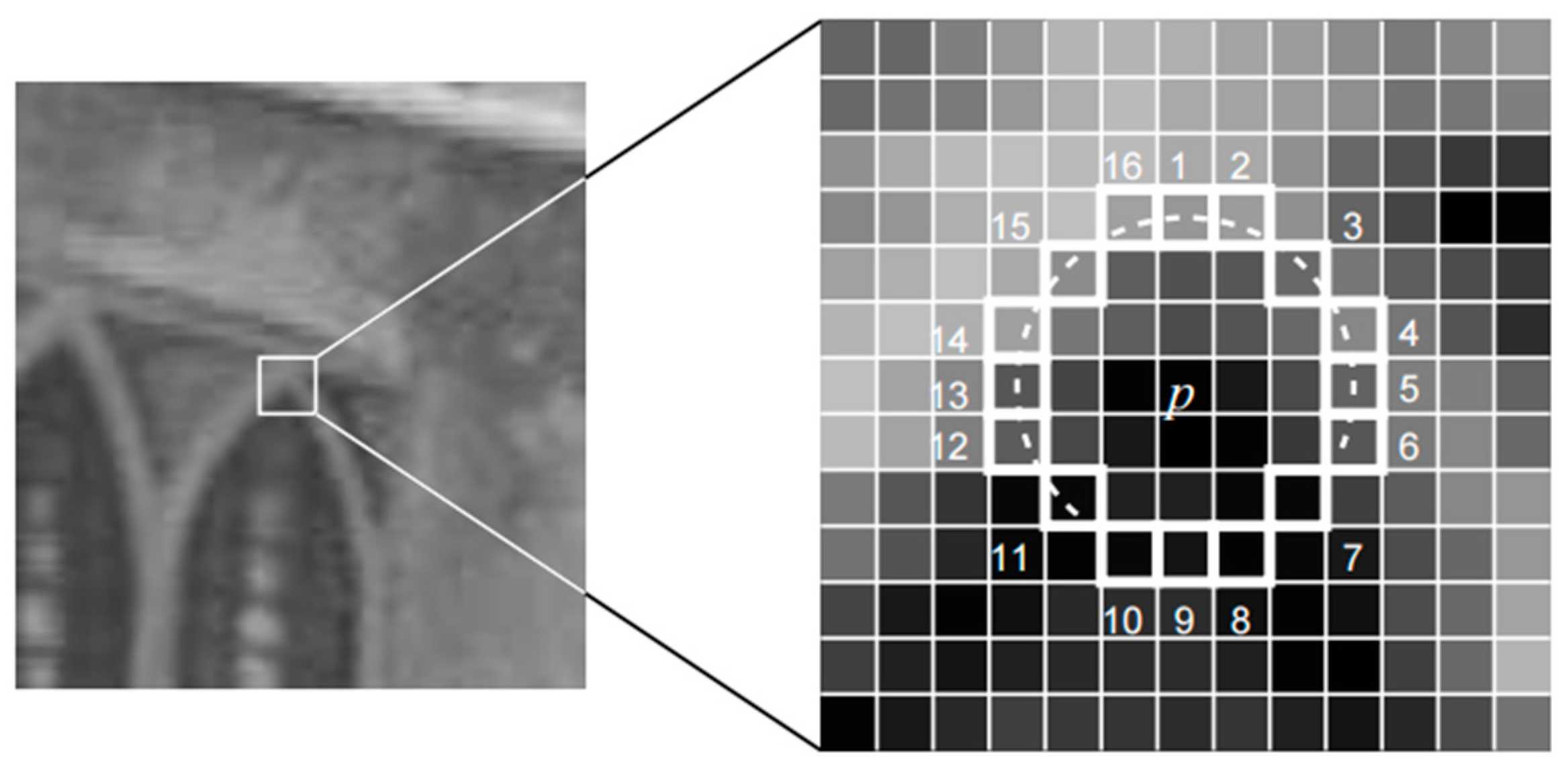
In this regard, the ORB feature points used in the visual SLAM system constructed in this paper are a compromise between accuracy and real-time performance. While appropriately reducing the accuracy of image feature extraction, it has resulted in a significant increase in computational speed to meet the real-time requirements of the visual SLAM algorithm. The ORB feature points consist of an improved FAST corner point and a Binary Robust Independent Element Features (BRIEF) descriptor. The principle of FAST is shown in Figure 2.

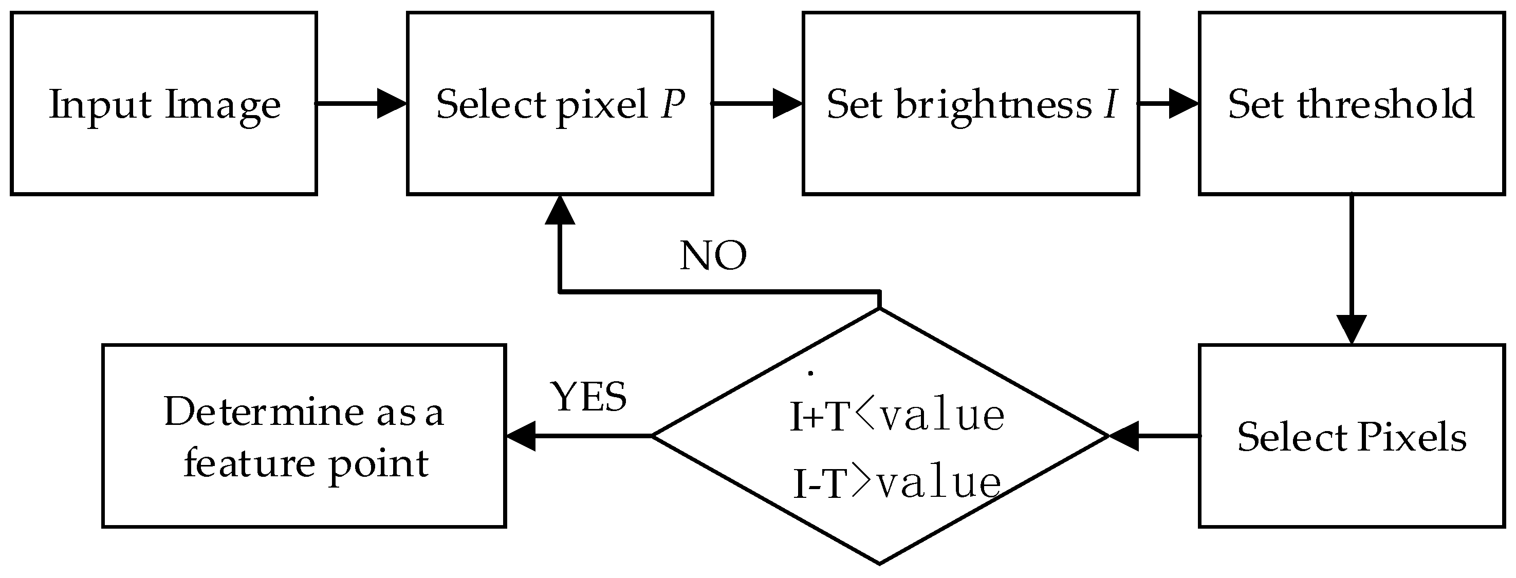
Assuming that there is a pixel $P$ in the image with a brightness of $I$, based on engineering experience, we set a brightness threshold $T$ and select 16 pixels on the circumference with a radius of 3 pixels with a as the center. If there are consecutive $N$ pixels with grayscale values greater than $I+T$ or less than $I-T$, pixel $P$ is considered a corner. The overall FAST corner extraction algorithm process is shown in Figure 3. The ORB algorithm uses an image pyramid to downsample the image and then uses the gray centroid method to solve the problem of image rotation. The centroid refers to taking a gray value as the center of weight. Firstly, the moment of an image is defined as follows:

$$m_{pq}={\displaystyle \sum x^p{y}^{q}I\left(x,y\right) p,q=\left\{0,1\right\}}$$

(1)

The centroid of this image can be found through the following equation:

$$C=\left(\frac{m_{10}}{m_{00}},\frac{m_{01}}{m_{00}}\right)$$

(2)

We connect the centroid and geometric center of the image and then use a vector to represent it. Therefore, the direction of a feature point can be defined as:

$$\theta =\arctan \left(m_{01}/m_{10}\right)$$

(3)

After extracting ORB feature points from the image, the step is feature matching. In cases where the number of feature points is not large, brute force matching can be directly used. However, this method requires a lot of time when the number of feature points is large. Therefore, a fast approximate nearest neighbor algorithm can be used to improve the matching speed.

2.3. Feature Point Homogenization

The dense distribution of image feature points in local areas can affect the accuracy of visual odometry, as using only local area data to represent the global area often results in errors. We adopt an improved ORB feature uniform distribution algorithm based on Quadtree for this purpose. This paper mainly improves the feature point extraction and feature description stages. Firstly, the threshold is calculated based on the grayscale values of different pixel neighborhoods, rather than manually setting the threshold to improve the algorithm’s ability to extract feature points in homogeneous image regions. Secondly, an improved Quadtree structure is adopted for feature point management and optimization to improve the distribution uniformity of detected feature points. To prevent excessive node splitting, threshold values are set in each layer of the pyramid image. In the feature description stage, image information included in the grayscale difference is used to obtain more information support and enhance the discriminative power of the feature description. The overall process of the algorithm is shown in Figure 4. The first step is to construct an eight-layer image pyramid. Assuming that the required number of ORB feature points is m, the scale factor is s, and the number of feature points in the first layer is a,

$$a+\frac{1}{s}a+\frac{1}{s^2}a+\frac{1}{s^3}a+\dots +\frac{1}{s^7}a=m$$

(4)

Based on the resolution of the image, each layer of the pyramid image is divided into grids, in order to make the FAST corner distribution more uniform. The next step is to calculate the feature point extraction threshold in each grid. Due to the fixed threshold of the ORB algorithm, it does not consider the specific situation of the local neighborhood of pixels. Therefore, the feature points detected by the ORB algorithm are concentrated in areas with significant changes in the image, and there are a large number of redundant feature points. For uniform areas of the image, due to the similarity of the grayscale features, the FAST algorithm can only extract a small number of feature points.

In this regard, this paper adopts a dynamic local threshold method. We set a separate threshold t within each grid, and the calculation formula is as follows:

$$t=\alpha \times \left(\frac{1}{m}{\displaystyle \sum _{i=1}^m\left|f\left(Q_i\right)-\overline{f\left(Q\right)}\right|}\right)$$

(5)

Here, $\alpha$ is the scaling factor, usually set to 1.2 based on engineering experience, m is the number of pixels in the grid, $f\left(Q_i\right)$ is the grayscale value of pixels in the grid, and $\overline{f\left(Q\right)}$ is the average grayscale value of all pixels in the grid.

After using dynamic thresholding to extract FAST corners, a relatively uniform distribution of feature points can be obtained, but there is a large number of redundant feature points. Therefore, for this paper, a Quadtree structure is used to further screen feature points. Quadtree, also known as Q-tree, has a maximum of four subnodes per node. Using a Quadtree structure, a two-dimensional space can be divided into four quadrants, and the information in a quadrant can be stored in a subnode. The Quadtree structure is shown in Figure 5. If the number of feature points in a subregion is greater than 1, the splitting will continue in each subregion, while regions without feature points will delete a subnode until the number of nodes equals 1 or reaches the required number of feature points for the system.

The original ORB feature descriptor only uses the size of grayscale values, without using the difference information between grayscale values, resulting in the loss of some image information. In this regard, this paper adopts a feature description method that integrates grayscale difference information, while using grayscale value size and grayscale difference information to describe feature points. Suppose there is a feature point Q; according to the rules of BRIEF algorithm, we select the T group of pixel block pairs to compare the gray value, obtain a binary code string $G_a$, and then record the gray difference of each pixel block pair to generate another binary code string. Assuming $D_w$ is the dataset for recording grayscale differences,

$$G={\left\{G_t\right\}}_{t=1\dots T}={\left\{\left|f\left(A_t\right)-f\left(B_t\right)\right|\right\}}_{t=1\dots T}$$

(6)

Here, f is the average grayscale value of the pixel block. Then, we calculate the average value $G_a$ of these T differences as the threshold for binary encoding these grayscale differences, and the calculation formula is (7). We compare these T grayscale differences with $G_a$, as shown in Formula (8), and then obtain a binary string $D_w^{\wedge }$, as shown in Formula (9). Finally, we combine $D_w$ and $D_w^{\wedge }$ to form a new feature descriptor $D_k$, as shown in Formula (10).

$$G_a=\frac{G}{T}=\frac{1}{T}{\displaystyle \sum _{1\le t\le T}^t{G}_t}$$

(7)

$$h\left(Q,G_t\right)=\{\begin{array}{cc}1& G_t>G_a\\ 0& G_t<G_a\end{array}$$

(8)

$$D_w^{\wedge }={\displaystyle \sum _{1\le t\le T}^t{2}^{t}h\left(Q,G_t\right)}$$

(9)

$$D_k=D_w+D_w^{\wedge }$$

(10)

2.4. Feature Matching

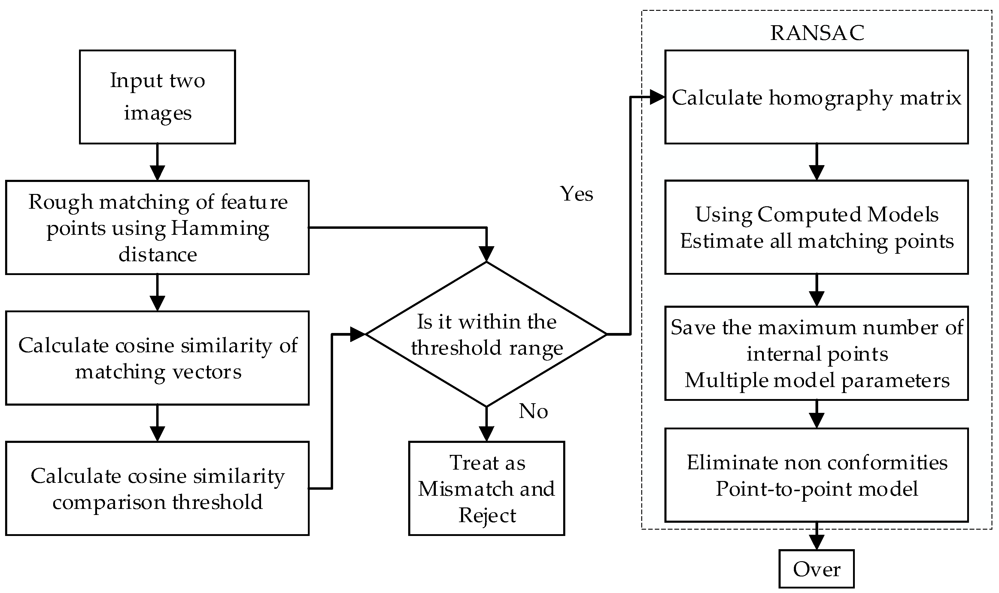
In traditional ORB feature-matching methods, feature vectors are matched by comparing binary strings without considering the correlation between the components of the feature vectors. Therefore, when there are similar regions in the image, there will be more feature mismatches, such as two document images with multiple identical characters. The Hamming distance represents the difference in numerical features between two vectors, which can effectively determine whether two vectors are similar but does not have the ability to describe the directional features of two vectors. We adopt an ORB feature-matching algorithm that combines Hamming distance and cosine similarity. Firstly, we use Hamming distance for coarse matching, then we use cosine similarity for further filtering, and finally we use the Random Sample Consistency (RANSAC) algorithm to further eliminate mismatches. The overall framework of the algorithm is shown in Figure 6.

The algorithm first performs a preliminary screening of ORB feature points waiting for matching based on Hamming distance and then calculates cosine similarity based on this. Assuming there are two ORB feature description vectors a and b, the cosine similarity between them can be obtained:

$$\cos \left(\theta \right)=\frac{\mathit{a}. \mathit{b}}{\Vert \mathit{a}\Vert \times \Vert \mathit{b}\Vert }$$

(11)

Here, the larger the cosine similarity value, the closer the directions of the two vectors are.

The next step is to calculate the comparison threshold for cosine similarity. The specific method is to subtract the cosine similarity of all feature point pairs and then find the value with the highest occurrence frequency from it as the cosine similarity comparison threshold for this feature matching. Considering the existence of errors, a floating value is usually set to 0.3 based on engineering experience. Next, the ORB feature points can be re-filtered based on the cosine similarity comparison threshold, and those feature point pairs that are not within the threshold range can be removed.

Finally, we use the RANSAC algorithm to remove the mismatched feature pairs. Although the previous steps can ensure that most of the matches are correct, there may still be some cases of mismatches. Because these two methods are based on the local characteristics of the image, it is necessary to remove the mismatched feature pairs from the perspective of the entire image. The RANSAC algorithm can eliminate outliers in a dataset by calculating the best model of the data which are also known as outer points, and it can retain normal values that conform to this model, which are also known as inner points.

The algorithm first randomly selects four pairs of feature points from the dataset and then calculates the homography matrix H, which is the initialization of the optimal model. We use the homography matrix H to test all data. If the error between the coordinate point and the actual result obtained through homography matrix transformation is small enough, then the point is considered an interior point. If there are not enough internal points, we select new random points and recalculate the new homography matrix model until the internal points are sufficient. The minimum number of iterations k of the RANSAC algorithm should meet the following:

$$\{\begin{array}{l}1-P_m={\left(1-{\eta }^m\right)}^k\\ k=\frac{\ln \left(1-P_m\right)}{\ln \left(1-{\eta }^m\right)}\end{array}$$

(12)

Here, the minimum amount of data required to calculate the homography matrix H is m; $P_m$ is the confidence level, representing the probability of at least one inner point in m ORB feature point pairs; and $\eta$ represents the probability of the selected ORB feature point pair being an outer point.

2.5. Camera Pose Estimation

After the ORB feature extraction and matching steps described in the previous section, a correctly matched and evenly distributed pair of feature points can be obtained, and then the camera motion can be estimated based on this. The Iterative Closest Point (ICP) algorithm can calculate the camera’s pose changes based on two RGB-D images. Assuming that after the feature-matching step, there is a set of paired 3D points,

$$\{\begin{array}{l}\mathit{P}=\left\{{\mathit{p}}_1,\dots ,{\mathit{p}}_n\right\}\\ {\mathit{P}}^{\prime }=\left\{{\mathit{p}}_1^{\prime },\dots ,{\mathit{p}}_n^{\prime }\right\}\end{array}$$

(13)

According to the camera rigid body motion theory, the camera motion can be represented by the rotation matrix R and the translation vector t:

$$\forall i,{\mathit{p}}_i=\mathit{R}{\mathit{p}}_i^{\prime }+\mathit{t}$$

(14)

The ICP algorithm constructs the solution process of camera motion into a least-square form, assuming that the error between the matched ORB feature points is

$${\mathit{e}}_i={\mathit{p}}_i-\left(\mathit{R}{\mathit{p}}_i^{\prime }+\mathit{t}\right)$$

(15)

This error term is constructed into a least-square problem, and the camera position and pose at this time can be obtained by minimizing the sum of error squares:

$$\min f\left(\mathit{R},\mathit{t}\right)=\frac{1}{2}{{\displaystyle \sum _{n=1}^n\Vert {\mathit{p}}_i-\left(\mathit{R}{\mathit{p}}_i^{\prime }+\mathit{t}\right)\Vert }}^2$$

(16)

Before solving Formula (16), we define the centroids of these two matched ORB feature points and then simplify the formula through the centroids:

$$\{\begin{array}{l}\mathit{p}=\frac{1}{n}{\displaystyle \sum _{i=1}^n{\mathit{p}}_i}\\ {\mathit{p}}^{\prime }=\frac{1}{n}{\displaystyle \sum _{i=1}^n{\mathit{p}}_i^{\prime }}\end{array}$$

(17)

$$\min f\left(\mathit{R},\mathit{t}\right)=\frac{1}{2}{\displaystyle \sum _{n=1}^n{\Vert {\mathit{p}}_i-\mathit{p}-\mathit{R}\left({\mathit{p}}_i^{\prime }-{\mathit{p}}^{\prime }\right)\Vert }^2+}{\Vert \mathit{p}-\left(\mathit{R}{\mathit{p}}_i^{\prime }+\mathit{t}\right)\Vert }^2$$

(18)

where the left term on the right side of the equation is only related to the rotation matrix R. If the rotation matrix R is known, we order the right term on the right side of the equation to be equal to 0 to obtain the translation vector t. So, ICP can be solved in three steps, first calculating the centroid coordinates of these two matched ORB feature points:

$$\{\begin{array}{l}{\mathit{q}}_i={\mathit{p}}_i-\mathit{p}\\ {\mathit{q}}_i^{\prime }={\mathit{p}}_i^{\prime }-{\mathit{p}}^{\prime }\end{array}$$

(19)

Then, the second step is to calculate the rotation matrix R according to Formula (20), and the last step is to obtain the translation vector t according to Formula (21):

$$\mathit{R}=\arg \underset{\mathit{R}}{\min }\frac{1}{2}{\displaystyle \sum _{i=1}^n{\Vert {\mathit{q}}_i-\mathit{R}{\mathit{q}}_i^{\prime }\Vert }^2}$$

(20)

$$\mathit{t}=\mathit{p}-\mathit{R}{\mathit{p}}^{\prime }$$

(21)

3. Experimental Environment and Datasets

The data processing platform for this experiment was an Intel (R) Core (TM) i3-8100M CPU @ 2.60GHz main frequency, 16GB memory laptop, running the Ubuntu 16.04 operating system. The development software was Microsoft Visual Studio 2019 and the image algorithm library OpenCV 2.4.10, and the programming was implemented in C++ language.

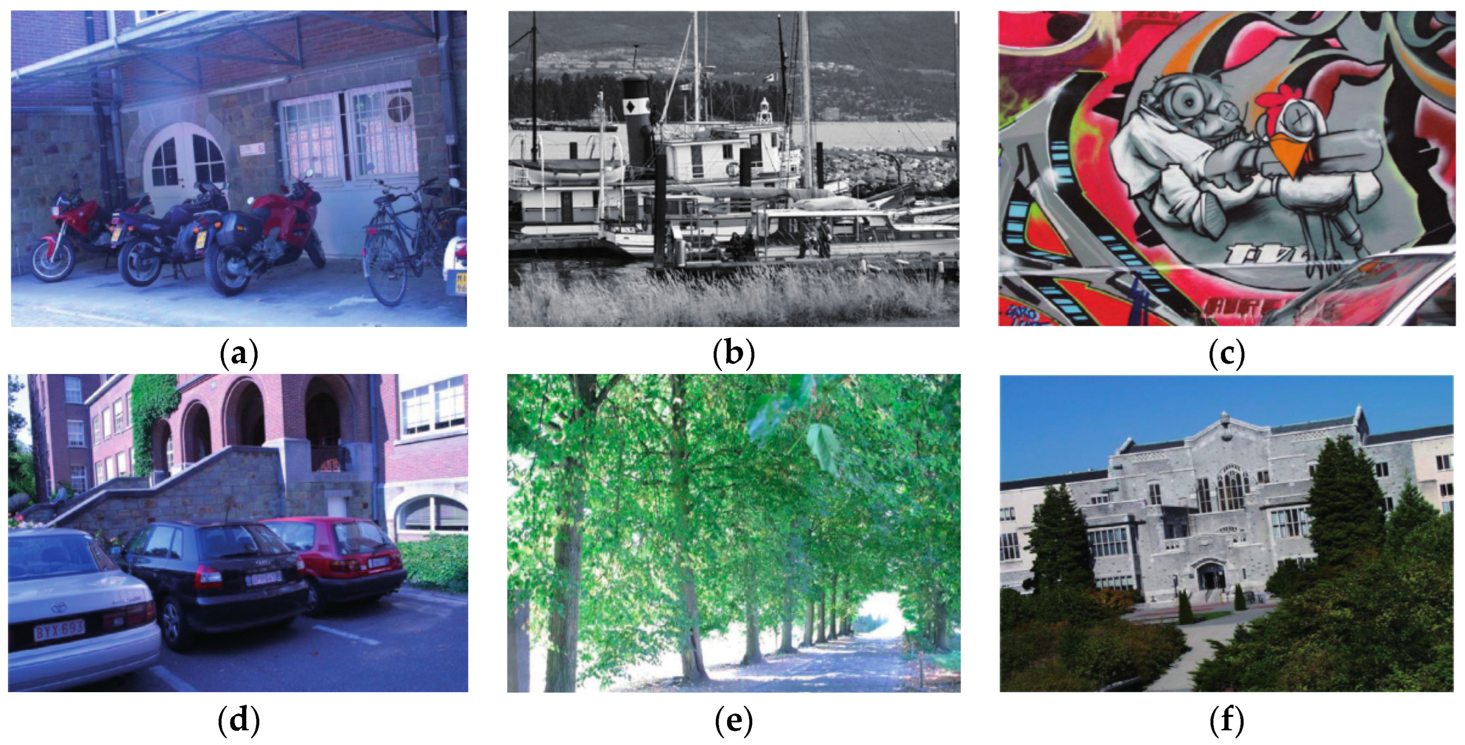
In the experiments of feature extraction, homogenization, and feature matching, the test image data were obtained using the Oxford Optical Image Dataset provided by Schmid, which includes multiple image categories [24], including images with different lighting intensities, perspectives, blurring levels, and resolutions, as shown in Figure 7. The Trees dataset contains a set of images with complex textures. The images in the Bikes dataset have varying degrees of blur, the compression of the Ubc dataset is different, the contrast of the Leuven dataset is different, and the images in the Boat dataset are rotated to a certain extent.

The TUM dataset released by the Computer Vision Laboratory of the Technical University of Munich as experimental data [25] was used in the localization and mapping experiment. This dataset is composed of multiple image sequences collected by a depth camera in two different indoor environments. Each image sequence contains color images and depth images, as well as the real camera motion track collected by the motion capture system, which is the GroundTruth.txt file in the dataset folder. In addition, the dataset is time-synchronized with the motion capture system based on camera calibration. This experiment uses three image sequences from the TUM dataset, namely fr1/xyz, fr1/desk, and fr1/desk2. Among them, fr1/xyz contains a set of image sequences recorded by a handheld depth camera, which only performs slow translation motion in the main axis direction, making it more suitable for evaluating trajectory accuracy. In the fr1/desk scene, an office environment is set up, which includes two desks with computer monitors, keyboards, books, and other objects. The environment texture is relatively rich, and it describes the scene where a handheld depth camera surrounds the desk for a week. Compared to fr1/desk, although the scene is the same, fr1/desk2 contains more objects, and the camera moves faster. The detailed information on the three datasets selected for the experiment is shown in

Table 1. Test Dataset Details.

Sequence	Trajectory Length	Number of Frames	Average Angular Velocity	Translational Speed
fr1/xyz	7.11 m	798	8.920 deg/s	0.244 m/s
fr1/desk	18.88 m	2965	23.33 deg/s	0.293 m/s
fr1/desk2	10.16 m	640	29.31 deg/s	0.430 m/s

.

4. Technical Implementation and Results

4.1. Feature Point Extraction and Homogenization

In order to verify the effectiveness of the uniform ORB algorithm based on a dynamic threshold and improved Quadtree proposed in Section 2 of this paper, an experimental analysis was carried out from the two aspects of feature point distribution uniformity and calculation efficiency. Six image groups were selected from the Oxford dataset for experimentation, namely Bikes (blur), Boat (rotation and scaling), Graf (viewpoint), Leuven (illumination), Trees (blur), and Ubc (JPG compression). As a comparison, two types of feature point algorithms were used for comparative experiments, namely the feature point algorithm based on floating-point feature description and the feature point algorithm based on binary feature description.

The algorithms based on floating-point feature description include SIFT and SURF, while the algorithms based on binary feature description include ORB and the methods used in ORB-SLAM (represented by the symbol MRA in this paper). Finally, to ensure the generality of the test results, 30 experiments were conducted on each set of image datasets, with the average value as the final experimental result.

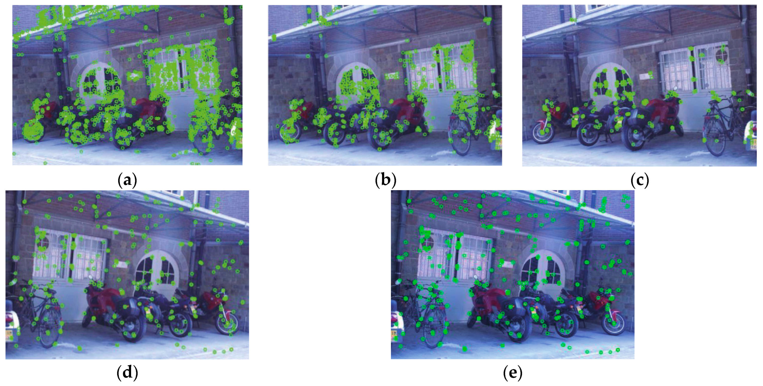
Firstly, the performance differences in the uniform distribution of feature points among these five algorithms can be intuitively observed through observation. Figure 8 shows the feature point extraction results of the Bikes image dataset using the Oxford dataset. It can be seen that the feature points extracted by SIFT, SURF, and the original ORB algorithm are less evenly distributed than those extracted by MRA and the algorithm in this paper, and they are more concentrated in areas with obvious local areal feature characteristics of the image, such as doors and windows, which are more prominent edge image areas; however, there are not many feature points extracted in homogeneous areas such as walls. The feature points extracted by MRA and our algorithm are significantly more evenly distributed than those extracted by other algorithms. Compared with the MRA algorithm, the method proposed in this paper can extract feature points that MRA cannot extract in areas where the image features are not obvious, such as the wall area in the upper right corner of the image.

In order to quantify the distribution of feature points, a feature point distribution uniformity function is used, where a smaller uniformity value indicates a more uniform distribution of feature points. The experimental results are shown in

Table 2. Average uniformity of characteristic points of five algorithms on Oxford dataset.

Algorithm	SIFT	SURF	ORB	MRA	This Paper
Bikes	189.54	254.09	171.85	141.27	140.64
Boat	201.34	201.34	148.83	111.05	92.43
Graf	158.66	159.55	120.23	84.45	84.37
Leuven	234.04	273.04	175.45	158.66	168.16
Trees	206.39	231.24	146.66	112.15	113.32
Ubc	253.76	269.88	180.09	168.16	166.01

.

Among the six scenes in the Oxford image dataset, the uniformity values of MRA and our algorithm are smaller, indicating a more uniform distribution of feature points. Meanwhile, compared to MRA, our algorithm can be applied to more scenarios. For example, in the boat image group, our algorithm has improved uniformity by about 17% compared to MRA, indicating that our algorithm has a higher tolerance for image rotation and scaling. Compared to the original ORB algorithm, our algorithm has improved uniformity by 53%.

4.2. Feature Matching and Mismatching Elimination

The content of this section is the verification of the effectiveness of the improved ORB matching algorithm based on cosine similarity proposed in Section 2.4 of this paper. The evaluation criterion is feature-matching accuracy.

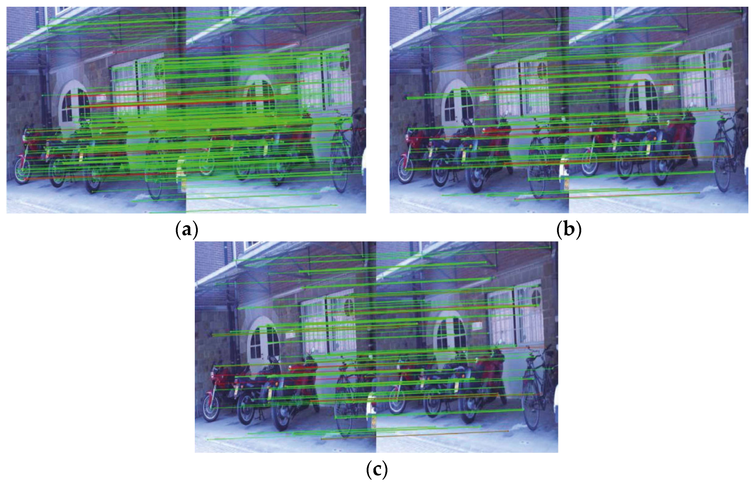
The experiment used three algorithms for comparison, namely the original ORB algorithm, the method used in ORB-SLAM (represented by the symbol MRA in this paper), and the improved algorithm proposed by the authors. Figure 9 shows the ORB feature point matching results of the Bikes image dataset using the Oxford dataset. The feature points connected by green lines represent correct feature matching, while the red lines represent mismatching. From the feature point matching results of the three algorithms, it can be seen that MRA and our algorithm have fewer red lines, indicating fewer mismatching phenomena.

To ensure the generality of the test results, 30 experiments were conducted on each set of image datasets, with the average value as the final experimental result, and the average accuracy is shown in

Table 3. Average matching accuracy of feature points of three algorithms on different datasets.

Algorithm	Bikes	Boat	Graf	Leuven	Trees	Ubc
ORB	58.04	50.95	39.46	63.90	73.64	68.66
MRA	70.55	64.31	46.45	86.84	90.43	85.56
Our algorithm	76.52	76.39	47.18	88.90	94.37	90.45

. From the experimental results, it can be seen the matching accuracy of MRA and our algorithm on these six image sets is higher than that of the original ORB algorithm. Compared with MRA, our algorithm does not have much difference in feature-matching accuracy on the Bikes, Graf, Leuven, and Ubc datasets, but it has significantly improved matching accuracy on the Boat dataset. The reason is that our algorithm uses cosine similarity to screen the matching point pairs after the initial matching of Hamming distance, removing some mismatched point pairs caused by image rotation. After calculation, compared with the original ORB algorithm, the average feature-matching accuracy of our algorithm on six datasets has been improved by 33%. Compared with MRA, the average feature-matching accuracy of our algorithm on six datasets has been improved by 6.5%, and the ORB feature-matching algorithm proposed in this thesis has a higher tolerance for image rotation.

4.3. Localization and Map Construction

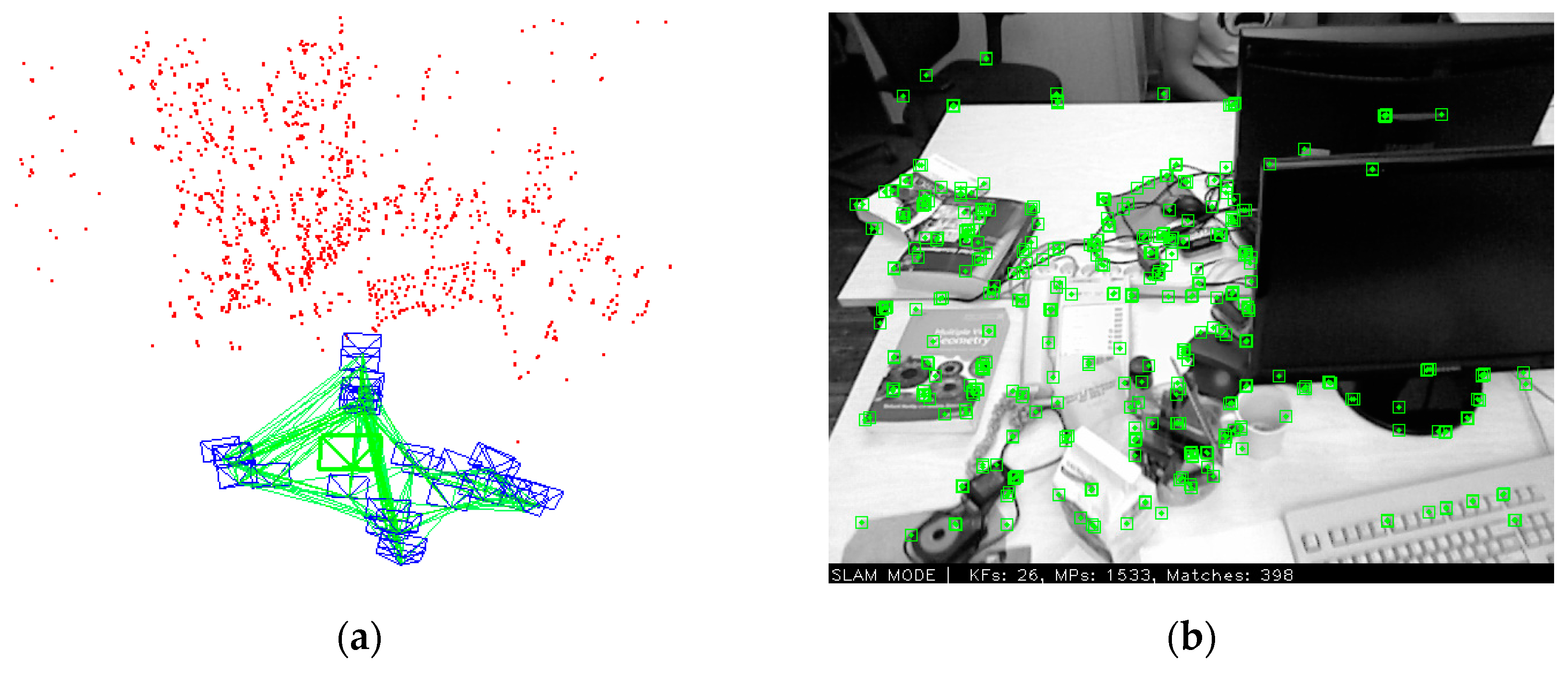
In order to verify the performance of the visual-information-based autonomous localization system constructed in this paper, simulation experiments were conducted using partial sequences from the TUM dataset. For the convenience of representation, the algorithm in this paper was named My-SLAM. As the algorithm in this paper was improved on the ORB-SLAM algorithm framework, comparative simulation experiments were conducted using the ORB-SLAM algorithm. The results of the algorithm proposed in this paper running on the fr1/xyz sequence are shown in Figure 10. The red points in Figure 10a represent the ORB feature points projected onto the map, and the green lines and blue boxes represent the camera’s pose changes and the camera’s position in three-dimensional space, respectively. Figure 10b shows the real-time ORB feature point extraction results of the visual odometer module.

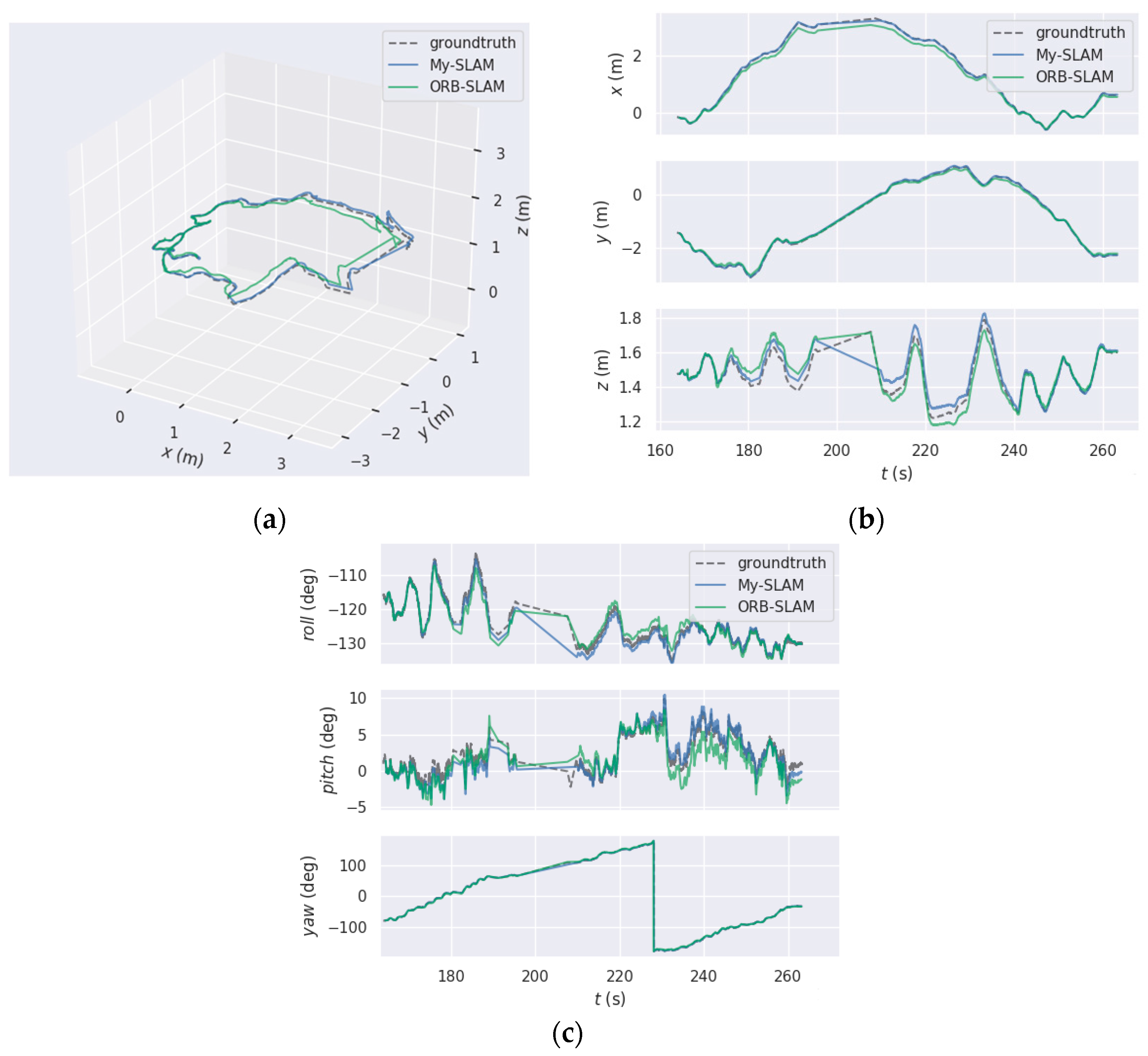
In order to evaluate the trajectory accuracy estimated by the algorithm in this paper, a comparative experimental analysis was conducted with ORB-SLAM on the fr1/xyz sequence and fr1/desk sequence, and the results are shown in Figure 11 and Figure 12. From Figure 11 and Figure 12a, it can be intuitively seen that the camera motion trajectory estimated by the algorithm in this paper is closer to the real trajectory than the ORB-SLAM algorithm. For further data analysis, this paper will decompose the camera’s motion from two angles: the translational motion in the main axis direction and the azimuth angle. Firstly, the translational motion in the main axis direction is considered. The experimental results are shown in Figure 11 and Figure 12b. For example, in the fr1/desk sequence, although there is not much difference between the two algorithms in the X-axis and Y-axis directions, the algorithm in this paper has higher accuracy than ORB-SLAM in the Z-axis direction. From the comparison of azimuth angles shown in Figure 11 and Figure 12c, it can be seen that although the motion trajectories of the two algorithms are basically the same at the beginning of a period of time, as the running time increases, the ORB-SLAM algorithm begins to experience trajectory errors. In contrast, the trajectory errors observed in the proposed method are smaller, indicating better stability of the proposed algorithm.

The algorithms in this paper are evaluated from a quantitative perspective. The APE and RPE of the two algorithms on three dataset sequences are calculated, and then their root-mean-square error (RMSE) is calculated. The experimental results are shown in

Table 4. RMSE comparison of RPE of two algorithms.

Algorithm	fr1/xyz	fr1/Desk2	fr1/Desk
My-SLAM	0.0126 m	0.0582 m	0.0191 m
ORB-SLAM	0.0139 m	0.0752 m	0.0223 m

and

Table 5. RMSE comparison of APE of two algorithms.

Algorithm	fr1/xyz	fr1/Desk2	Fr1/Desk
My-SLAM	0.0109 m	0.0439 m	0.0247 m
ORB-SLAM	0.0121 m	0.0533 m	0.0296 m

. Firstly, there is a comparison of the RMSE of the RPE of the two algorithms. In the fr1/xyz sequence where the camera only moves slowly along the main axis, the RMSE of our algorithm is not significantly different from that of the original ORB-SLAM algorithm. However, in the fr1/desk series dataset where the camera moves faster and the scene is more complex, the error of our algorithm is significantly smaller than that of the ORB-SLAM algorithm. It can also be seen from the RMSE comparison experiment results of APE of the two algorithms that with the increase in the complexity of dataset scenes and the change in camera attitude, the increase in the RMSE of the algorithm in this paper is smaller than that of ORB-SLAM. In order to further investigate the relationship between the localization errors of the two algorithms in different datasets, the percentage reduction in localization errors of our algorithm compared to ORB-SLAM in different datasets was calculated. After calculation, the average RPE of our algorithm on the three datasets was reduced by 15.4% compared to ORB-SLAM, while the average APE was reduced by 13.9% compared to ORB-SLAM.

5. Discussion and Future Work

In the indoor environment where GPS signals are missing, mobile robots cannot use satellite signals to determine their own positions, which greatly limits the application scenarios for mobile robots. This article proposes a method for indoor positioning of mobile robots based on depth cameras. The localization algorithm is mainly divided into three parts, namely ORB feature extraction, feature matching, and pose estimation.

In the ORB feature extraction section, due to the uneven distribution of feature points extracted by the original ORB algorithm, the dense distribution of feature points in local areas of the image will degrade the accuracy of subsequent pose estimation. In this regard, this paper proposes an improved Quadtree feature extraction algorithm based on a dynamic threshold, which uses the Quadtree structure to divide the image into regions and then calculates the FAST corner comparison threshold in each sub-region to achieve a uniform distribution of ORB feature points. The comparative experimental results are shown in Table 2. For example, in the boat image group, our algorithm improved uniformity by about 17% compared to MRA, indicating that our algorithm has a higher tolerance for image rotation and scaling. Compared with the original ORB algorithm, our algorithm improves consistency by 53%.

In the ORB feature-matching part, the mismatching between feature points will affect the final positioning accuracy. We combined the feature-matching method based on Hamming distance with cosine similarity and conducted a secondary screening of the results after the initial feature matching, and then we used the RANSAC algorithm to eliminate the external points of the feature points without matching from the global perspective. Figure 9c shows the improved feature-matching results. Compared with the original ORB algorithm, our algorithm improves the average feature-matching accuracy by 33% on six datasets. Compared with ORB-SLAM, our algorithm has an average feature-matching accuracy improvement of 6.5% on six datasets, and the ORB feature-matching algorithm proposed in this paper has a higher tolerance for image rotation. All experimental results are shown in Table 3.

The improvement of feature extraction and matching is the main reason for the improved accuracy of the overall positioning algorithm. We compared the algorithm proposed in this paper with ORB-SLAM on three TUM datasets and calculated their average positioning accuracy after multiple experiments. The results are shown in Table 4 and Table 5. Compared with ORB-SLAM, our algorithm achieved an average RPE reduction of 15.4% and an average APE reduction of 13.9% on the three datasets.

Through experiments, it was found that although the algorithm in this paper runs relatively smoothly most of the time, its positioning accuracy is poor during intense camera motion, which is a disadvantage of all pure visual SLAM methods. Therefore, in our future work, we will consider integrating inertial sensors, which can adapt to intense movements in a short period of time. Combining the two approaches can effectively improve the accuracy and robustness of the positioning algorithm.

6. Conclusions

This paper presents a depth-camera-based positioning system for the indoor positioning of mobile robots as the application background. The algorithm is mainly divided into four parts, namely the feature extraction module, feature point homogenization module, feature-matching module, and pose estimation module. In the feature extraction module, in order to balance accuracy and real-time performance, ORB feature points are used. In the ORB feature extraction module of the algorithm, in view of the poor uniformity of the traditional ORB algorithm, an improved ORB feature uniform distribution algorithm based on Quadtree is used for this paper. In the feature-matching module of the algorithm, an improved ORB algorithm based on cosine similarity is proposed to address the problem of a high mismatch rate when ORB matches images with multiple similar regions. With the foundation of the first three steps, the ICP algorithm is used in the pose estimation module to estimate the camera’s pose. The final experimental results indicate that the average positioning accuracy of our algorithm in three indoor scenes on the TUM dataset is 0.027 m, which can meet the needs of autonomous positioning for mobile robots.

References

1. Ohno, K.; Tsubouchi, T.; Shigematsu, B. Differential GPS and odometry-based outdoor navigation of a mobile robot. Adv. Robot. 2004, 18, 611–635. [Google Scholar] [CrossRef]
2. Khan, M.U.; Zaidi, S.A.A.; Ishtiaq, A.; Bukhari, S.U.R.; Samer, S. A comparative survey of lidar-slam and lidar based sensor technologies. In Proceedings of the 2021 Mohammad Ali Jinnah University International Conference on Computing, Karachi, Pakistan, 15–17 July 2021; pp. 1–8. [Google Scholar]
3. Van der Kruk, E.; Marco, M.; Reijne, M.M. Accuracy of human motion capture systems for sport applications; state-of-the-art review. Eur. J. Sport Sci. 2018, 18, 806–819. [Google Scholar] [CrossRef] [PubMed]
4. Zafari, F.; Gkelias, A.; Leung, K.K. A survey of indoor localization systems and technologies. IEEE Commun. Surv. Tutor. 2019, 21, 2568–2599. [Google Scholar] [CrossRef]
5. Balasuriya, B.; Chathuranga, B.; Jayasundara, B.; Napagoda, N.; Kumarawadu, S.; Chandima, D.; Jayasekara, A. Outdoor robot navigation using Gmapping based SLAM algorithm. In Proceedings of the 2016 Moratuwa Engineering Research Conference, Moratuwa, Sri Lanka, 4–5 April 2016; pp. 403–408. [Google Scholar]
6. Wei, W.; Shirinzadeh, B.; Ghafarian, M.; Esakkiappan, S.; Shen, T. Hector SLAM with ICP trajectory matching. In Proceedings of the 2020 IEEE/ASME International Conference on Advanced Intelligent Mechatronics, Boston, MA, USA, 6–10 July 2020; pp. 1971–1976. [Google Scholar]
7. Meng, Z.; Xia, X.; Xu, R. HYDRO-3D: Hybrid Object Detection and Tracking for Cooperative Perception Using 3D LiDAR. IEEE Trans. Intell. Veh. 2023. [Google Scholar] [CrossRef]
8. Liu, W.; Quijano, K.; Crawford, M.M. YOLOv5-Tassel: Detecting tassels in RGB UAV imagery with improved YOLOv5 based on transfer learning. IEEE J. Sel. Top. Appl. Earth Obs. Remote Sens. 2022, 15, 8085–8094. [Google Scholar] [CrossRef]
9. Nützi, G.; Weiss, S.; Scaramuzza, D. Fusion of IMU and vision for absolute scale estimation in monocular SLAM. J. Intell. Robot. Syst. 2011, 61, 287–299. [Google Scholar] [CrossRef]
10. Qin, T.; Li, P.; Shen, S. Vins-mono: A robust and versatile monocular visual-inertial state estimator. IEEE Trans. Robot. 2018, 34, 1004–1020. [Google Scholar] [CrossRef]
11. Saputra, M.R.U.; Markham, A.; Trigoni, N. Visual SLAM and structure from motion in dynamic environments: A survey. ACM Comput. Surv. (CSUR) 2018, 51, 1–36. [Google Scholar] [CrossRef]
12. Taketomi, T.; Uchiyama, H.; Ikeda, S. Visual SLAM algorithms: A survey from 2010 to 2016. IPSJ Trans. Comput. Vis. Appl. 2017, 9, 1–11. [Google Scholar] [CrossRef]
13. Sturm, P. Multi-view geometry for general camera models. In Proceedings of the 2005 IEEE Computer Society Conference on Computer Vision and Pattern Recognition, San Diego, CA, USA, 20 June–26 June 2005; pp. 206–212. [Google Scholar]
14. Macario, B.A.; Michel, M.; Moline, Y. A comprehensive survey of visual slam algorithms. Robotics 2022, 11, 24. [Google Scholar] [CrossRef]
15. Zuo, X.; Xie, X.; Liu, Y. Robust visual SLAM with point and line features. In Proceedings of the 2017 IEEE/RSJ International Conference on Intelligent Robots and Systems (IROS), Vancouver, BC, Canada, 24–29 September 2017; pp. 1775–1782. [Google Scholar]
16. Silveira, G.; Malis, E.; Rives, P. An efficient direct approach to visual SLAM. IEEE Trans. Robot. 2008, 24, 969–979. [Google Scholar] [CrossRef]
17. Smith, R. On the estimation and representation of spatial uncertainty. Int. J. Robot. Res. 1987, 5, 113–119. [Google Scholar] [CrossRef]
18. Davison, A.J.; Reid, I.D.; Molton, N.D.; Stasse, O. MonoSLAM: Real-time single camera SLAM. IEEE Trans. Pattern Anal. Mach. Intell. 2007, 29, 1052–1067. [Google Scholar] [CrossRef] [PubMed]
19. Klein, G.; Murray, D. Parallel tracking and mapping for small AR workspaces. In Proceedings of the 2007 6th IEEE and ACM International Symposium on Mixed and Augmented Reality, Nara, Japan, 13–16 November 2007; pp. 225–234. [Google Scholar]
20. Newcombe, R.A.; Lovegrove, S.J.; Davison, A.J. DTAM: Dense tracking and mapping in real-time. In Proceedings of the 2011 International Conference on Computer Vision, Barcelona, Spain, 6–13 November 2011; pp. 2320–2327. [Google Scholar]
21. Juan, L.; Gwun, O. A comparison of sift, pca-sift and surf. Int. J. Image Process. (IJIP) 2009, 3, 143–152. [Google Scholar]
22. Bay, H.; Ess, A.; Tuytelaars, T.; Van Gool, L. Speeded-up robust features (SURF). Comput. Vis. Image Underst. 2008, 110, 346–359. [Google Scholar] [CrossRef]
23. Rublee, E.; Rabaud, V.; Konolige, K.; Bradski, G. ORB: An efficient alternative to SIFT or SURF. In Proceedings of the 2011 International Conference on Computer Vision, Barcelona, Spain, 6–13 November 2011; pp. 2564–2571. [Google Scholar]
24. Mikolajczyk, K.; Schmid, C. A performance evaluation of local descriptors. IEEE Trans. Pattern Anal. Mach. Intell. 2005, 27, 1615–1630. [Google Scholar] [CrossRef]
25. Sturm, J.; Engelhard, N.; Endres, F.; Burgard, W.; Cremers, D. A benchmark for the evaluation of RGB-D SLAM systems. In Proceedings of the 2012 IEEE/RSJ International Conference on Intelligent Robots and Systems, Vilamoura-Algarve, Portuga, 7–12 October 2012; pp. 573–580. [Google Scholar]
Figure 1. Overall process of localization algorithm.
Remotesensing 15 04016 g001
Figure 2. FAST corner diagram. The parameter p represents a pixel in the image.
Remotesensing 15 04016 g002
Figure 3. FAST corner extraction algorithm flow. Select a pixel p in the image with brightness I and T as the comparison threshold for grayscale values.
Remotesensing 15 04016 g003
Figure 4. Overall process of feature point homogenization algorithm.
Remotesensing 15 04016 g004
Figure 5. Schematic diagram of Quadtree structure. (a) Regional quadrant division; (b) Quadtree node distribution.
Remotesensing 15 04016 g005
Figure 6. Overall process of Random Sample Consistency (RANSAC) algorithm.
Remotesensing 15 04016 g006
Figure 7. Oxford Optical Dataset. (a) Bikes; (b) Boat; (c) Graf; (d) Leuven; (e) Trees; (f) Ubc.
Remotesensing 15 04016 g007
Figure 8. The feature point extraction results of five algorithms on the Bikes image dataset of Oxford dataset. (a) SIFT; (b) SURF; (c) ORB; (d) MRA; (e) algorithm proposed in this paper.
Remotesensing 15 04016 g008
Figure 9. ORB feature point matching results of three algorithms on Bikes image dataset of Oxford dataset. (a) ORB; (b) MRA; (c) proposed algorithm.
Remotesensing 15 04016 g009
Figure 10. The running results of this algorithm on the fr1/xyz sequence of TUM. (a) The change in camera position and posture and its motion track; (b) ORB feature extraction.
Remotesensing 15 04016 g010
Figure 11. Experimental results of two algorithms on the fr1/xyz sequence of TUM. (a) Overall track map; (b) track change in spindle direction; (c) change in azimuth.
Remotesensing 15 04016 g011aRemotesensing 15 04016 g011b
Figure 12. Experimental results of two algorithms on the fr1/desk sequence of TUM. (a) Overall track map; (b) track change in spindle direction; (c) change in azimuth.
Remotesensing 15 04016 g012