Article

Estimation of High-Resolution Soil Moisture in Canadian Croplands Using Deep Neural Network with Sentinel-1 and Sentinel-2 Images

1
Geomatics Research Institute, Pukyong National University, Busan 48513, Republic of Korea
2
Department of Spatial Information Engineering, Pukyong National University, Busan 48513, Republic of Korea
3
Department of Water Resources, Graduate School of Water Resources, Sungkyunkwan University, Suwon 16419, Republic of Korea
4
Department of Applied Plant Science, Chonnam National University, Gwangju 61186, Republic of Korea
*
Author to whom correspondence should be addressed.
Remote Sens. 2023, 15(16), 4063; https://doi.org/10.3390/rs15164063
Submission received: 24 June 2023 / Revised: 12 August 2023 / Accepted: 15 August 2023 / Published: 17 August 2023
(This article belongs to the Special Issue Remote Sensing for Soil Moisture and Vegetation Parameters Retrieval)

Abstract

:
Soil moisture (SM) is a crucial hydrologic factor that affects the global cycle of energy, carbon, and water, as well as plant growth and crop yield; therefore, an accurate estimate of SM is important for both the global environment and agriculture. Satellite-based SM data have been provided by the National Aeronautics and Space Administration (NASA)’s Soil Moisture Active Passive (SMAP) and the European Space Agency (ESA)’s Soil Moisture and Ocean Salinity (SMOS) satellite missions, but these data are based on passive microwave sensors, which have limited spatial resolution. Thus, detailed observations and analyses of the local distribution of SM are limited. The recent emergence of deep learning techniques, such as rectified linear unit (ReLU) and dropout, has produced effective solutions to complex problems. Deep neural networks (DNNs) have been used to accurately estimate hydrologic factors, such as SM and evapotranspiration, but studies of SM estimates derived from the joint use of DNN and high-resolution satellite data, such as Sentinel-1 and Sentinel-2, are lacking. In this study, we aim to estimate high-resolution SM at 30 m resolution, which is important for local-scale SM monitoring in croplands. We used a variety of input data, such as radar factors, optical factors, and vegetation indices, which can be extracted from Sentinel-1 and -2, terrain information (e.g., elevation), and crop information (e.g., cover type and month), and developed an integrated SM model across various crop surfaces by using these input data and DNN (which can learn the complexity and nonlinearity of the various data). The study was performed in the agricultural areas of Manitoba and Saskatchewan, Canada, and the in situ SM data for these areas were obtained from the Agriculture and Agri-Food Canada (AAFC) Real-time In Situ Soil Monitoring for Agriculture (RISMA) network. We conducted various experiments with several hyperparameters that affected the performance of the DNN-based model and ultimately obtained a high-performing SM model. The optimal SM model had a root-mean-square error (RMSE) of 0.0416 m3/m3 and a correlation coefficient (CC) of 0.9226. This model’s estimates showed better agreement with in situ SM than the SMAP 9 km SM. The accuracy of the model was high when the daily precipitation was zero or very low and also during the vegetation growth stage. However, its accuracy decreased when precipitation or the vitality of the vegetation were high. This suggests that precipitation affects surface erosion and water layer formation, and vegetation adds complexity to the SM estimate. Nevertheless, the distribution of SM estimated by our model generally reflected the local soil characteristics. This work will aid in drought and flood prevention and mitigation, and serve as a tool for assessing the potential growth of crops according to SM conditions.

1. Introduction

Soil moisture (SM) refers to the amount of water in the active layer of top soil [1]. It is a key hydrological parameter affecting global cycles (climate, hydrology, and carbon), crop yields, and disasters, such as droughts and floods. SM determines the amount of latent heat and heat released through evapotranspiration during the Earth’s energy cycle [2], and also affects the atmospheric variability that occurs between the near surface and the atmosphere [3,4]. Additionally, SM is an essential factor for the survival of plants and microorganisms, as it affects photosynthesis, respiration, and microbial activities, thereby influencing the carbon cycle [5]; it is also used to monitor drought and predict crop production [6]. SM also plays a role in determining rainfall infiltration and runoff, thereby enabling flood monitoring [6,7].
SM is typically observed using equipment such as time-domain reflectometry (TDR) and Stevens HydraProbe sensors installed in the soil [8,9]. However, these in situ observation techniques are prohibitively expensive for observing the spatial distribution of SM over large areas [10]. In contrast, satellite-based SM data are useful for confirming the continuous spatial and temporal distribution of SM. These data are currently provided by the Soil Moisture and Ocean Salinity (SMOS) mission of the European Space Agency (ESA) and the Soil Moisture Active Passive (SMAP) mission of the National Aeronautics and Space Administration (NASA). The SMAP and SMOS missions estimate SM using brightness temperature, which is measured from a passive microwave (L-band) radiometer and the tau-omega radiative transfer model (RTM). The RTM determines the brightness temperature based on the emissivity of the ground and vegetation [11]. Changes in SM content lead to changes in surface emissivity at microwave frequencies due to differences in dielectric properties between dry and wet soils [11]. Hence, SM is inversely derived based on brightness temperature using RTM. Passive microwave sensors typically have a wide instantaneous field of view (IFOV) to effectively capture naturally emitted, low-energy microwave radiation [12]. Thus, passive sensor-based SM data have a low spatial resolution (SMOS: 30–50 km and SMAP: 9–36 km), and there are limitations when observing the local distribution of and spatiotemporal changes in SM [13]. The ESA’s Sentinel-1 (S1) and Sentinel-2 (S2), which provide high-resolution images, can be used to overcome these resolution limitations.
S1 consists of Sentinel-1A (launched on 3 April 2014) and Sentinel-1B (launched on 25 April 2016). It is equipped with an active microwave sensor, C-band (5.404 GHz) synthetic-aperture radar (SAR) and provides vertical–vertical (VV) and vertical–horizontal (VH) polarized microwave images with a resolution of 10 m (Table 1). S2 consists of Sentinel-2A (launched on 23 June 2015) and Sentinel-2B (launched on 7 March 2017) and provides multi-spectral data with 13 bands in the visible, near-infrared, and shortwave infrared parts of the spectrum (Table 1). Multispectral data are provided at different spatial resolutions (10, 20, and 60 m) depending on the type of band.
Many studies have derived high-resolution SM data using SAR and optical imagery [15,16,17,18,19,20,21,22,23,24,25,26,27,28,29,30,31]. Three primary approaches are used for SAR data, including physical, empirical, and semi-empirical models. The integral equation model (IEM) is a physical model, and the Oh and Dubois models are semi-empirical models. The IEM was developed to estimate backscattering from rough surfaces. It calculates the backscatter coefficient using an integral equation that considers factors such as radar frequency, polarization, the angle of incidence, soil’s dielectric constant, root-mean-square height (RMSH), and the autocorrelation function [16,17]. SM is estimated using the dielectric constant calculated through IEM inversion [18]. Oh et al. (2002) [19] proposed a semi-empirical model for retrieving SM from bare soil. The model describes the co-polarized backscattering ratio ( σ H H ° / σ V V ° ) and cross-polarized backscattering ratio ( σ H V ° / σ V V ° ) using the angle of incidence, wave number, RMSH, and volumetric SM [19]. Therefore, in the approach using Oh’s model, SM is estimated using radar and roughness data [19]. The Dubois model is a semi-empirical model that estimates SM and RMSH from the scatterometer data of bare soil [20]. It defines the HH and VV polarized backscatter coefficient as an equation consisting of the incidence angle, dielectric constant, RMSH, and wavelength [20]. SM is estimated by using a dielectric constant, itself calculated using the Dubois model and data on the variables that constitute the equation, including the backscatter coefficient [20]. These models are used to predict the backscattering coefficients from radar parameters, such as wavelength, polarization, incidence angle, and wave number, as well as soil properties, including the dielectric constant and surface roughness [15,16]. Therefore, these models have been used to estimate SM and roughness from radar backscattering coefficients and radar parameters [15]. The empirical model is based on the statistical relationship between the backscatter coefficient and SM, and estimates SM through linear or nonlinear regression analyses using the backscatter coefficient or backscatter ratio as an independent variable [21,22,23]. The proposed models leverage the characteristic that microwaves vary according to the dielectric constant of SM. The dielectric constant is generally higher in wet soil than in dry soil. The linear relationship between backscattered microwaves and SM is subject to the saturation status of the SM. Much before saturation, the backscatter increases relatively fast according to the increase in SM [15]. Just before saturation, however, the backscatter increases relatively slowly according to the increase in SM [24]. Such relationships have been expressed as a linear [21,22] or an exponential function [23]. Additionally, these models have mainly been used to estimate SM in smooth and bare soil, or sparsely vegetated areas with flat topography [21,22]. This is because the pure backscattered signal reflected from the soil can be corrupted by topography, surface roughness, and vegetation [16], leading to inaccurate estimates of SM.
A representative method of estimating SM using optical images is the temperature vegetation dryness index (TVDI) [25]. TVDI is a remote sensing-based drought index using the relationship between land surface temperature (LST) and vegetation index (VI) to assess the dryness condition in the land surface and the state of SM indirectly [25,26]. TVDI measures the dryness of soil based on the relative position of pixels between the “dry edge” and “wet edge” based on LST-VI space [25]. The “dry edge” refers to the highest surface temperature that can be observed in a particular vegetation condition and indicates limited water availability [25]. On the other hand, the “wet edge” represents the lowest surface temperature that can be observed in a particular vegetation condition and indicates maximum evapotranspiration and unlimited water access [25]. TVDI values range from 0 (no water stress) to 1 (maximum water stress). In a previous study [26], the normalized difference vegetation index (NDVI), enhanced vegetation index (EVI), and modified soil-adjusted vegetation index were used for VI for TVDI calculation, and TVDI based on LST-EVI space showed the highest correlation with in situ SM at depths of 10 and 20 cm.
Recently, a number of quantitative methods, such as change detection (CD) [27], the water cloud model (WCM) [28], the ordinary least squares (OLS) regression method [29], and machine learning (ML) [28,30,31], have been used to estimate SM using both SAR and optical sensing data (S1 and S2). CD calculates SM using the change in backscatter [27]. With this methodology, the NDVI produced from optical data is used to consider the same vegetation condition, which has a diminishing effect on the ground state that influences backscatter [27]. WCM is a semi-empirical model for estimating backscattering in vegetation. As WCM uses SM as an input parameter to estimate backscatter, it is used to inversely estimate SM from the observed backscatter at the vegetation surface. Vegetation indices, such as NDVI, are used as vegetation descriptors and reflect the vegetation status of the land surface in the WCM [28]. The OLS regression method is a multivariate linear regression method that uses the normalized differential moisture index (NDMI) and the radar moisture index (RMI) as explanatory variables to estimate SM [29]. NDMI, which is equivalent to the normalized difference water index (NDWI), is calculated by dividing the difference between the near-infrared (NIR) and shortwave infrared (SWIR) bands of S2 by their sum, and a value close to 1 indicates a moist condition [29]. The RMI is calculated by dividing the difference between the backscatter values from S1 corresponding to the minimum and maximum NDMI by their sum, and it is positively correlated with NDMI [29]. ML approaches, such as neural networks (NNs), support vector regression (SVR), random forest regression (RFR), and generalized regression neural networks (GRNN), have also been used to estimate SM [28,30,31]. Bousbih et al. (2018) [28] performed NN-based SM modeling in a semi-arid region by combining S1 and S2 data, and the accuracy of the model was a root-mean-square error (RMSE) of around 6%. NN is an ML method inspired by the neural network of the human brain and is composed of layers of interconnected nodes, each designed to mimic human neurons. Attarzadeh et al. (2018) [30] conducted SVR-based SM modeling using S1 and S2 data to retrieve SM from vegetated areas and produced a 4.94% RMSE. SVR is an ML technique used for regression analysis; it employs the principles of support vector machines (SVMs), aiming to find the optimal hyperplane to predict continuous output with the least possible error. Liu et al. (2021) [31] employed SVR, RFR, and GRNN to estimate SM by combining S1 with S2 images; RFR and GRNN showed similar accuracy (RMSE = 0.0222~0.0284 cm3/cm3, CC = 0.9318~0.9355), while SVR showed a lower accuracy. RFR is an ensemble ML method that combines multiple decision trees, and for regression tasks, the final prediction is derived by averaging the predictions from individual decision trees within the random forest approach [31]. GRNN is a nonlinear regression analysis technique with strong nonlinear mapping capability, a fast learning speed, and the ability to handle limited and unstable data [31]. In these ML-based studies, S1 SAR features (VH, VV, and incidence angle) and S2 optical features (e.g., bands, vegetation indices, and water indices) were used as input variables [28,30,31]. These SM estimation methods, which utilize both S1 and S2 data, use S2 band data, vegetation indices (particularly NDVI), and water indices to reflect the vegetation condition. This means that the synergistic use of S1 and S2 data is very important when estimating SM in vegetated areas. ML-based SM modeling approaches can effectively adapt to diverse datasets and can contain various model structures because the structure of the model is more flexible and scalable than CD or WCM.
Deep neural networks (DNNs) were developed to build deeper and thicker neural networks with recent computing power. The enhanced learning techniques by DNN can overcome the drawbacks of local minima and overfitting that could be found in the traditional AI methods [32,33,34,35,36]. Rectified linear unit (ReLU) solved the vanishing gradient problem instead of the existing activation functions [34]. L1 and L2 regularization helped to escape the excessive concentration of weights to a few specific neurons [36]. The dropout method contributed to a robust network by the rigorous training with the random deletion of parts of the neurons [33]. Although DNN can provide a more stable and accurate estimation of hydrological factors [10,31,37], few studies are employing S1 and S2 together for the estimation of SM using DNN. In a study by Liu et al. (2021) [31], the DNN showed the highest accuracy (RMSE = 0.0045 cm3/cm3, CC = 0.9980) compared to three other ML algorithms (GRNN, SVR, and RFR). However, as only a single image from S1 and S2 data was used, there is a need to handle DNN modeling within a broader spatiotemporal range.
In this study, we aim to estimate high-resolution SM at a resolution of 30 m, which is important for local-scale SM monitoring in croplands. Unlike previous studies, we not only used radar factors, optical factors, and vegetation indices (which can be extracted from S1 and S2), but also used terrain information (e.g., elevation) and crop information (e.g., cover type and month) as input data for SM modeling. For this reason, we chose a DNN that can represent and learn the complexity and nonlinearity of the various input data; through this, we developed an integrated form of an SM model across various crop surfaces. The study areas were agricultural areas in Manitoba and Saskatchewan, Canada. The S1-based backscatter, incidence angle, terrain information, S2-based spectral bands, vegetation indices, SM and meteorological observation data, and crop maps were constructed for SM modeling. The data were obtained from May to September 2016–2018, during the crop growing seasons. The performance of the DNN model was determined by various hyperparameters, such as the number of layers, the number of nodes, the dropout rate, and the number of epochs. Therefore, this study modeled various combinations of hyperparameters to select the optimal set that yielded the best performance. The performance of the model was evaluated using k-fold cross-validation (CV) and SMAP global 9 km SM data.

2. Data and Methods

2.1. Study Area and Observational Data

The study areas were croplands located near Winnipeg, Manitoba, Canada, and Saskatoon, Saskatchewan, Canada (Figure 1). Both regions belong to the humid continental climate zone (Dfb in the Köppen classification). They exhibit a climate characterized by general humidity, cold winters, and warm summers. The average temperature over 20 years (1981 to 2010) was approximately 18 °C in summer and −13 °C in winter [38]. The average annual precipitation over the same period was about 445 mm in Manitoba and 303 mm in Saskatoon [38]. The terrain in these areas is generally flat [39].
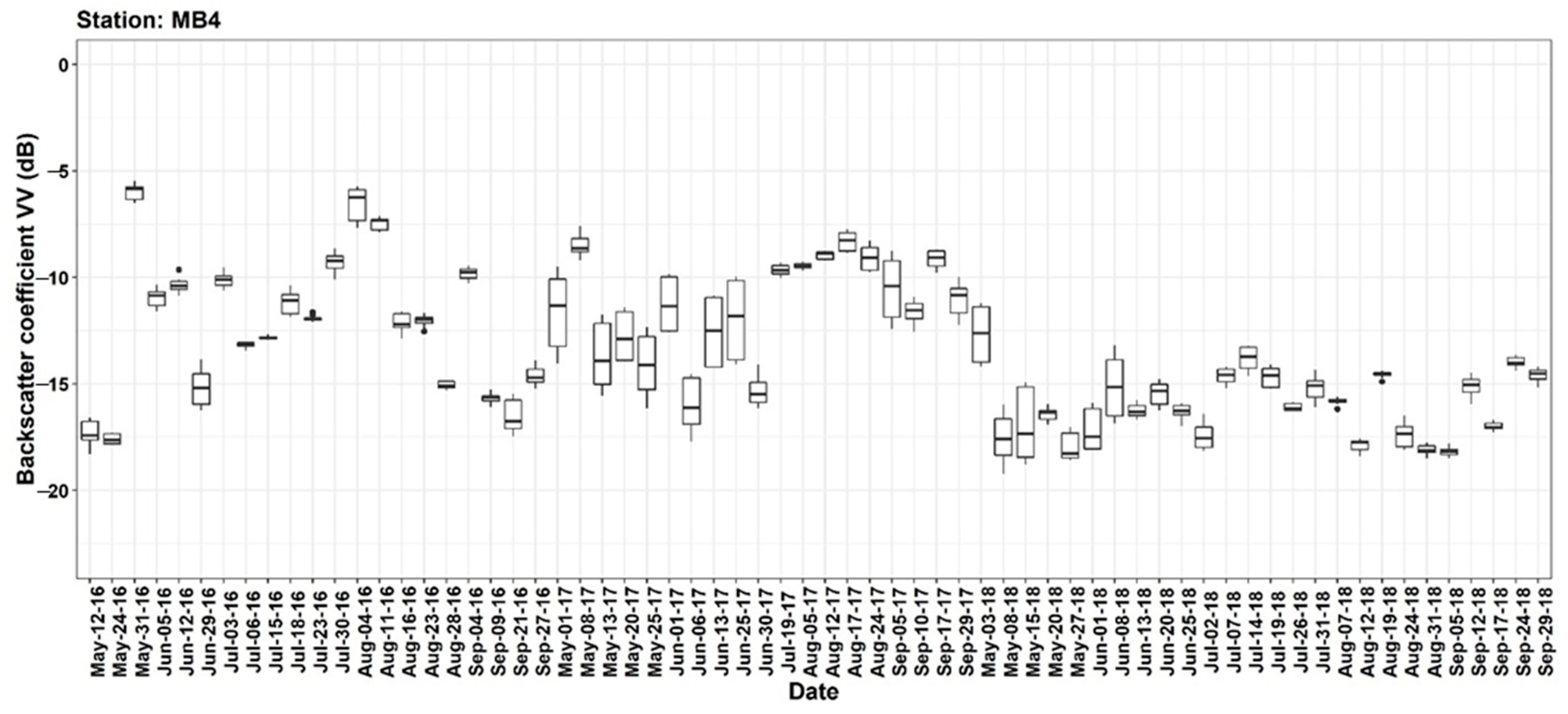
The data period was May to September, corresponding to the crop-growing seasons. We gathered 2016–2018 data from the Agriculture and Agri-Food Canada (AAFC) Real-time In Situ Soil Monitoring for Agriculture (RISMA) network. RISMA collects soil and meteorological information, such as SM, precipitation, air temperature, relative humid, and wind speed, at 15 min intervals and distributes it via their website (https://agriculture.canada.ca/SoilMonitoringStations/ (accessed on 17 January 2020)) [39]. Twelve monitoring stations were located in Manitoba and four in Saskatchewan (Figure 1). SM was measured using three Stevens HydraProbe sensors installed concurrently at depths of 0–5, 5, 20, 50, and 100 cm. In this study, SM data at a depth of 0–5 cm were used to consider the characteristics of the C-band SAR, which finds it difficult to penetrate deep into the ground [40]. These data are defined as calibrated SM, calculated based on the recorded real dielectric permittivity at 0–5 cm (vertical surface sensor), and the unit of SM is m3/m3 [39]. The in situ SM data were adjusted using the calibration equations based on the relationships with the actual dielectric constant derived from the HydraProbe sensors for each site [39,41]. The SM values measured by the three sensors at the same soil depth were usually similar, but occasionally showed significant differences. Therefore, we used the average value when the standard deviation of the three SM values was less than 0.0224 m3/m3. Moreover, only in situ SM data when the rainfall amount was 0 mm were used for SM modeling, because a moisture layer formed on the ground by precipitation or irrigation reduces the backscatter value [42]. The soil texture at the observation stations consisted of sand, sandy loam, loam, silt loam, silty clay loam, clay loam, clay, and heavy clay (Table 2). Among the 12 observation stations in Manitoba, the in situ data from stations MB6, MB8, MB10 (which had heavy clay), and MB4 (which had sandy soil) were not used due to their drainage characteristics. Heavy clay is a low-permeability soil that retains high SM, so a surface moisture layer may readily form via external water inflow [43]. The backscatter measured from heavy clay soil is likely to contain relatively more noise due to the water layer. MB4 was composed of well-drained sand as opposed to heavy clay soil, and exhibited large differences in backscatter between pixels within a 3 × 3 window centered near the station (Figure 2). Such variability can weaken the relationship between the pixel values and in-situ SM when the satellite data are resampled in a coarser window. Based on the 2016 AAFC crop inventory digital map with a resolution of 30 m, most observation data were obtained from the cropland for soybean, barley, canola, spring wheat, and corn. Additionally, parts of the measurements were obtained from grassland and pasture (Table 2). The stations MB3 and MB8 were located close to the roads and were excluded from the analysis.

2.2. Satellite Datasets

S1 consisted of Sentinel-1A and Sentinel-1B, each equipped with a C-band (5.404 GHz) SAR. In this study, we used the Level-1 Ground Range Detected (GRD) product, acquired in the interferometric wide (IW) swath mode. The IW mode is intended for land observations and provides dual-polarization images (VV and VH polarizations). The GRD product uses the WGS84 Earth ellipsoid model with square pixels. The revisitation period for a single S1 is 12 days, and six days for dual S1. The S1 data were preprocessed using the Sentinel Application Platform (SNAP), officially provided by ESA for Sentinel data processing, and the processes included orbit correction, noise removal, radiometric calibration, terrain correction, and unit conversion. Orbit correction was performed to update the precise position and velocity of the satellite because the metadata of the S1 GRD product do not contain accurate information about the orbit. Thermal noise and speckle were removed, as they degraded the quality of the SAR images. Such noise complicates the qualitative or quantitative analysis of SAR images [44,45]. Radiometric calibration was conducted to convert digital pixel values into backscatter values. A terrain correction was conducted to correct the geometric distortion included in the SAR images, which made the SAR image as close to reality as possible using the Shuttle Radar Topography Mission (SRTM) 30 m Digital Elevation Model (DEM). The unit conversion refers to the conversion of the backscatter coefficient (σ°) into decibels (dB), which was conducted using the formula 10 × log10σ°. The angle of incidence in the study area mostly appeared in the ranges 30–37° and 38–40°. As the sensitivity of backscatter to SM is high at low incident angles [46,47] and VV-polarized backscatter tends to be more sensitive to SM than VH-polarized backscatter [47], we used VV-polarized backscatter data with incidence angles less than 37°.
S2 consisted of Sentinel-2A and Sentinel-2B, both equipped with a multispectral instrument and providing 13 bands of multi-spectral data. The revisitation period for a single S2 was 5 days, and the revisiting period for dual S2, which uses two satellites, was 2–3 days. In this study, we used the S2 Level-1C product with a geometric correction, but it required additional atmospheric correction. The atmospheric correction was performed using Sen2Cor in SNAP. SNAP performs an atmospheric correction and classifies the image (e.g., cloud, shadow, vegetation, and water) to generate a Level-2A product. During Sen2Cor processing, the spatial resolution of all data was resampled to 10 m, and the band data except Band 1 (0.443 μm), Band 9 (0.945 μm), and Band 10 (1.375 μm), which have spatial resolutions of 60 m, were automatically converted to Level-2A product. The Level-2A product included data regarding quality-cloud-confidence, quality-snow-confidence, and quality-scene-classification, and provided classification and quality information for each pixel. Quality-cloud-confidence and quality-snow-confidence provide cloud and snow confidence in percentage (%) units, respectively. Quality-scene-classification includes categories such as no data, shadows, vegetation, bare soil, water, clouds, and snow, and the pixel values are integers from 0 to 11. In this study, we used these data to exclude clouds and snow and used only pixel values that referred to bare soil or vegetation. Most cropland pixels were classified as bare soil during May–September and as vegetation during June–August. Five vegetation indices, including NDVI, EVI, the soil- adjusted vegetation index (SAVI), the moisture stress index (MSI), and NDWI, as well as the multispectral bands were used to represent the ground and vegetation conditions (Table 3). Healthy plants absorb red reflectance and reflect near-infrared reflectance. NDVI represents the reflectance characteristics of healthy plants and has a value between −1 and 1, through the normalization of both red and near-infrared reflectance. The closer the value is to 0, the more it corresponds to bare soil, and the closer the value is to 1, the more it corresponds to a higher vegetation vitality [48]. EVI is an index that improves NDVI by additionally using blue reflectance to compensate for the effects of the atmosphere and soil and is designed to be sensitive in areas with high vegetation density [49]. The canopy adjustment factor (L) in the EVI formula is 1, the aerosol correction factors (C1 and C2) are 6 and 7.5, and the gain factor (G) is 2.5 [49]. SAVI is an NDVI index that includes the canopy brightness correction factor (L) to correct for the effect of soil on red and NIR in areas of low vegetation [50]; the L is 0.428 [51]. MSI is an index that measures water stress in plants and is calculated as the ratio of the SWIR to the NIR [52]. SWIR is sensitive to leaf moisture content, and its absorption increases as the leaf moisture content increases [53]. In contrast, NIR is barely affected by changes in the leaf moisture content [54]. NDWI is an index that uses SWIR absorption characteristics for leaf moisture content values that are similar to the MSI [55]. As it is calculated by normalizing NIR and SWIR, its value ranges from −1 to 1; a higher moisture content is indicated by values closer to 1. Band 11 (1.610 μm) data of S2 were used as the SWIR data required to calculate MSI and NDWI.
The 2016 AAFC crop inventory digital map, based on satellite imagery (Landsat-8, Sentinel-2, Gaofen-1, and RADARSAT-2), was used for crop information and to classify the croplands at the in situ stations. It was provided as a GeoTIFF file, and the spatial resolution of the map was 30 m. In this study, the resolution of all satellite data was converted to 30 m to match the spatial resolution of the crop map and to mitigate backscattering noise. Moreover, all the selected image data were transformed into the world geodetic system 1984 (WGS84) and cropped to match the observation data and to produce soil moisture maps.

2.3. Construction of a Comprehensive Dataset for Soil Moisture Modeling

Figure 3 presents a flowchart of the proposed SM model. It is divided into two parts: the construction of the matchup data and the modeling process, the latter of which is discussed in the DNN Modeling Section. The input data for model training consisted of S1 factors (the VV-polarized backscatter coefficient, incidence angle, and elevation), S2 band factors (bands 2–8, band 8A, band 11, and band 12), vegetation indices (NDVI, EVI, SAVI, MSI, and NDWI), crop type, and month. These data were extracted from preprocessed satellite data (S1, S2, and the 2016 AAFC crop inventory digital map) and preprocessed RISMA in situ SM data (Figure 3a). The RISMA in situ data were provided at 15 min intervals. S1 factors, including backscatter data, which are sensitive to changes in SM, were matched with the value closest to the observed time; the maximum time difference was 15 min. The S2 bands and vegetation indices were used to represent the state of the land surface and vegetation, and the time difference between the S2 and S1 data was set to be within 10 days. If any of the matched data were missing, the data for that date were removed. As a result of the filtering, the data of 11 in situ stations (MB1, MB2, MB5, MB7, MB9, MB11, MB12, SK1, SK2, SK3, and SK4) were used for SM estimation modeling. Ultimately, the matchup data consisted of a total of 119 data points collected between May and September from 2016 to 2018.
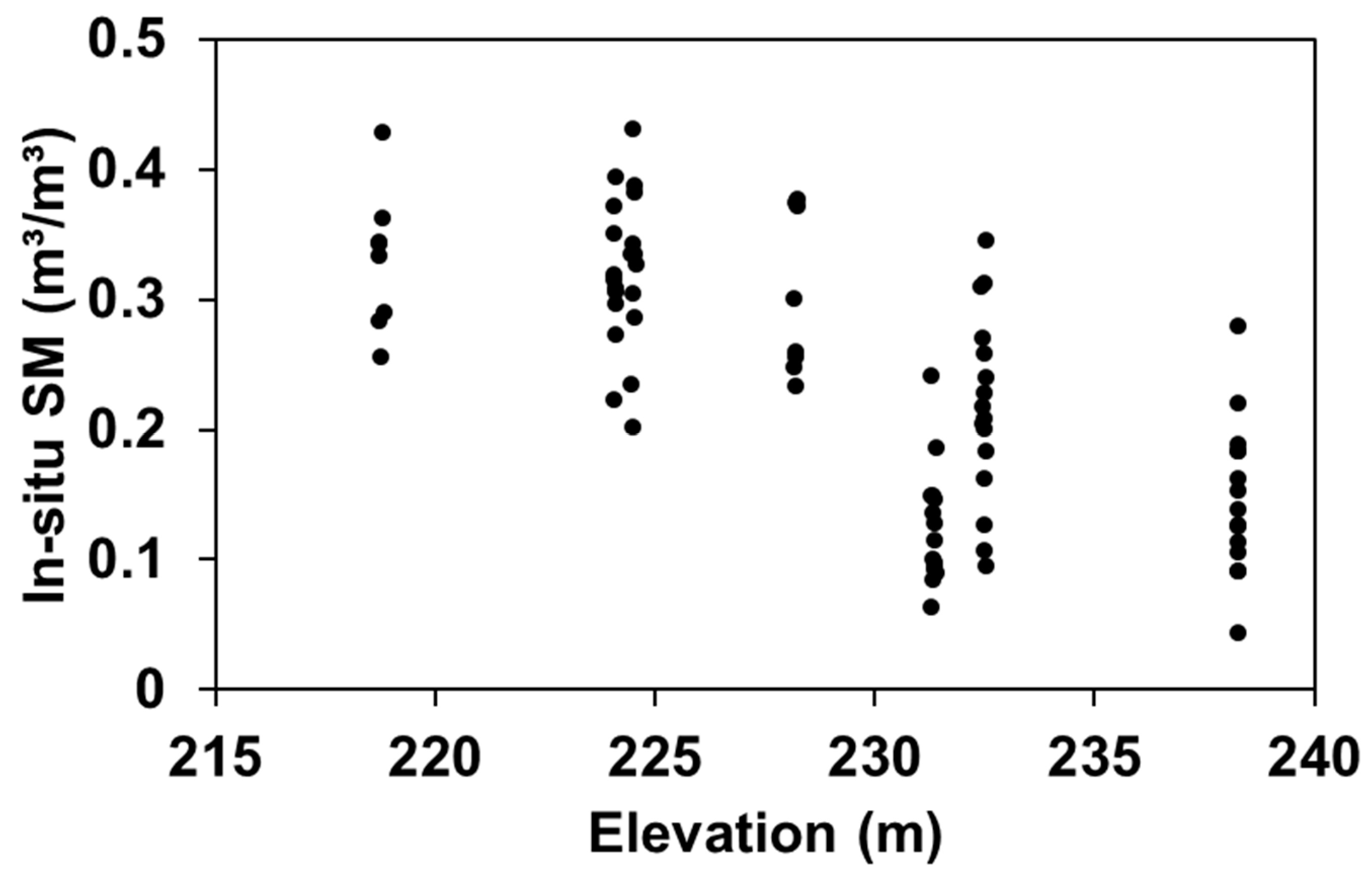
Backscatter typically has a linear relationship with SM [23]. Because backscatter is affected by factors such as the incidence angle, the state of the ground (bare soil or vegetation), crop type, and roughness, these factors should be considered when estimating SM. We used these factors as input data for the SM estimation model. The incidence angle affects the sensitivity of backscatter to the surface roughness, with a lower sensitivity at lower incidence angles than higher ones [56]. Moreover, the sensitivity of backscattering to SM is higher at lower incidence angles [46,47]. Therefore, VV polarization backscatter data with incidence angles less than 37° were used for accurate SM estimation. Elevation derived from DEM is a variable that can affect the distribution of SM. SM can be relatively low at higher elevations, as water moves from higher to lower places due to gravity [57,58]. This characteristic was found in Manitoba, where SM showed a slight decreasing trend according to elevation (Figure 4). RMSH and correlation length (CL) are also used as topographical factors that affect water distribution. We evaluated the variable importance for the three variables (elevation, RMSH, and CL), and Appendix A shows that elevation was an appropriate variable for SM modeling. Moreover, a standardized dataset for elevation, such as SRTM, is available globally. Vegetation generally causes volumetric scattering and weakens the backscatter reflected by the soil [59], thus affecting the SM estimate using backscattering. The S2 multi-spectral bands and vegetation indices were used to reflect the vegetation state and water stress. The S2 multi-spectral bands after atmospheric correction using Sen2Cor consisted of blue (band 2), green (band 3), red (band 4), red edge (bands 5–7), NIR (bands 8 and 8A), and SWIR (bands 11 and 12). Blue, green, red, and NIR are useful bands with which to analyze the characteristics of vegetation and soil and are used to calculate vegetation indices, such as NDVI, EVI, and SAVI; they are also used for land cover classification [60]. The red edge was designed for vegetation analysis and is used as a descriptor of the chlorophyll content [61]. SWIR is sensitive to ground moisture content and is used for plant water stress assessments and snow/ice/cloud classification [62]. SWIR and NIR are used to calculate MSI and NDWI, which indicate plant water stress (Table 3). Depending on the crop, differences in canopy structure and roughness affect the sensitivity of backscatter to SM [63,64]. Therefore, crop type was selected as an input variable and was used in numerical form (Table 4). In addition, the structure of crops can be divided according to the phenological stages, which are typically distinguished on a monthly basis [65]. Thus, monthly information was used as an input variable, because it can be used to classify the condition of structurally similar crops.

2.4. DNN Modeling

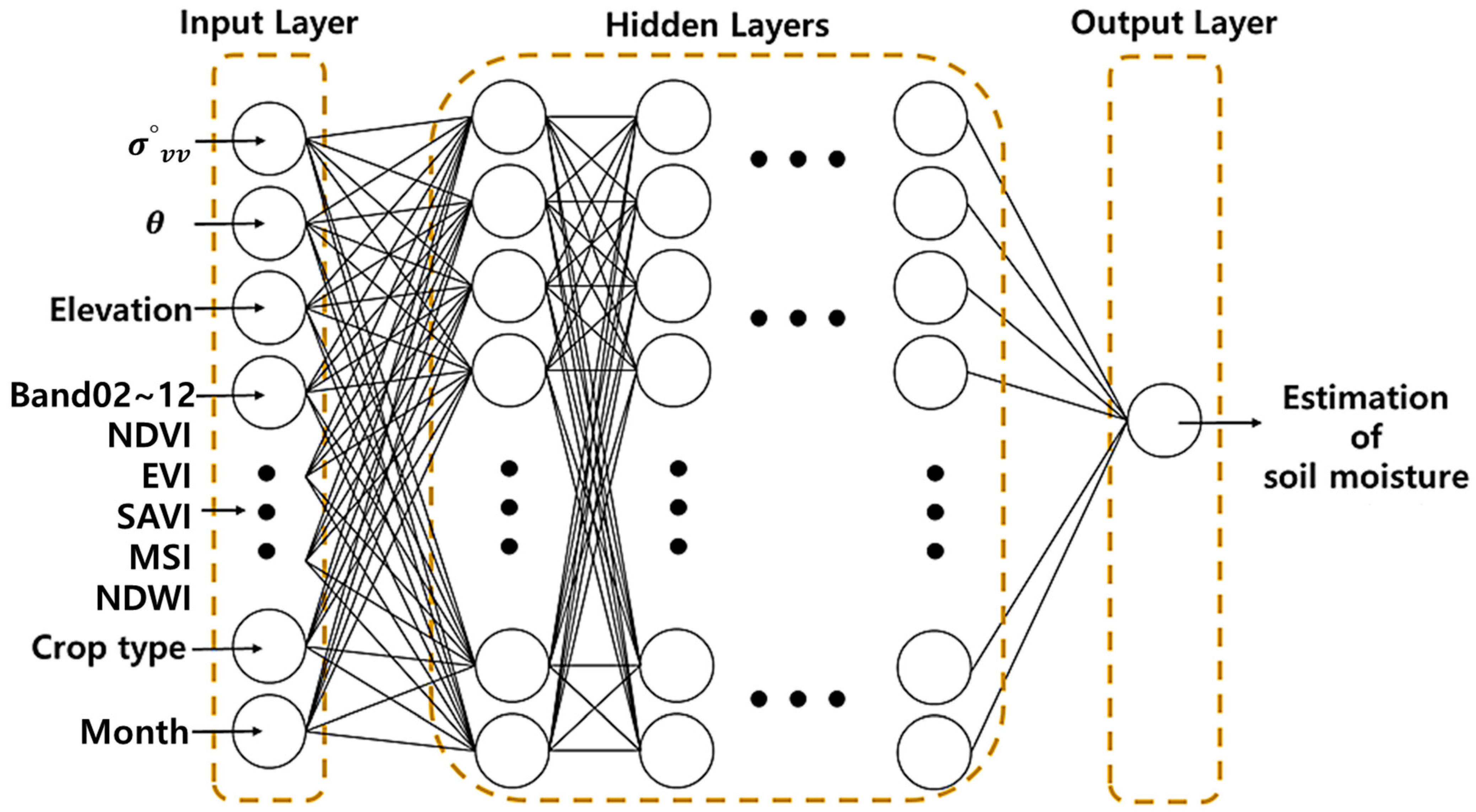
We used the H2O package to build a deep learning model for SM estimation. H2O is a Java-based open-source ML platform. The DNN model consisted of an input layer, hidden layers, and an output layer (Figure 5). The input layer consisted of 20 nodes receiving S1 factors (VV polarized backscatter coefficient, incidence angle, and elevation), S2 band factors (bands 2–8, band 8A, band 11, and band 12), vegetation indices (NDVI, EVI, SAVI, MSI, and NDWI), crop type, and month. The output layer consisted of a single node to estimate SM. We used default values for most of the model hyperparameters and changed four hyperparameters (hidden layer (H), node (N), dropout ratio (DR), and epoch (E)). The main hyperparameters of H2O deep learning that were set to default values were: activation function = ‘RectifierWithDropout’, L1 regularization = 0, L2 regularization = 0, and optimizer = ‘AdaDelta’. RectifierWithDropout refers to ReLU with a dropout ratio applied. ReLU is a function that returns the input value, as is, if it exceeds 0, and returns 0 if the value is less than 0 [66]. This prevents the vanishing gradient problem, which is a learning interruption problem that occurs during the backpropagation process due to the sigmoid function used in traditional ML [66]. The dropout ratio is a technique used to remove some nodes to avoid overfitting (which is a problem encountered with DNN) [67] and is implemented at each layer in the neural network. Overfitting means that, while the training error is small due to overtraining on the training data, the error is large on the validation data. For example, a dropout ratio = 0.2 means that 20% of the nodes existing in the layer are excluded from training. L1 and L2 regularization, along with the dropout ratio, are parameters used to reduce model complexity and prevent overfitting [68]. L1 regularization is a method to limit the absolute value of weights, and L2 regularization is a method to limit the sum of squared weights [68]. Adaptive delta (AdaDelta) is an optimizer used to minimize the loss function and improve learning speed. It is a technique that improves the Adagrad problem, in which the learning rate approaches zero as training progresses, resulting in ineffective learning [69].
In this study, to find the optimal estimate model for SM, models were constructed and evaluated under various hyperparameter conditions: hidden layer (H: 3–4), node (N: 100–400, interval: 100), epoch (E: 1–200, interval: 5), and dropout ratio (DR: 0.05–0.25, interval: 0.05) (Figure 3b). Each model was trained and evaluated using the k-fold cross-validation (CV) (k = 10). This method randomly divides the entire dataset into k sets and performs k evaluations. During the k evaluations, (k − 1) sets are used as training data, and the remaining set is used as the validation set. The validation set is not duplicated and changes with each iteration. As this method uses all datasets for training and evaluation, more generalized models can be built. In this study, we adopted this method to mitigate the potential overfitting that can occur when a small number of matchup data are divided into training and validation datasets. The matchup data, composed of 119 data points gathered between May and September from 2016 to 2018, were randomly divided into ten sets. Each set was then utilized for conducting ten-fold CV experiments for each model. The accuracy of the models was evaluated quantitatively using mean bias error (MBE), mean absolute error (MAE), RMSE, and CC. In addition, for an objective evaluation of the model performance, an accuracy comparison was performed using top layer SM data (0–5 cm), derived from SMAP L4 Global 3 hourly 9 km EASE-Grid Surface and Root Zone Soil Moisture Geophysical Data. SMAP SM data were extracted based on values close to in situ data in terms of space and time, and their accuracy compared with in situ data was calculated.

3. Results and Discussion

3.1. Model Accuracy and Optimal Model

To find the optimal DNN model for estimating SM, we constructed various models by changing the values of four hyperparameters (hidden layer, node, dropout ratio, and epoch) and evaluated these models through the ten-fold CV. Table 5 summarizes the RMSE and CC of each model based on the low RMSE for an objective evaluation. In Table 5, Model 1 (H = 4, N = 300, DR = 0.1, E = 200) had the greatest accuracy (RMSE = 0.0416 m3/m3, CC = 0.9226). Table 6 presents the CV results for each fold of Model 1. The average MBE of Model 1 was 0.0042 m3/m3, which was close to the 0 bias, and the average MAE was 0.0315 m3/m3. The average CC was 0.9226, suggesting a strong linear relationship between the estimated and observed SMs. The accuracy and correlation showed a much higher performance than the 9 km SMAP SM data (Figure 6). The proposed Model 1’s estimates were more densely clustered along the 1:1 line than the points representing SMAP data in the scatterplot between the estimated and observed values (Figure 6). In other words, the estimated SM values from the proposed model were more consistent with the observed values than the SMAP data. Among the ten CVs of Model 1, CV4 and CV8 presented RMSE values of 0.0585 m3/m3 and 0.0522 m3/m3 respectively, which were higher than the average RMSE, but maintained a high positive CC (Table 6). This was judged to be less accurate for some CVs, because a ten-fold CV was performed with 119 small matchup data.
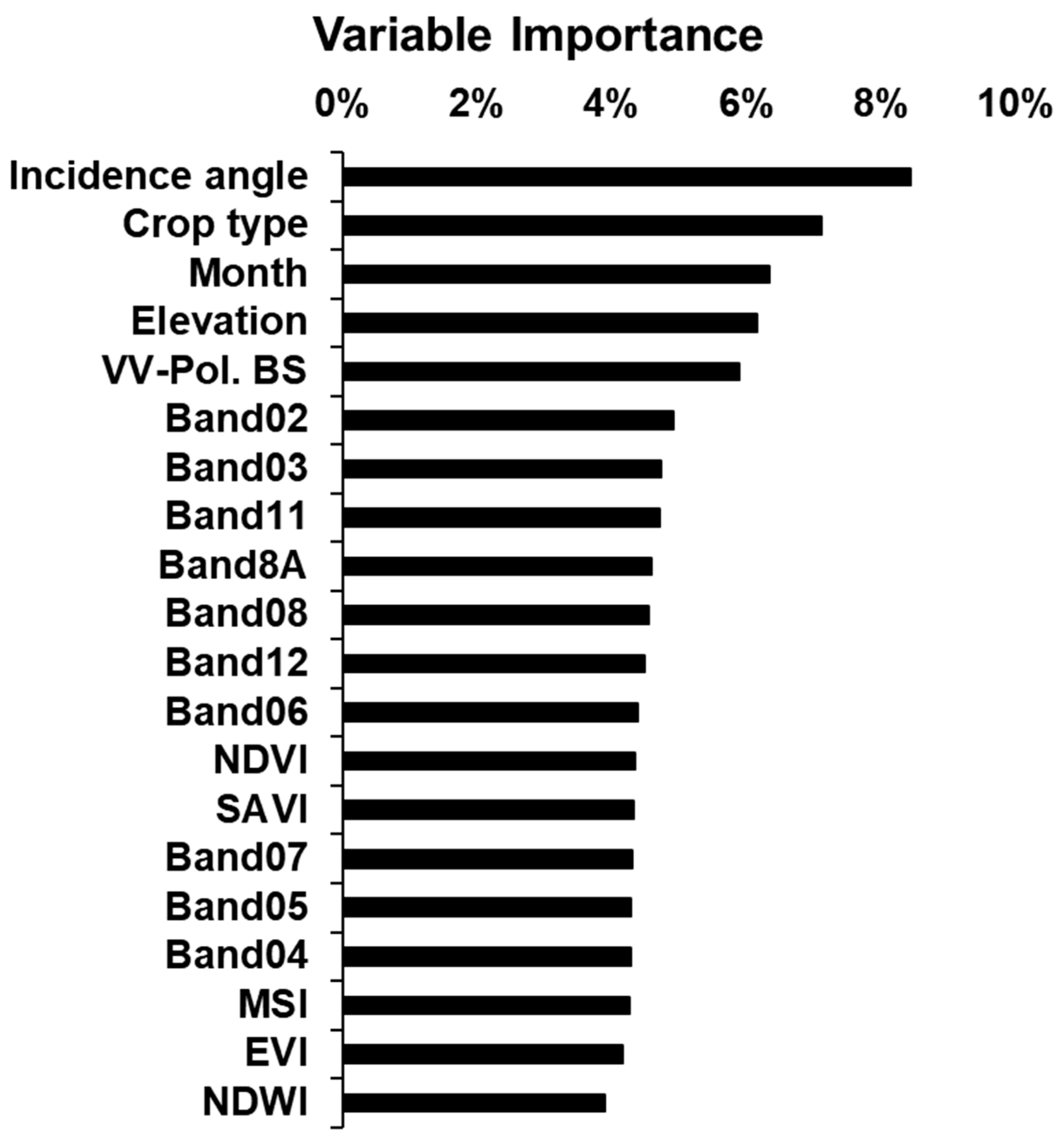
The H2O library used for DNN modeling provides the importance of input variables calculated through the Gedeon method. This method calculates their importance by considering the weights connecting the input features to the first two hidden layers, and the derived importance represents the significance of the variables for the prediction outcome as a percentage [70,71]. Among the input variables, the incident angle, crop type, month, elevation, and backscattering showed an importance of about 6% or more, while the bands and vegetation indices related to S2 showed an importance of about 4% (Figure 7). Particularly, the incident angle, crop type, month, and elevation used to reflect the sensor and ground conditions that affect backscattering in the model showed higher importance in predicting SM than backscattering, which has a direct relationship with SM (Figure 7). This means that including the sensor and local factors that affect backscatter helps to achieve more accurate SM estimates when modeling for SM across several study areas.
For a more accurate SM estimate, we used data only when precipitation was 0 mm. However, even if there was no precipitation at a certain time, precipitation that may have fallen in the past might affect backscattering by forming a water layer on the ground (standing water), or changing SM or ground roughness. Therefore, we calculated the sum of the rainfall that occurred in the 24 h before the time of the observation data and investigated the effect of daily rainfall intensity on the accuracy of SM. The accuracy was high on non-rainy days and low on rainy days (Table 7). Specifically (Table 8), when the daily precipitation was ≤5 mm/day, the accuracy was similar to that when the daily precipitation was 0, whereas when the daily precipitation was >5 mm/day, the RMSE and MAE increased to 0.0656 m3/m3 and 0.0531 m3/m3, respectively, and showed a tendency to underestimate SM (MBE = −0.0185 m3/m3). Precipitation contributes to surface erosion, saturation of SM, and the formation of standing water [43,72,73]. Moreover, surface scattering occurs more in wet vegetation after rainfall than volume scattering does [74]. As a result, backscatter tends to decrease under these conditions, suggesting that SM is underestimated due to high precipitation.
The accuracy of SM was the best within the NDVI range of 0.3 < NDVI ≤ 0.7, which corresponded to the vegetation growth stage, and was low when the vitality of vegetation was high (NDVI > 0.7) or low (NDVI ≤ 0.3) (Table 9). High vegetation vitality corresponds to a period of maximum crop growth [75]. During this time, the soil is likely to be in a state of “dense vegetation” and completely covered by the vegetation canopy [75]. Vegetation serves to attenuate microwave signals reflected from the soil [59]. Therefore, the accuracy was low at a higher NDVI due to this effect (RMSE = 0.0524 m3/m3, CC = 0.8662). The accuracy of SM at NDVI ≤ 0.3, which is close to bare soil, was affected by precipitation. In the case of no rain, the accuracy of SM was similar to the condition in which the NDVI was >0.3 and ≤0.7, but MAE, RMSE, and CC significantly deteriorated in the rain (Table 9 and Table 10).
Taken together, the presence of fully grown vegetation and precipitation are factors that can cause an inaccurate SM estimation. However, the CCs were generally higher than about 0.9 and the CC was 0.7249–0.9049 in cases of precipitation or heavy vegetation (Table 7, Table 8, Table 9 and Table 10). This means that, although accuracy may decrease due to precipitation and vegetation, the estimated SM based on the DNN was strongly positively correlated with the observed SM.
To determine the effect of meteorological factors (daily precipitation, air temperature, and relative humidity) on SM, the correlation between meteorological factors for each station and estimated SM was analyzed. As with precipitation data, air temperature and relative humidity also used the average relative humidity (%) and average air temperature data (°C) provided by RISMA. When calculating the correlation, any instances missing at least one weather variable were excluded. SM was positively correlated with precipitation (CC = 0.3781–0.7362) at all stations except SK3 (Table 11). Air temperature and relative humidity are factors that affect evaporation, which causes a loss of SM. SM showed a negative correlation with air temperature and a positive correlation with relative humidity. However, there were some differences in variables affecting SM for each station. In MB1, MB7, MB9, MB11, and MB12, SM showed a higher correlation with relative humidity than air temperature (Table 11). On the other hand, SM in MB2, MB5, SK3, and SK4 showed a higher correlation with temperature than relative humidity (Table 11). In general, evapotranspiration tends to increase with higher temperatures, but this is limited by humidity [76]. Because of this, the effect will have been different at each station. However, a very weak correlation with precipitation was confirmed at station SK3 (CC = 0.1920), and almost no correlation was found between air temperature and relative humidity at stations SK1 and SK2 (Table 11). This is presumed to be attributable to yet unclear factors affecting SM, such as irrigation. In addition, it was confirmed that the relationship between SM and meteorological variables had a complex and nonlinear structure rather than a simple linear relationship. This re-emphasizes that DNN-based modeling that effectively reflects the complexity and nonlinearity of various variables is essential for SM modeling. One of the most considerable limitations of current SM modeling is the absence of high-resolution meteorological factor data and data related to irrigation. If these data can be made available in the future, the accuracy of high-resolution SM modeling will be greatly improved.

3.2. Soil Moisture Mapping at the Local Scale

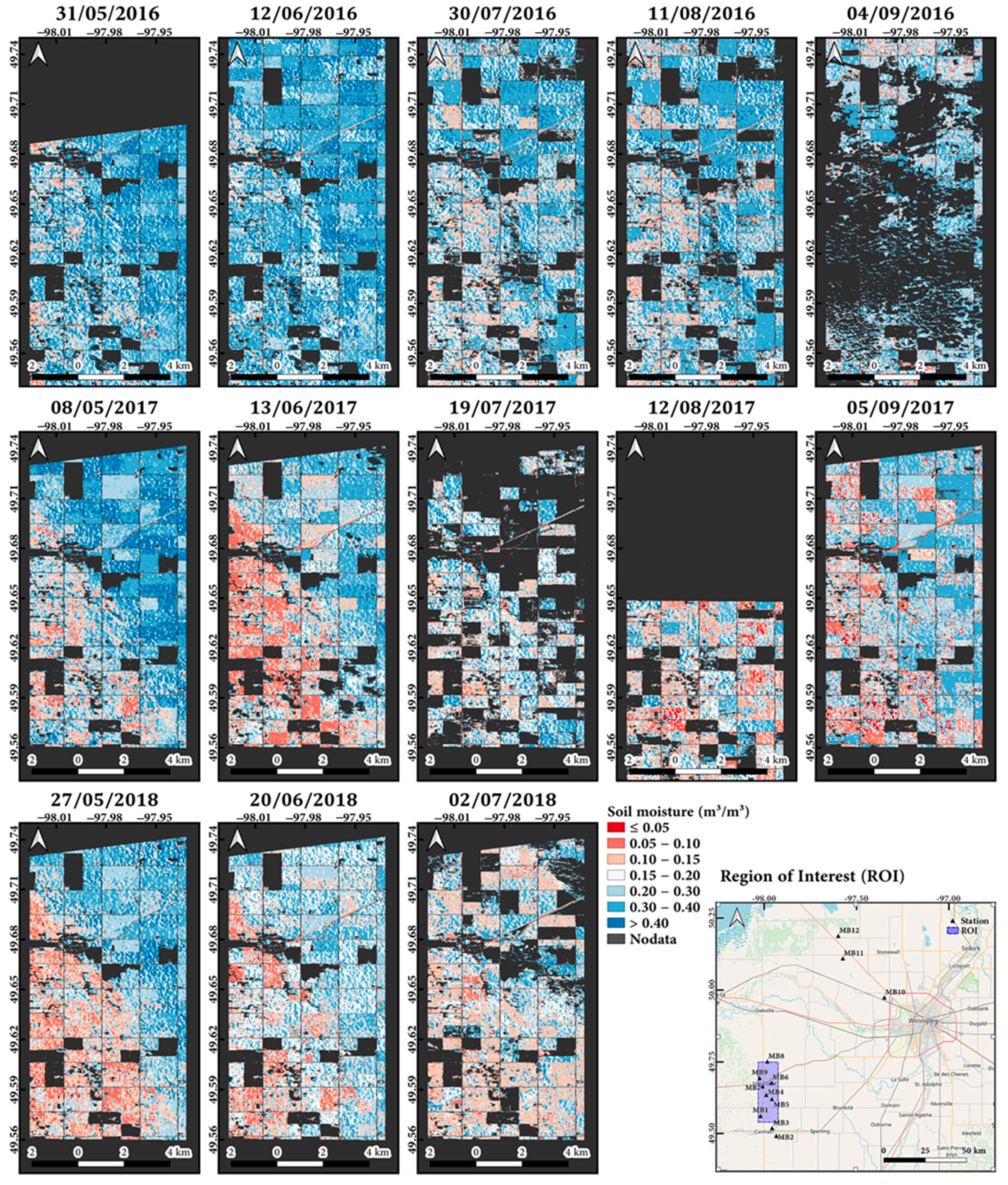
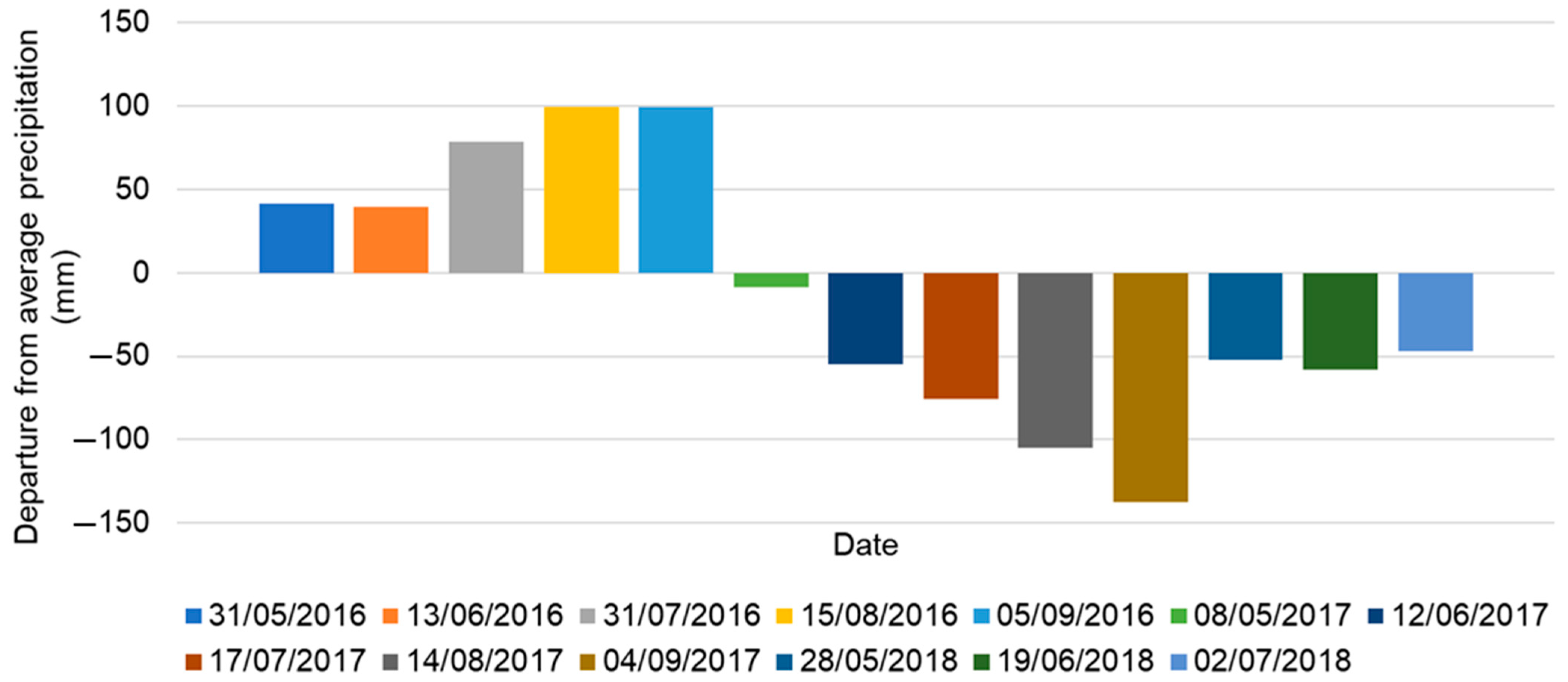
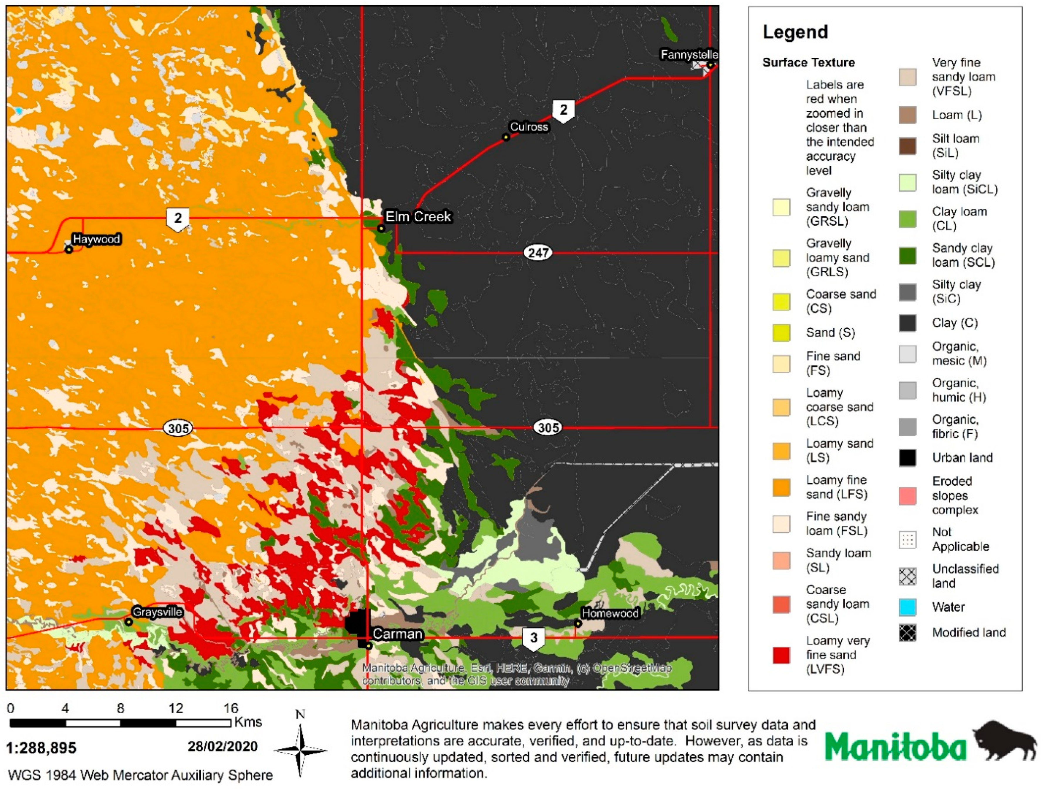
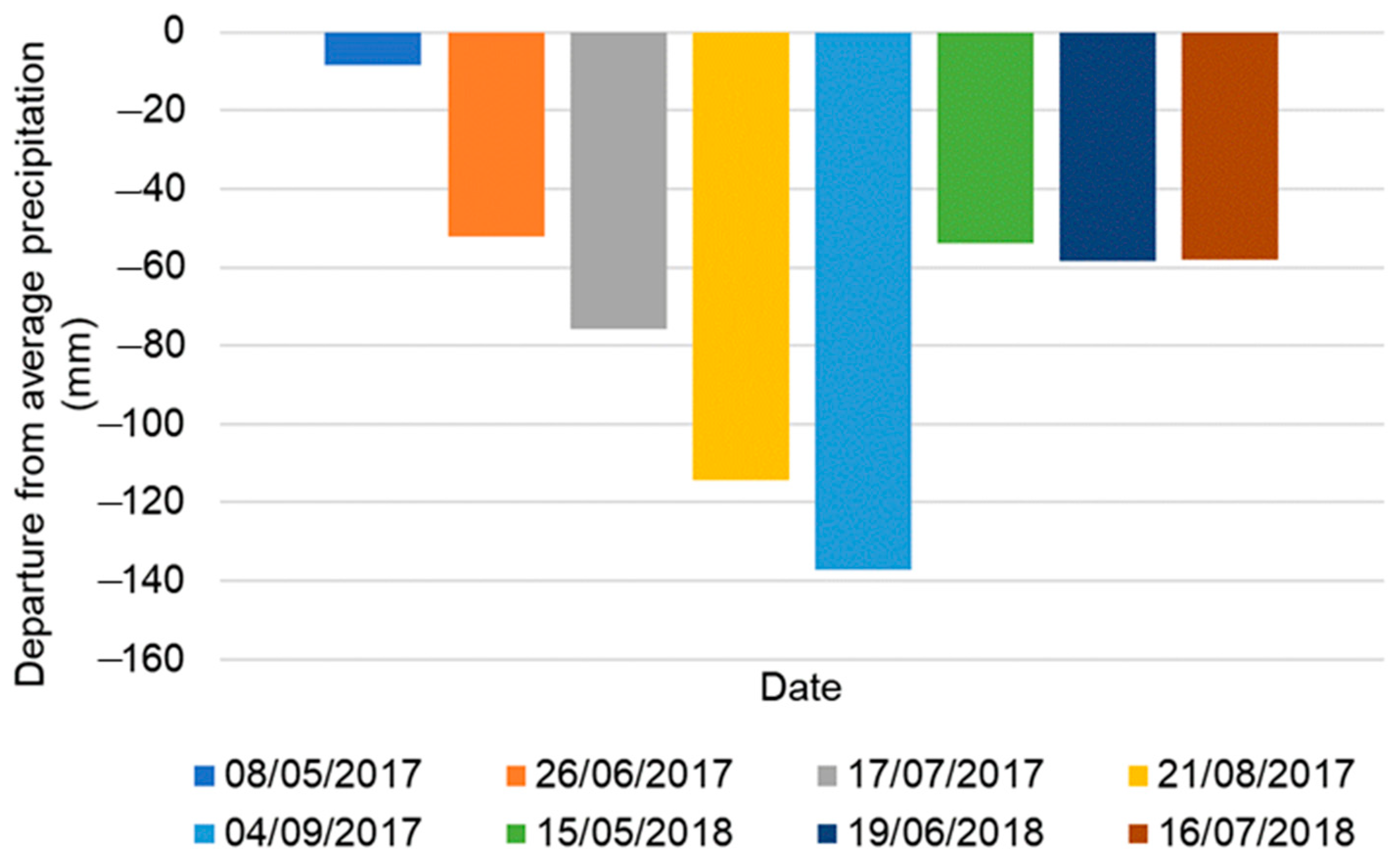
Figure 8 and Figure 9 present SM maps for the Carman and Sturgeon Creek watersheds in Manitoba, respectively. Pixels that did not match the conditions of the input data used in the DNN model (e.g., crop type, no data, shadows, water, clouds, and snow) were excluded from the SM estimate and are represented by a gray color, which indicates that there are no data on the map (Figure 8 and Figure 9). Some areas were not represented in the SM maps. We used the departure from average precipitation (DAP) (mm) data provided by the Government of Canada to compare SM. DAP was defined as the accumulated precipitation value from the beginning of growing season, specifically from 1 April, subtracted from the long-term average value. The long-term average precipitation was defined as the average amount during 1981–2010 [77]. A negative DAP value indicates less than average precipitation, while a positive DAP value indicates above-average precipitation [77]. To facilitate this comparison, we compared SM maps with the DAP data of the closest date to the SM maps. SM in the two regions was related to precipitation. In particular, the Carman region had a relatively low SM distribution from May 2017 to July 2018 (Figure 8). This was consistent with the decrease in precipitation (DAP < 0) in 2017 and 2018 compared to 2016 (Figure 10). However, the area northeast of Carman showed no significant change in SM compared to the southwest (Figure 8). This distribution of SM was closely related to the soil texture. In this area, sandy and loam-based soils exist in the southwest, while clay-based soils are in the northeast (Figure 11). Clay-based soils have small soil particles that do not drain well [39,78]; thus, their SM was generally high regardless of the season (Figure 8).
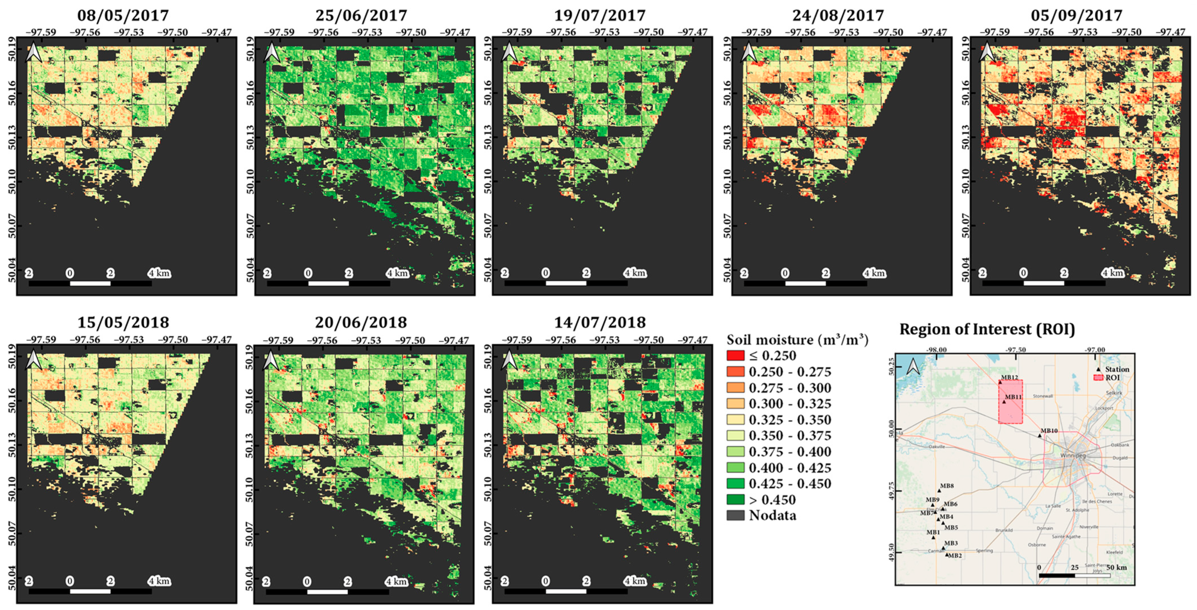
The Sturgeon Creek watershed is located northwest of Winnipeg, Manitoba, Canada. The region of interest (ROI) shown in Figure 9 corresponds to the downstream region of the Sturgeon Creek watershed [78]. Although DAP in this area was generally negative, SM was consistently distributed over 0.20 m3/m3 regardless of the season (Figure 9 and Figure 12). This was also related to the soil texture. The soil in this area is clay, which does not drain well [78]. Bhuiyan et al. (2017) [78] reported that SM was generally distributed over 0.20 m3/m3 in the October 2014 SM map for this area. However, notably, slightly reduced SM distributions were observed on 24 August 2017 and 5 September 2017, close to 21 August 2017 and 4 September 2017, when DAP was below −80 mm (Figure 9 and Figure 12). This means that, even if the soil is composed of clay, the SM can decrease under fairly low precipitation. Overall, clay retains more SM than other soil types. Although soil texture information was not included as input data in the model, the mapping results show that the estimated SM fairly reflected local and seasonal characteristics. Therefore, it is expected that using soil texture information as input data will lead to more accurate modeling.

4. Conclusions

In this study, we conducted DNN-based SM modeling for croplands in Manitoba and Saskatchewan, Canada, using high-resolution image data (e.g., S1 SAR, S2 multi-spectral data, and AAFC crop maps) with resolutions ranging from 10 to 60 m to estimate SM at a regional scale. The model was built through hyperparameter optimization, and its accuracy was evaluated according to daily precipitation and vegetative growth. The model had an RMSE of 0.0416 m3/m3 and a CC of 0.9226. The SM values estimated from the proposed model were in better agreement with the in situ values than the SMAP data. The accuracy tended to be higher when daily precipitation was zero or very low, as opposed to when it was higher (RMSE = 0.0333–0.0374 m3/m3 and CC = 0.9211–0.9417 m3/m3). This is because precipitation can affect backscattering by contributing to surface erosion, saturation of SM, and the formation of standing water [43,72,73]. Additionally, the accuracy improved during periods of bare soil and vegetative growth (0 < NDVI ≤ 0.7). Although the accuracy decreased during high precipitation and the presence of vegetation with high NDVI, the estimated SM remained strongly correlated with the observed SM (CC = 0.7249–0.9049). Furthermore, we confirmed from the SM maps that the estimated SM generally reflected the regional soil characteristics, even if the soil texture information was not used as an input variable.
One of the most considerable limitations of high-resolution SM modeling is the current lack of high-resolution data on weather and irrigation. Meteorological factors can affect the increase in and loss of SM, but this study confirmed that the relationship between SM and weather variables (precipitation, temperature, and relative humidity) is not just a linear relationship, but a complex and nonlinear relationship. Moreover, some results showing a weak correlation of less than 0.4 between the predicted SM and meteorological factors suggest that yet unclear factors, such as irrigation, are affecting SM. Irrigation is the process of artificially supplying water to crops when the natural water supply is not sufficient for plant growth, and it affects SM through different ways, such as soil salinity, soil temperature, runoff, and erosion. First, proper irrigation during crop growth prompts an increase in SM, thereby relieving water stress in plants and improving crop growth and yields [80,81,82,83,84]. Second, irrigation with low- or medium-salinity water reduces soil salinity via leaching [85], and hence it affects SM by promoting root water absorption by plants [86,87]. On the other hand, in soils with high salinity, the ability of plants to absorb water diminishes [86,87]. Third, irrigation reduces surface temperatures by increasing evapotranspiration, along with increasing SM [84,88]. It thus helps plants to grow by preventing stress at high temperatures and supplying SM [88,89]. Fourth, excessive irrigation can lead to runoff and erosion [90,91,92]. As this runoff water moves down slopes, it evaporates, leaving less water stored in the soil for plant growth [90]. The erosion changes surface roughness, which influences the backscattering of radar [93]. Thus, irrigation data are crucial for estimating SM, but detailed data for irrigation are not usually available [94]. Therefore, it is essential to secure high-resolution meteorological data and local agricultural data (such as that regarding irrigation) in the future. Additionally, if various data (e.g., SAR/optical images, meteorological images, and local ground data (such as soil texture, roughness, vegetation, and irrigation)) are produced, and SM modeling that integrates these data is performed using DNN (which is effective in dealing with complexity and nonlinearity between variables), more accurate SM estimation across a wider area will be possible.

Author Contributions

Conceptualization, S.-J.L. and Y.L.; methodology, S.-J.L. and Y.L.; formal analysis, S.-J.L.; data curation, S.-J.L.; writing—original draft preparation, S.-J.L. and Y.L.; writing—review and editing, S.-J.L., C.C., J.K., M.C., J.C. and Y.L. All authors have read and agreed to the published version of the manuscript.

Funding

This research was supported by Basic Science Research Program through the National Research Foundation of Korea (NRF) funded by the Ministry of Education (NRF- 2022R1I1A1A01073185). This work was conducted with the support of the “Cooperative Research Program for Agriculture Science & Technology Development (PJ014787042023)”, Rural Development Administration, Republic of Korea.

Conflicts of Interest

The authors declare no conflict of interest.

Abbreviations

AAFCAgriculture and Agri-Food Canada
AdaDeltaAdaptive Delta
CCCorrelation Coefficient
CDChange Detection
CVCross-Validation
dBDecibels
DAPDeparture from Average Precipitation
DEMDigital Elevation Model
DNNDeep Neural Network
DRDropout Ratio
ESAEuropean Space Agency
EVIEnhanced Vegetation Index
GRDGround Range Detected
GRNNGeneralized Regression Neural Network
HHidden Layer
IEMIntegral Equation Model
IFOVInstantaneous Field of View
IWInterferometric Wide
LSTLand Surface Temperature
MAEMean Absolute Error
MBEMean Bias Error
MLMachine Learning
MSIMoisture Stress Index
NASANational Aeronautics and Space Administration
NDMINormalized Differential Moisture Index
NDVINormalized Difference Vegetation Index
NDWINormalized Difference Water Index
NIRNear-Infrared
NNNeural Network
OLSOrdinary Least Squares
ReLURectified Linear Unit
RFRRandom Forest Regression
RISMAReal-Time In Situ Soil Monitoring for Agriculture
RMIRadar Moisture Index
RMSHRoot-Mean-Square Height
RMSERoot-Mean-Square Error
ROIRegion of Interest
RTMRadiative Transfer Model
S1Sentinel-1
S2Sentinel-2
SARSynthetic-Aperture Radar
SAVISoil-Adjusted Vegetation Index
SDStandard Deviation
SMSoil Moisture
SMAPSoil Moisture Active Passive
SMOSSoil Moisture and Ocean Salinity
SNAPSentinel Application Platform
SRTMShuttle Radar Topography Mission
SVMSupport Vector Machine
SVRSupport Vector Regression
SWIRShortwave Infrared
TDRTime-Domain Reflectometry
TVDITemperature Vegetation Dryness Index
VIVegetation Index
VHVertical–Horizontal
VVVertical–Vertical
WCMWater Cloud Model

Appendix A

The importance of topographical variables (elevation, RMSH, and CL) was evaluated to investigate the topographical effect on SM modeling. RMSH was an index to quantify vertical roughness, calculated by Equation (A1) [95]:
RMSH = i = 1 n ( z i z ¯ ) 2 n 1
where n is the number of data points chosen; z i indicates the elevation value of the point i ; and z ¯ is the average elevation of the all the data points. CL is obtained by the autocorrelation function (Equation (A2)) [96,97]:
ρ ( h ) = i = 1 n ( h ) z i z i + h i = 1 n z i 2
where ρ ( h ) indicates the autocorrelation function, which measures the correlation between the elevation at point i (represented as z i ), and the elevation at another point located a distance h away from it (denoted to as z i + h ) [97]. For each distance h, n(h) is the number of pairs taken into account [97]. CL is defined as the distance where the value of ρ ( h ) reaches 1/e [97]. In the study, the CL was calculated using the ‘geodiv’ package for surface roughness in the statistical programming language R. The ‘scl’ function in the package computes the CL using an area autocorrelation function [98].
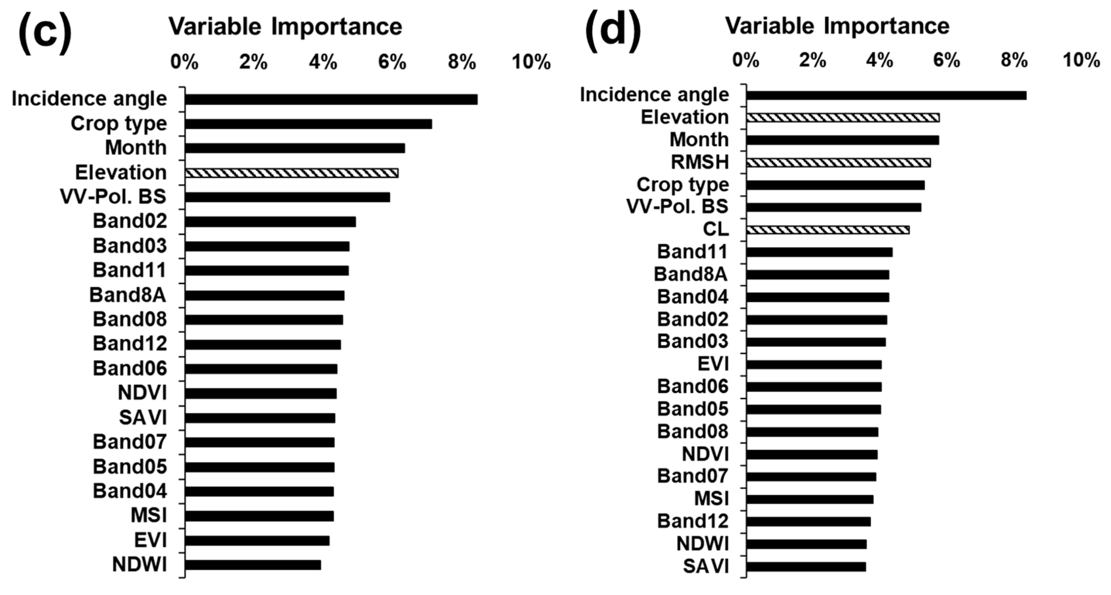
When using each one of the three variables, the variable importance of elevation, RMSH, and CL were 6.14%, 6.12%, and 5.50%, respectively (Figure A1a–c). Additionally, when the variable importance experiment that included all topographic variables was performed, the variable importance of elevation, RMSH, and CL were 5.74%, 5.48%, and 4.85%, respectively (Figure A1d). Thus, we chose elevation as the topographic variable for SM. Additionally, NASA SRTM is a common dataset available for the global values of elevation.
Figure A1. Variable importance according to the use of topographic variables: (a) RMSH, (b) CL, (c) elevation, and (d) all the three variables.
Remotesensing 15 04063 g0a1aRemotesensing 15 04063 g0a1b

References

  1. Robock, A. HYDROLOGY|Soil Moisture. In Encyclopedia of Atmospheric Sciences; Academic Press: Cambridge, MA, USA, 2003; pp. 987–993. [Google Scholar]
  2. Engman, E.T. Soil Moisture: The Hydrologic Interface between Surface and Ground Waters; Laboratory for Hydrospheric Processes Research Publications: Greenbelt, MD, USA, 1997. [Google Scholar]
  3. Al-Yaari, A.; Wigneron, J.P.; Ducharne, A.; Kerr, Y.H.; Wagner, W.; De Lannoy, G.; Mialon, A. Global-Scale Comparison of Passive (SMOS) and Active (ASCAT) Satellite Based Microwave Soil Moisture Retrievals with Soil Moisture Simulations (MERRA-Land). Remote Sens. Environ. 2014, 152, 614–626. [Google Scholar]
  4. Arora, V.K.; Boer, G.J. The Temporal Variability of Soil Moisture and Surface Hydrological Quantities in a Climate Model. J. Clim. 2006, 19, 5875–5888. [Google Scholar] [CrossRef]
  5. Trugman, A.T.; Medvigy, D.; Mankin, J.S.; Anderegg, W.R.L. Soil Moisture Stress as a Major Driver of Carbon Cycle Uncertainty. Geophys. Res. Lett. 2018, 45, 6495–6503. [Google Scholar] [CrossRef]
  6. Verhoest, N.E.; Lievens, H.; Wagner, W.; Álvarez-Mozos, J.; Moran, M.S.; Mattia, F. On the Soil Roughness Parameterization Problem in Soil Moisture Retrieval of Bare Surfaces from Synthetic Aperture Radar. Sensors 2008, 8, 4213–4248. [Google Scholar]
  7. Seneviratne, S.I.; Corti, T.; Davin, E.L.; Hirschi, M.; Jaeger, E.B.; Lehner, I.; Orlowsky, B.; Teuling, A.J. Investigating Soil Moisture—Climate Interactions in a Changing Climate: A Review. Earth-Sci. Rev. 2010, 99, 125–161. [Google Scholar] [CrossRef]
  8. Caldwell, T.G.; Bongiovanni, T.; Cosh, M.H.; Halley, C.; Young, M.H. Field and Laboratory Evaluation of the CS655 Soil Water Content Sensor. Vadose Zone J. 2018, 17, 1–16. [Google Scholar] [CrossRef]
  9. Bittelli, M. Measuring Soil Water Content: A Review. HortTechnology 2011, 21, 293–300. [Google Scholar] [CrossRef]
  10. Lee, C.S.; Sohn, E.; Park, J.D.; Jang, J.D. Estimation of Soil Moisture Using Deep Learning Based on Satellite Data: A Case Study of South Korea. GISci. Remote Sens. 2019, 56, 43–67. [Google Scholar] [CrossRef]
  11. Neelam, M.; Mohanty, B.P. Global Sensitivity Analysis of the Radiative Transfer Model. Water Resour. Res. 2015, 51, 2428–2443. [Google Scholar] [CrossRef]
  12. Bhatta, B. Research Methods in Remote Sensing; SpringerBriefs in Earth Sciences; Springer: Dordrecht, The Netherlands, 2013. [Google Scholar]
  13. Sheffield, J.; Xia, Y.; Luo, L.; Wood, E.F.; Ek, M.; Mitchell, K.E. North American Land Data Assimilation System: A Framework for Merging Model and Satellite Data for Improved Drought Monitoring. Remote Sens. 2012, 4, 1902–1924. [Google Scholar]
  14. European Space Agency (ESA). Sentinel-2 MSI User Guide. Available online: https://sentinels.copernicus.eu/web/sentinel/user-guides/sentinel-2-msi (accessed on 1 May 2023).
  15. Das, K.; Paul, P.K. Present Status of Soil Moisture Estimation by Microwave Remote Sensing. Cogent Geosci. 2015, 1, 1084669. [Google Scholar] [CrossRef]
  16. Panciera, R.; Tanase, M.A.; Lowell, K.; Walker, J.P. Evaluation of IEM, Dubois, and Oh Radar Backscatter Models Using Airborne L-Band SAR. IEEE Trans. Geosci. Remote Sens. 2014, 52, 4966–4979. [Google Scholar] [CrossRef]
  17. Baghdadi, N.; Mehrez, Z. Evaluation of Radar Backscatter Models IEM, OH and Dubois Using Experimental Observations. Int. J. Remote Sens. 2006, 27, 3831–3852. [Google Scholar] [CrossRef]
  18. Merzouki, A.; McNairn, H. A Hybrid (Multi-Angle and Multipolarization) Approach to Soil Moisture Retrieval Using the Integral Equation Model: Preparing for the RADARSAT Constellation Mission. Can. J. Remote Sens. 2015, 41, 349–362. [Google Scholar] [CrossRef]
  19. Oh, Y.; Sarabandi, K.; Ulaby, F.T. Semi-empirical model of the ensemble-averaged differential Mueller matrix for microwave backscattering from bare soil surfaces. IEEE Trans. Geosci. Remote Sens. 2002, 40, 1348–1355. [Google Scholar] [CrossRef]
  20. Dubois, P.C.; van Zyl, J.; Engman, T. Measuring soil moisture with imaging radars. IEEE Trans. Geosci. Remote Sens. 1995, 33, 915–926. [Google Scholar] [CrossRef]
  21. Shoshany, M.; Svoray, T.; Curran, P.; Foody, G.M.; Perevolotsky, A. The Relationship between ERS-2 SAR Backscatter and Soil Moisture: Generalization from a Humid to Semi-arid Transect. Int. J. Remote Sens. 2000, 21, 2337–2343. [Google Scholar] [CrossRef]
  22. Baghdadi, N.; Cerdan, O.; Zribi, M.; Auzet, V.; Darboux, F.; El Hajj, M.; Kheir, R.B. Operational Performance of Current Synthetic Aperture Radar Sensors in Mapping Soil Surface Characteristics in Agricultural Environments: Application to Hydrological and Erosion Modelling. Hydrol. Process. Int. J. 2007, 22, 9–20. [Google Scholar] [CrossRef]
  23. Kim, Y.H.; Hong, S.Y.; Lee, J.E. Estimation of Soil Moisture Content from Backscattering Coefficients Using a Radar Scatterometer. Korean J. Soil Sci. Fertil. 2012, 45, 127–134. [Google Scholar] [CrossRef]
  24. Dobson, M.C.; Ulaby, F.T.; Hallikainen, M.T.; El-Rayes, M.A. Microwave Dielectric Behavior of Wet Soil-Part II: Dielectric Mixing Models. IEEE Trans. Geosci. Remote Sens. 1985, GE-23, 35–46. [Google Scholar] [CrossRef]
  25. Sandholt, I.; Rasmussen, K.; Andersen, J. A Simple Interpretation of the Surface Temperature/Vegetation Index Space for Assessment of Surface Moisture Status. Remote Sens. Environ. 2002, 79, 213–224. [Google Scholar] [CrossRef]
  26. Zhang, F.; Zhang, L.W.; Shi, J.J.; Huang, J.F. Soil Moisture Monitoring Based on Land Surface Temperature-Vegetation Index Space Derived from MODIS Data. Pedosphere 2014, 24, 450–460. [Google Scholar] [CrossRef]
  27. Gao, Q.; Zribi, M.; Escorihuela, M.; Baghdadi, N. Synergetic Use of Sentinel-1 and Sentinel-2 Data for Soil Moisture Mapping at 100 m Resolution. Sensors 2017, 17, 1966. [Google Scholar] [CrossRef] [PubMed]
  28. Bousbih, S.; Zribi, M.; El Hajj, M.; Baghdadi, N.; Lili-Chabaane, Z.; Gao, Q.; Fanise, P. Soil Moisture and Irrigation Mapping in A Semi-Arid Region, Based on the Synergetic Use of Sentinel-1 and Sentinel-2 Data. Remote Sens. 2018, 10, 1953. [Google Scholar] [CrossRef]
  29. Tripathi, A.; Tiwari, R.K. Synergetic Utilization of Sentinel-1 SAR and Sentinel-2 Optical Remote Sensing Data for Surface Soil Moisture Estimation for Rupnagar, Punjab, India. Geocarto Int. 2020, 37, 2215–2236. [Google Scholar] [CrossRef]
  30. Attarzadeh, R.; Amini, J.; Notarnicola, C.; Greifeneder, F. Synergetic Use of Sentinel-1 and Sentinel-2 Data for Soil Moisture Mapping at Plot Scale. Remote Sens. 2018, 10, 1285. [Google Scholar] [CrossRef]
  31. Liu, Y.; Qian, J.; Yue, H. Combined Sentinel-1A with Sentinel-2A to Estimate Soil Moisture in Farmland. IEEE J. Sel. Top. Appl. Earth Obs. Remote Sens. 2021, 14, 1292–1310. [Google Scholar] [CrossRef]
  32. Santurkar, S.; Tsipras, D.; Ilyas, A.; Madry, A. How does batch normalization help optimization? In Advances in Neural Information Processing Systems; Bengio, S., Wallach, H., Larochelle, H., Grauman, K., Cesa-Bianchi, N., Garnett, R., Eds.; NeurIPS: Montréal, QC, Canada, 2018; pp. 2483–2493. [Google Scholar]
  33. Li, Z.; Gong, B.; Yang, T. Improved dropout for shallow and deep learning. In Proceedings of the Advances in Neural Information Processing Systems, Barcelona, Spain, 9 December 2016; pp. 2523–2531. [Google Scholar]
  34. Goodfellow, I.; Bengio, Y.; Courville, A.; Bengio, Y. Deep Learning; MIT Press: Cambridge, UK, 2016. [Google Scholar]
  35. Zhang, W.; Du, T.; Wang, J. Deep Learning over Multi-field Categorical Data. In Advances in Information Retrieval, Proceedings of the 38th European Conference on IR Research, ECIR 2016, Padua, Italy, 20–23 March 2016; Springer: Berlin/Heidelberg, Germany, 2016. [Google Scholar]
  36. Moradi, R.; Berangi, R.; Minaei, B. A Survey of Regularization Strategies for Deep Models. Artif. Intell. Rev. 2019, 53, 3947–3986. [Google Scholar] [CrossRef]
  37. Zhang, D.; Zhang, W.; Huang, W.; Hong, Z.; Meng, L. Upscaling of Surface Soil Moisture Using a Deep Learning Model with VIIRS RDR. ISPRS Int. J. Geo-Inf. 2017, 6, 130. [Google Scholar] [CrossRef]
  38. Government of Canada. Canadian Climate Normals. Available online: https://climate.weather.gc.ca/climate_normals/index_e.html (accessed on 1 May 2023).
  39. Pacheco, A.; L’Heureux, J.; McNairn, H.; Powers, J.; Howard, A.; Geng, X.; Rollin, P.; Gottfried, K.; Freeman, J.; Ojo, R.; et al. Real-Time In-Situ Soil Monitoring for Agriculture (RISMA) Network Metadata; Science and Technology Branch Agriculture and Agri-Food Canada: Edmonton, AB, Canada, 2014. [Google Scholar]
  40. El Hajj, M.; Baghdadi, N.; Bazzi, H.; Zribi, M. Penetration Analysis of SAR Signals in the C and L Bands for Wheat, Maize, and Grasslands. Remote Sens. 2019, 11, 31. [Google Scholar] [CrossRef]
  41. Ojo, E.R.; Bullock, P.R.; L’Heureux, J.; Powers, J.; McNairn, H.; Pacheco, A. Calibration and evaluation of a frequency domain reflectometry sensor for real-time soil moisture monitoring. Vadose Zone J. 2015, 14, 1–12. [Google Scholar] [CrossRef]
  42. Beale, J.; Snapir, B.; Waine, T.; Evans, J.; Corstanje, R. The Significance of Soil Properties to the Estimation of Soil Moisture from C-Band Synthetic Aperture Radar. Hydrol. Earth Syst. Sci. Discuss. 2019, 1–28. [Google Scholar] [CrossRef]
  43. Rycroft, D.W.; Amer, M.H. Prospects for the Drainage of the Clay Soils; Irrigation and Drainage Paper 51; FAO: Rome, Italy, 1995; p. 136. [Google Scholar]
  44. Wang, P.; Zhang, H.; Patel, V.M. SAR Image Despeckling Using a Convolutional Neural Network. IEEE Signal Process. Lett. 2017, 24, 1763–1767. [Google Scholar] [CrossRef]
  45. Shahrezaei, I.H.; Kim, H.C. Resolutional Analysis of Multiplicative High-Frequency Speckle Noise Based on SAR Spatial De-Speckling Filter Implementation and Selection. Remote Sens. 2019, 11, 1041. [Google Scholar] [CrossRef]
  46. Lee, S.-J.; Hong, S.; Cho, J.; Lee, Y.W. Experimental Retrieval of Soil Moisture for Cropland in South Korea Using Sentinel-1 SAR Data. Korean J. Remote Sens. 2017, 33, 947–960. [Google Scholar]
  47. Baghdadi, N.; Aubert, M.; Cerdan, O.; Franchistéguy, L.; Viel, C.; Martin, E.; Zribi, M.; Desprats, J.F. Operational Mapping of Soil Moisture Using Synthetic Aperture Radar Data: Application to Touch Basin (France). Sens. J. 2007, 7, 2458–2483. [Google Scholar] [CrossRef]
  48. Gandhi, G.M.; Parthiban, S.; Thummalu, N.; Christy, A. Ndvi: Vegetation Change Detection Using Remote Sensing and Gis—A Case Study of Vellore District. Procedia Comput. Sci. 2015, 57, 1199–1210. [Google Scholar] [CrossRef]
  49. Huete, A.; Didan, K.; Miura, T.; Rodriguez, E.P.; Gao, X.; Ferreira, L.G. Overview of the Radiometric and Biophysical Performance of the MODIS Vegetation Indices. Remote Sens. Environ. 2002, 83, 195–213. [Google Scholar] [CrossRef]
  50. Huete, A.R. A Soil-Adjusted Vegetation Index (SAVI). Remote Sens. Environ. 1988, 25, 295–309. [Google Scholar] [CrossRef]
  51. Cruz-Sanabria, H.; Sánchez, M.G.; Rivera-Caicedo, J.P.; Avila-George, H. Identification of phenological stages of sugarcane cultivation using Sentinel-2 images. In Proceedings of the 2020 9th International Conference on Software Process Improvement (CIMPS), Mazatlan, Sinaloa, Mexico, 21–23 October 2020; pp. 110–116. [Google Scholar]
  52. Hunt, E.R., Jr.; Rock, B.N. Detection of Changes in Leaf Water Content Using Near-and Middle-Infrared Reflectances. Remote Sens. Environ. 1989, 30, 43–54. [Google Scholar]
  53. Feng, H.; Chen, C.; Dong, H.; Wang, J.; Meng, Q. Modified Shortwave Infrared Perpendicular Water Stress Index: A Farmland Water Stress Monitoring Method. J. Appl. Meteorol. Climatol. 2013, 52, 2024–2032. [Google Scholar] [CrossRef]
  54. Ceccato, P.; Flasse, S.; Tarantola, S.; Jacquemoud, S.; Grégoire, J.-M. Detecting Vegetation Leaf Water Content Using Reflectance in the Optical Domain. Remote Sens. Environ. 2001, 77, 22–33. [Google Scholar] [CrossRef]
  55. Gao, B.C. NDWI-A Normalized Difference Water Index for Remote Sensing of Vegetation Liquid Water from Space. Remote Sens. Environ. 1996, 58, 257–266. [Google Scholar] [CrossRef]
  56. Holah, H.; Baghdadi, N.; Zribi, M.; Bruand, A.; King, C. Potential of ASAR/ENVISAT for the Characterisation of Soil Surface Parameters over Bare Agricultural Fields. Remote Sens. Environ. 2005, 96, 78–86. [Google Scholar] [CrossRef]
  57. National Aeronautics and Space Administration (NASA). Soil Moisture Dirt to Dinner. Available online: https://smap.jpl.nasa.gov/system/internal_resources/details/original/250_Soil_Moisture_Dirt_to_Dinner_3.5.14.pdf (accessed on 2 April 2023).
  58. Zhu, H.D.; Shi, Z.H.; Fang, N.F.; Wu, G.L.; Guo, Z.L.; Zhang, Y. Soil Moisture Response to Environmental Factors Following Precipitation Events in a Small Catchment. Catena 2014, 120, 73–80. [Google Scholar] [CrossRef]
  59. Li, J.; Wang, S. Using SAR-Derived Vegetation Descriptors in a Water Cloud Model to Improve Soil Moisture Retrieval. Remote Sens. 2018, 10, 1370. [Google Scholar] [CrossRef]
  60. Jensen, J.R. Introductory Digital Image Processing: A Remote Sensing Perspective, 4th ed.; Prentice Hall: Upper Saddle River, NJ, USA, 2015. [Google Scholar]
  61. Frampton, W.J.; Dash, J.; Watmough, G.; Milton, E.G. Evaluating the Capabilities of Sentinel-2 for Quantitative Estimation of Biophysical Variables in Vegetation. J. Photogramm. Remote Sens. 2013, 82, 83–92. [Google Scholar] [CrossRef]
  62. Kim, D.M.; Zhang, H.; Zhou, H.; Du, T.; Wu, Q.; Mockler, T.C.; Berezin, M.Y. Highly Sensitive Image-Derived Indices of Water-Stressed Plants Using Hyperspectral Imaging in SWIR and Histogram Analysis. Sci. Rep. 2015, 5, 15919. [Google Scholar] [CrossRef]
  63. Said, S.; Kothyari, U.C.; Arora, M.K. Vegetation Effects on Soil Moisture Estimation from ERS-2 SAR Images. Hydrol. Sci. J. 2012, 57, 517–534. [Google Scholar] [CrossRef]
  64. Jia, M.Q.; Tong, L.; Zhang, Y.Z.; Chen, Y. Multitemporal Radar Backscattering Measurement of Wheat Fields Using Multifrequency (L, S, C, and X) and Full-Polarization. Radio Sci. 2013, 48, 471–481. [Google Scholar] [CrossRef]
  65. Kaur, P.; Bala, A.; Singh, H.; Sandhu, S.S. Guidelines to Prepare Crop Weather Calendar; AICRPAM, School of Climate Change and Agricultural Meteorology, PAU: Ludhiana, India, 2013; p. 18. [Google Scholar]
  66. Tan, H.H.; Lim, K.H. Vanishing Gradient Mitigation with Deep Learning Neural Network Optimization. In Proceedings of the 7th International Conference on Smart Computing & Communications (ICSCC), Sarawak, Malaysia, 28–30 June 2019; pp. 1–4. [Google Scholar]
  67. Srivastava, N.; Hinton, G.; Krizhevsky, A.; Sutskever, I.; Salakhutdinov, R. Dropout: A Simple Way to Prevent Neural Networks from Overfitting. J. Mach. Learn. Res. 2014, 15, 1929–1958. [Google Scholar]
  68. Ying, X. An Overview of Overfitting and its Solutions. J. Phys. Conf. Ser. 2019, 1168, 022022. [Google Scholar] [CrossRef]
  69. Yaqub, M.; Feng, J.; Zia, M.; Arshid, K.; Jia, K.; Rehman, Z.; Mehmood, A. State-of-the-Art CNN Optimizer for Brain Tumor Segmentation in Magnetic Resonance Images. Brain Sci. 2020, 10, 427. [Google Scholar] [CrossRef] [PubMed]
  70. Greenwell, B.M.; Boehmke, B.C.; McCarthy, A.J. A Simple and Effective Model-Based Variable Importance Measure. arXiv 2018, arXiv:1805.04755. [Google Scholar]
  71. Candel, A.; Parmar, V.; LeDell, E.; Arora, A. Deep Learning with H2O; H2O. ai Inc.: Mountain View, CA, USA, 2016. [Google Scholar]
  72. Zobeck, T.M.; Onstad, C.A. Tillage and rainfall effects on random roughness: A review. Soil Tillage Res. 1987, 9, 1–20. [Google Scholar] [CrossRef]
  73. Collingwood, A.; Shang, C.; Charbonneau, F.; Treitz, P. Spatiotemporal Variability of Arctic Soil Moisture Detected from High-Resolution RADARSAT-2 SAR Data. Adv. Meteorol. 2018, 2018, 1–17. [Google Scholar] [CrossRef]
  74. Hobbs, S.; Ang, W.; Seynat, C. Wind and Rain Effects on SAR Backscatter from Crops. In Proceedings of the 2nd International Workshop on Retrieval of Bio- and Geophysical Parameters from SAR Data for Land Applications, ETEC, Noordwijk, The Netherlands, 21–23 October 1998. [Google Scholar]
  75. Wang, R.; Cherkauer, K.; Bowling, L. Corn Response to Climate Stress Detected with Satellite-Based NDVI Time Series. Remote Sens. 2016, 8, 269. [Google Scholar] [CrossRef]
  76. Eslamian, S.; Khordadi, M.J.; Abedi-Koupai, J. Effects of Variations in Climatic Parameters on Evapotranspiration in the Arid and Semi-Arid Regions. Glob. Planet. Chang. 2011, 78, 188–194. [Google Scholar] [CrossRef]
  77. Government of Canada. Departure from Average Precipitation (mm). Available online: https://open.canada.ca/data/en/dataset/7b817d93-f34d-4aa8-8658-d9abe9d84a8f (accessed on 15 May 2023).
  78. Bhuiyan, H.A.K.M.; McNairn, H.; Powers, J.; Merzouki, A. Application of HEC-HMS in a Cold Region Watershed and Use of RADARSAT-2 Soil Moisture in Initializing the Model. Hydrology 2017, 4, 9. [Google Scholar] [CrossRef]
  79. Manitoba Agriculture. AgriMaps. Available online: https://agrimaps.gov.mb.ca/agrimaps/# (accessed on 2 April 2023).
  80. Hu, X.T.; Chen, H.; Wang, J.; Meng, X.B.; Chen, F.H. Effects of Soil Water Content on Cotton Root Growth and Distribution under Mulched Drip Irrigation. Agric. Sci. China 2009, 8, 709–716. [Google Scholar] [CrossRef]
  81. Brocca, L.; Tarpanelli, A.; Filippucci, P.; Dorigo, W.; Zaussinger, F.; Gruber, A.; Fernández-Prieto, D. How Much Water Is Used for Irrigation? A New Approach Exploiting Coarse Resolution Satellite Soil Moisture Products. Int. J. Appl. Earth Obs. Geoinf. 2018, 73C, 752–766. [Google Scholar] [CrossRef]
  82. Kelly, T.; Foster, T.; Schultz, D.M.; Mieno, T. The Effect of Soil-Moisture Uncertainty on Irrigation Water Use and Farm Profits. Adv. Water Resour. 2021, 154, 103982. [Google Scholar] [CrossRef]
  83. Gao, X.; Shaw, W.S.; Tenuta, M.; Gibson, D. Yield and nitrogen use of irrigated processing potato in response to placement, timing and source of nitrogen fertilizer in Manitoba. Am. J. Potatato Res. 2018, 95, 513–525. [Google Scholar] [CrossRef]
  84. Chen, L.; Dirmeyer, P.A. Global observed and modelled impacts of irrigation on surface temperature. Int. J. Climatol. 2019, 39, 2587–2600. [Google Scholar] [CrossRef]
  85. Scherer, T.F.; Franzen, D.; Cihacek, L. AE1675 (Revised) Soil, Water and Plant Characteristics Important to Irrigation; NDSU Extension Service; North Dakota State University: Fargo, ND, USA, 2013; Available online: https://www.researchgate.net/profile/Larry-Cihacek/publication/281845779_Soil_water_and_plant_characteristics_important_to_irrigation/links/55fb01d208aec948c4afa85d/Soil-water-and-plant-characteristics-important-to-irrigation.pdf (accessed on 10 August 2023).
  86. Ren, F.; Yang, G.; Li, W.; He, X.; Gao, Y.; Tian, L.; Li, F.; Wang, Z.; Liu, S. Yield-compatible salinity level for growing cotton (Gossypium hirsutum L.) under mulched drip irrigation using saline water. Agric. Water Manag. 2021, 250, 106859. [Google Scholar] [CrossRef]
  87. Yang, G.; Li, F.; Tian, L.; He, X.; Gao, Y.; Wang, Z.; Ren, F. Soil Physicochemical Properties and Cotton (Gossypium hirsutum L.) Yield under Brackish Water Mulched Drip Irrigation. Soil Tillage Res. 2020, 199, 104592. [Google Scholar] [CrossRef]
  88. Wu, L.Y.; Feng, J.M.; Miao, W.H. Simulating the Impacts of Irrigation and Dynamic Vegetation over the North China Plain on Regional Climate. J. Geophys. Res. Atmos. 2018, 123, 8017–8034. [Google Scholar] [CrossRef]
  89. Zhu, P.; Burney, J. Untangling Irrigation Effects on Maize Water and Heat Stress Alleviation Using Satellite Data. Hydrol. Earth Syst. Sci. 2022, 26, 827–840. [Google Scholar] [CrossRef]
  90. Haghnazari, F.; Shahgholi, H.; Feizi, M. Factors Affecting the Infiltration of Agricultural Soils. Int. J. Agron. Agric. Res. 2015, 6, 21–35. [Google Scholar]
  91. Sharma, V. Methods and techniques for soil moisture monitoring. In Irrigation Management: Basics of Soil Water Bulletin. B-1331; University of Wyoming: Laramie, WY, USA, 2018; pp. 1–18. Available online: http://wyoextension.org/publications/html/B1331 (accessed on 10 August 2023).
  92. Trout, T.J. Furrow Irrigation Erosion and Sedimentation: On-field Distribution. Trans. ASAE 1996, 39, 1717–1723. [Google Scholar] [CrossRef]
  93. Zheng, Z.C.; He, S.Q.; Wu, F.Q. Changes of Soil Surface Roughness under Water Erosion Process. Hydrol. Process. 2014, 28, 3919–3929. [Google Scholar] [CrossRef]
  94. Wisser, D.; Frolking, S.; Douglas, E.M.; Fekete, B.M.; Vörösmarty, C.J.; Schumann, A.H. Global irrigation water demand: Variability and uncertainties arising from agricultural and climate data sets. Geophys. Res. Lett. 2008, 35, L24408. [Google Scholar] [CrossRef]
  95. Fan, L. Comparisons of Five Indices for Estimating Local Terrain Surface Roughness using LiDAR Point Clouds. In Proceedings of the 2022 29th International Conference on Geoinformatics (IEEE), Beijing, China, 15–18 August 2022; pp. 1–6. [Google Scholar]
  96. Ulaby, F.T.; Moore, R.K.; Fung, A.K. Microwave Remote Sensing: Active and Passive; Addison-Wesley: Reading, MA, USA, 1982; Volume II. [Google Scholar]
  97. Martinez-Agirre, A.; Álvarez-Mozos, J.; Milenković, M.; Pfeifer, N.; Giménez, R.; Valle, J.M.; Rodríguez, Á. Evaluation of Terrestrial Laser Scanner and Structure from Motion photogrammetry techniques for quantifying soil surface roughness parameters over agricultural soils. Earth Surf. Process. Landf. 2020, 45, 605–621. [Google Scholar] [CrossRef]
  98. Smith, A.C.; Zarnetske, P.; Dahlin, K.; Wilson, A.; Latimer, A. Package ‘geodiv’—Methods for Calculating Gradient Surface Metrics. Available online: https://cran.r-project.org/web/packages/geodiv/geodiv.pdf (accessed on 22 July 2023).
Figure 1. Distribution of the soil moisture stations located in (a) Saskatchewan and (b) Manitoba, Canada.
Remotesensing 15 04063 g001
Figure 2. Changes in the Sentinel-1 backscattering of the 3 × 3 pixels centered on the MB4 station with sandy soil.
Remotesensing 15 04063 g002
Figure 3. Flowchart of the proposed soil moisture model.
Remotesensing 15 04063 g003
Figure 4. Distribution of in situ soil moisture according to elevation in Manitoba, Canada.
Remotesensing 15 04063 g004
Figure 5. DNN model structure for estimating soil moisture.
Remotesensing 15 04063 g005
Figure 6. Comparison of scatterplots between (a) soil moisture estimated by Model 1 in this study and observed soil moisture, and (b) SMAP soil moisture and observed soil moisture.
Remotesensing 15 04063 g006
Figure 7. Variable importance of Model 1 in this study.
Remotesensing 15 04063 g007
Figure 8. Map of soil moisture for the region of interest (ROI) near Carman, Manitoba. The gray color on the map indicates “no data”, representing pixels excluded from the soil moisture estimation because they do not comply with the conditions of the input data used for the DNN model (e.g., crop type, no data, shadows, water, clouds, and snow).
Remotesensing 15 04063 g008
Figure 9. Map of soil moisture for the region of interest (ROI) near the Sturgeon Creek watershed, Manitoba. The gray color on the map indicates “no data”, representing pixels excluded from the soil moisture estimation because they do not comply with the conditions of the input data used for the DNN model (e.g., crop type, no data, shadows, water, clouds, and snow).
Remotesensing 15 04063 g009
Figure 10. Departure from average precipitation (DAP) in the ROI of the Carman area, Manitoba, as depicted in Figure 8. DAP is defined as the accumulated precipitation value from the beginning of the growing season, specifically from 1 April, subtracted from the average precipitation during 1981–2010 [77].
Remotesensing 15 04063 g010
Figure 11. Map of the soil texture near the Carman area, Manitoba [79].
Remotesensing 15 04063 g011
Figure 12. Departure from the average precipitation (DAP) in the ROI of the Sturgeon Creek watershed, Manitoba, as depicted in Figure 9. DAP is defined as the accumulated precipitation value from the beginning of the growing season, specifically from 1 April, subtracted from the average precipitation during 1981–2010 [77].
Remotesensing 15 04063 g012
Table 1. Description of Sentinel-1 and Sentinel-2 bands [14].
SatelliteBandsFrequency/Wavelength
Characteristics
Resolution (m)
Sentinel-1VVC-band (5.404 GHz)10
VHC-band (5.404 GHz)10
Sentinel-2Band1 (Coastal aerosol)0.443 μm60
Band2 (Blue)0.490 μm10
Band3 (Green)0.560 μm10
Band4 (Red)0.665 μm10
Band5 (Red Edge)0.705 μm20
Band6 (Red Edge)0.740 μm20
Band7 (Red Edge)0.783 μm20
Band8 (NIR)0.842 μm10
Band8A (Narrow NIR)0.865 μm20
Band9 (Water vapor)0.945 μm60
Band10 (SWIR–Cirrus)1.375 μm60
Band11 (SWIR)1.610 μm20
Band12 (SWIR)2.190 μm20
Table 2. Description of the soil moisture stations used in this study.
StationLatitudeLongitudeSoil TextureAAFC 2016 Crop Map
MB149.56234−98.01924Sandy LoamSoybeans
MB249.4925−97.93374Clay LoamSpring Wheat
MB349.51951−97.95649Sandy Clay LoamUrban and Developed
MB449.63609−97.98813SandSpring Wheat
MB549.62145−97.95781ClaySoybeans
MB649.67877−97.95957Heavy ClaySpring Wheat
MB749.66552−98.00762Sandy LoamCorn
MB849.75253−97.98237Heavy ClayUrban and Developed
MB949.69462−98.02397Sandy LoamSoybeans
MB1049.97536−97.34829Heavy ClaySunflower
MB1150.11131−97.57337Clay LoamBarley
MB1250.18998−97.59801LoamCanola and Rapeseed
SK151.33484−106.56494Silty Clay LoamSpring Wheat
SK251.33504−106.56389Silt LoamGrassland
SK351.38415−106.46923LoamGrassland
SK451.38164−106.41583Clay LoamPasture and Forages
Table 3. Description of the vegetation indices used in this study.
Vegetation IndicesEquation
Normalized difference vegetation index (NDVI) ρ n i r ρ r e d ρ n i r + ρ r e d
Enhanced vegetation index (EVI) G ρ n i r ρ r e d ρ n i r + C 1   ρ r e d C 2   ρ b l u e + L
Soil adjusted vegetation index (SAVI) ρ n i r ρ r e d ρ n i r + ρ r e d + L ( 1 + L )
Moisture stress index (MSI) ρ s w i r ρ n i r
Normalized difference water index (NDWI) ρ n i r ρ s w i r ρ n i r + ρ s w i r
Table 4. Categorical labeling for each crop type.
Crop TypeCategorical Label
Spring Wheat1
Soybeans2
Corn3
Barley4
Canola, Rapeseed6
Grassland7
Pasture, Forages8
Table 5. Validation accuracy of the models constructed based on different hyperparameter conditions.
ModelHidden LayerNodeDropout RatioEpochRMSE
(m3/m3)
CC
143000.12000.04160.9226
243000.12150.04160.9186
334000.12000.04180.9180
443000.12050.04240.9171
534000.11900.04270.9182
633000.11900.04280.9153
734000.11800.04290.9148
834000.11600.04310.9173
933000.12000.04330.9174
1043000.151900.04330.9144
1143000.11800.04340.9152
1234000.11300.04380.9093
1343000.11400.04380.9121
Table 6. Cross-validation accuracy of Model 1 with the best performance.
Cross-ValidationMBE
(m3/m3)
MAE
(m3/m3)
RMSE
(m3/m3)
CC
CV10.00570.02840.03320.9403
CV2−0.00230.03110.03800.9538
CV30.00440.03540.04670.8759
CV40.02030.04170.05850.8950
CV5−0.00510.03140.04640.9215
CV6−0.01310.01710.02230.9914
CV70.00440.01970.02940.9513
CV80.00370.03630.05220.8584
CV90.01760.03380.04220.9189
CV100.00610.04050.04660.9196
Mean0.00420.03150.04160.9226
Standard deviation0.00990.00810.01090.0393
Table 7. Accuracy of soil moisture according to the occurrence of precipitation.
Daily Precipitation
(DP, mm/24 h)
MBE
(m3/m3)
MAE
(m3/m3)
RMSE
(m3/m3)
CCN
No rain (DP = 0)0.01090.02710.03740.921165
Rain (0 < DP ≤ 28)−0.00400.03670.04850.904954
Table 8. Accuracy of soil moisture according to the amount of daily precipitation.
Daily Precipitation
(DP, mm/24 h)
MBE
(m3/m3)
MAE
(m3/m3)
RMSE
(m3/m3)
CCN
DP = 00.01090.02710.03740.921165
0 < DP ≤ 50.00520.02620.03330.941733
5 < DP ≤ 28−0.01850.05310.06560.808021
Table 9. Accuracy of soil moisture according to NDVI range.
NDVIMBE
(m3/m3)
MAE
(m3/m3)
RMSE
(m3/m3)
CCN
0 < NDVI ≤ 0.30.01160.04310.05720.830718
0.3 < NDVI ≤ 0.70.00310.02250.03050.957565
0.7 < NDVI ≤ 10.00230.04180.05240.866236
Table 10. Accuracy of soil moisture in the low NDVI range (0 < NDVI ≤ 0.3), according to the occurrence of daily precipitation.
Daily Precipitation
(DP, mm/24 h)
NDVIMBE
(m3/m3)
MAE
(m3/m3)
RMSE
(m3/m3)
CCN
No rain (DP = 0)0 < NDVI ≤ 0.30.01620.03130.03830.91908
Rain (DP > 0)0 < NDVI ≤ 0.30.00800.05260.06860.724910
Table 11. The correlation between estimated soil moisture and meteorological factors (daily precipitation, average relative humidity, and average air temperature) at each in situ station.
Station C C S M D a i l y   p r e c i p i t a t i o n C C S M R e l a t i v e   h u m i d i t y C C S M A i r   t e m p e r a t u r e N
MB10.37810.4111−0.352115
MB20.73620.6645−0.77708
MB50.70020.5069−0.678711
MB70.59720.4426−0.255216
MB90.63560.5475−0.286115
MB110.44540.56140.07168
MB120.40540.41790.34069
SK10.55190.1671−0.094712
SK20.3786−0.27720.035411
SK30.19200.0853−0.43408
SK40.8902−0.6671−0.99383
Disclaimer/Publisher’s Note: The statements, opinions and data contained in all publications are solely those of the individual author(s) and contributor(s) and not of MDPI and/or the editor(s). MDPI and/or the editor(s) disclaim responsibility for any injury to people or property resulting from any ideas, methods, instructions or products referred to in the content.