


SeaMAE: Masked Pre-Training with Meteorological Satellite Imagery for Sea Fog Detection

 , ,
, ,
Abstract
: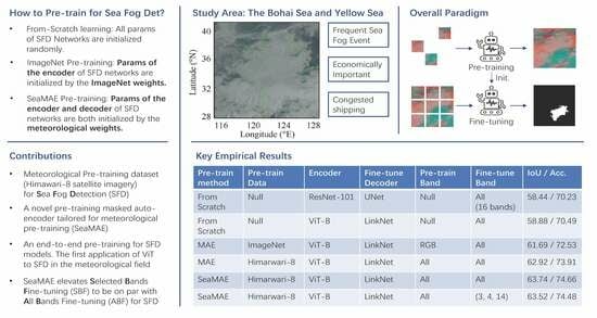
1. Introduction
- This paper proposes meteorological pre-training for sea fog detection (SFD). To this end, we collect 514,655 Himawari-8 satellite multi-channel images and use MAE to learn representations from them. On SFD, this pre-training paradigm outperforms from-scratch learning, ImageNet pre-training, and VHR satellite imagery pre-training. The power of available large-scale meteorological satellite raw data is unparalleledly utilized.
- We investigate a decoder architecture tailored for meteorological pre-training, which results in a novel variant of MAE, SeaMAE. Specifically, an off-shelf decoder effective in SFD is utilized to model masked patches in pre-training. Meteorological pre-training on the proposed SeaMAE facilitates additional performance gains for SFD. To our knowledge, this paper first pioneers the application of Vision Transformers for SFD in this community.
- SeaMAE intrinsically introduces an architecturally end-to-end pre-training paradigm, wherein the decoders in both pre-training and fine-tuning share the same architecture, revolutionizing the previous routine that only the encoder of SFD is pre-trained. We manifest that the pre-trained decoder performs better than the from-scratch learning decoder on fine-tuning data. The extension of pre-trained components in the SFD network shows great promise.
- Finally, training SFD networks typically involves using either all bands or (3, 4, 14) bands. Generally, the former performs better than the latter. Our proposed learning paradigm can adapt to both training settings, and make the latter performance on par with the former because our proposed learning paradigm has learned representations from all bands during the pre-training.
2. Materials and Methods
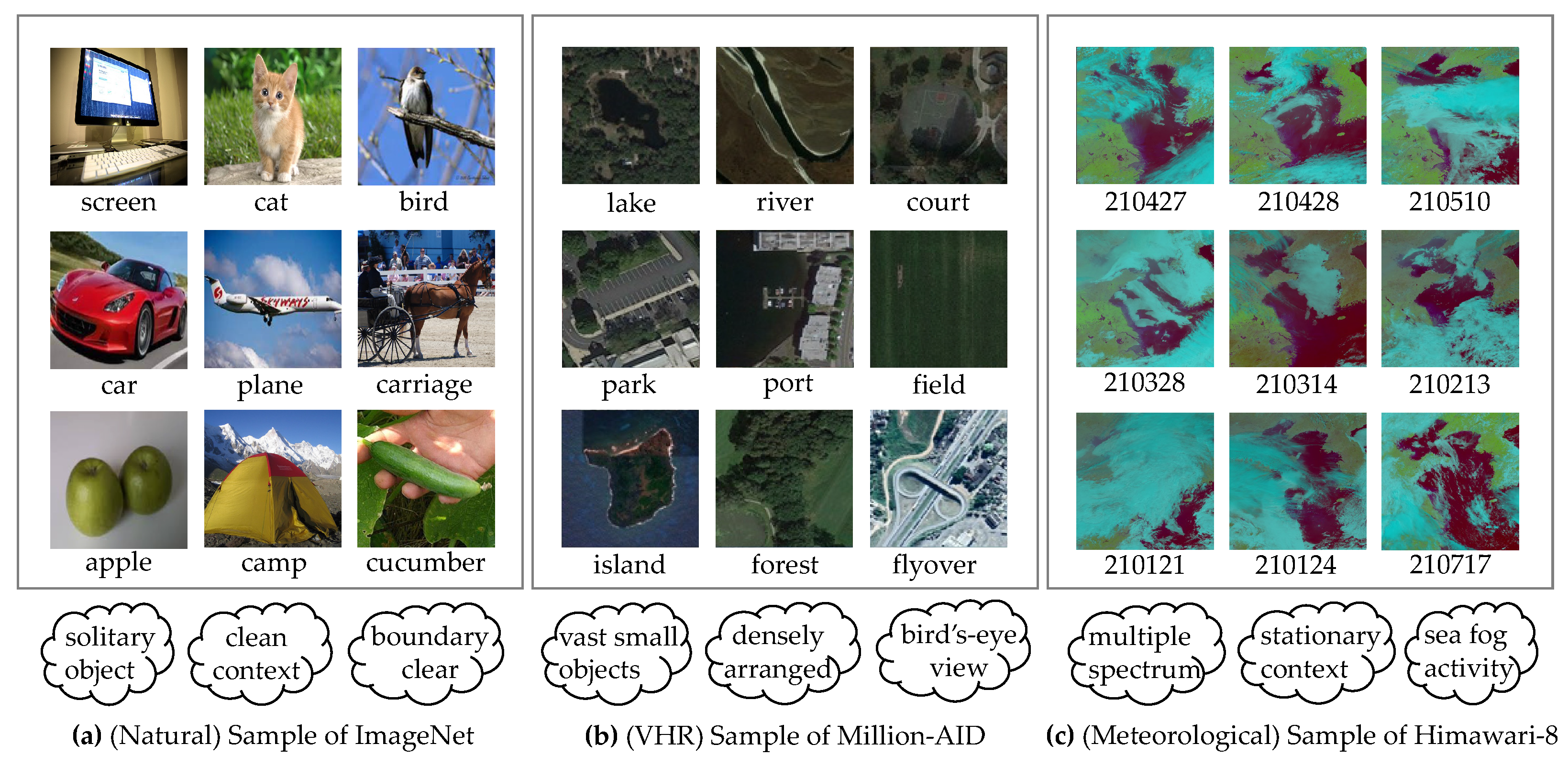
2.1. Himawari-8 Meteorological Satellite Imagery
2.1.1. Pre-Training Dataset
2.1.2. Fine-Tuning Dataset
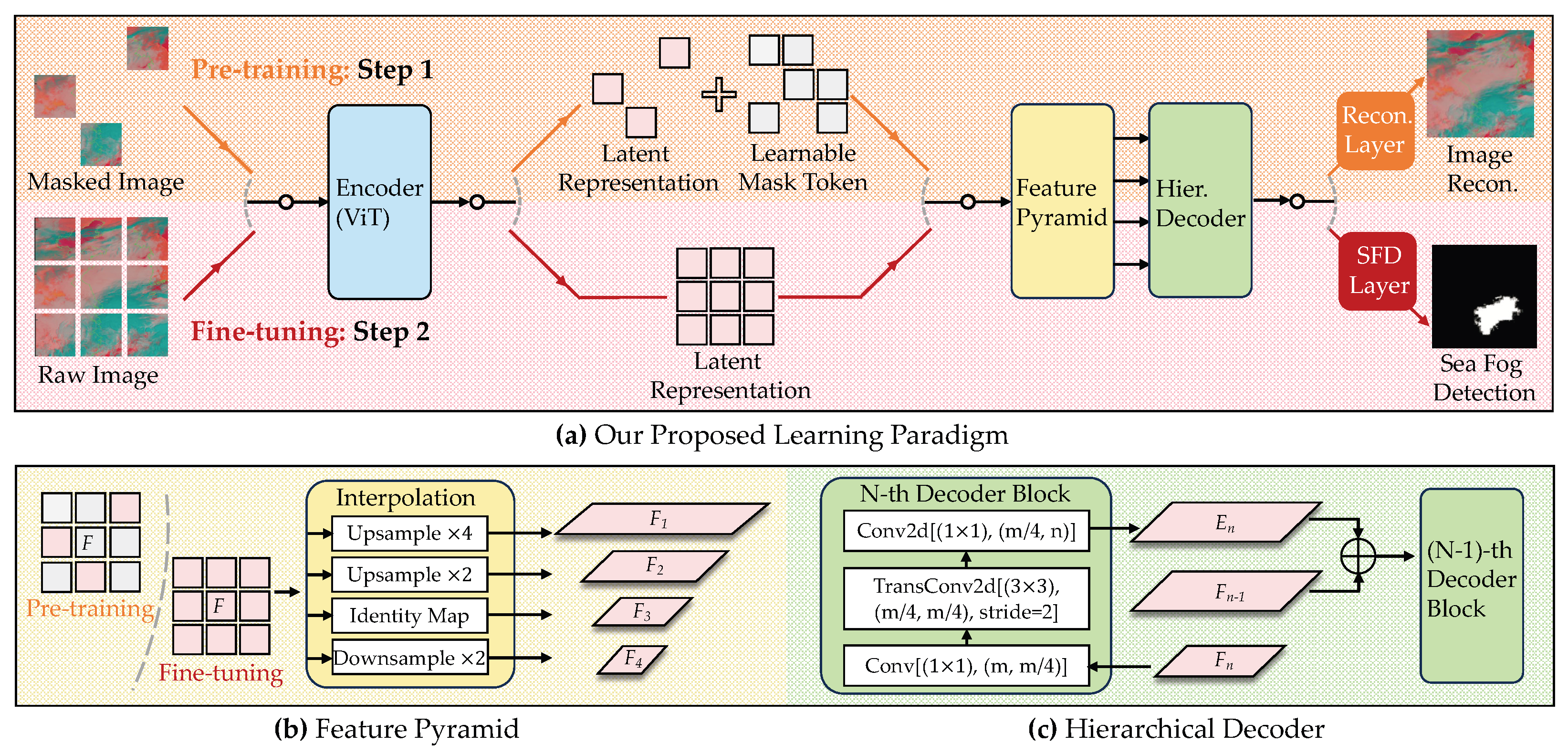
2.2. SeaMAE
2.2.1. SFD Driven by ViT
2.2.2. Hierarchical Decoder
2.2.3. Skip Connection for Masked Input
2.3. Learning Paradigm
3. Results
3.1. Implementation and Metric
3.2. MAE Pre-Training on Meteorological Satellite Imagery
3.3. SeaMAE Pre-Training on Meteorological Satellite Imagery
3.4. Ablation Study
3.4.1. End-to-End Pre-Training
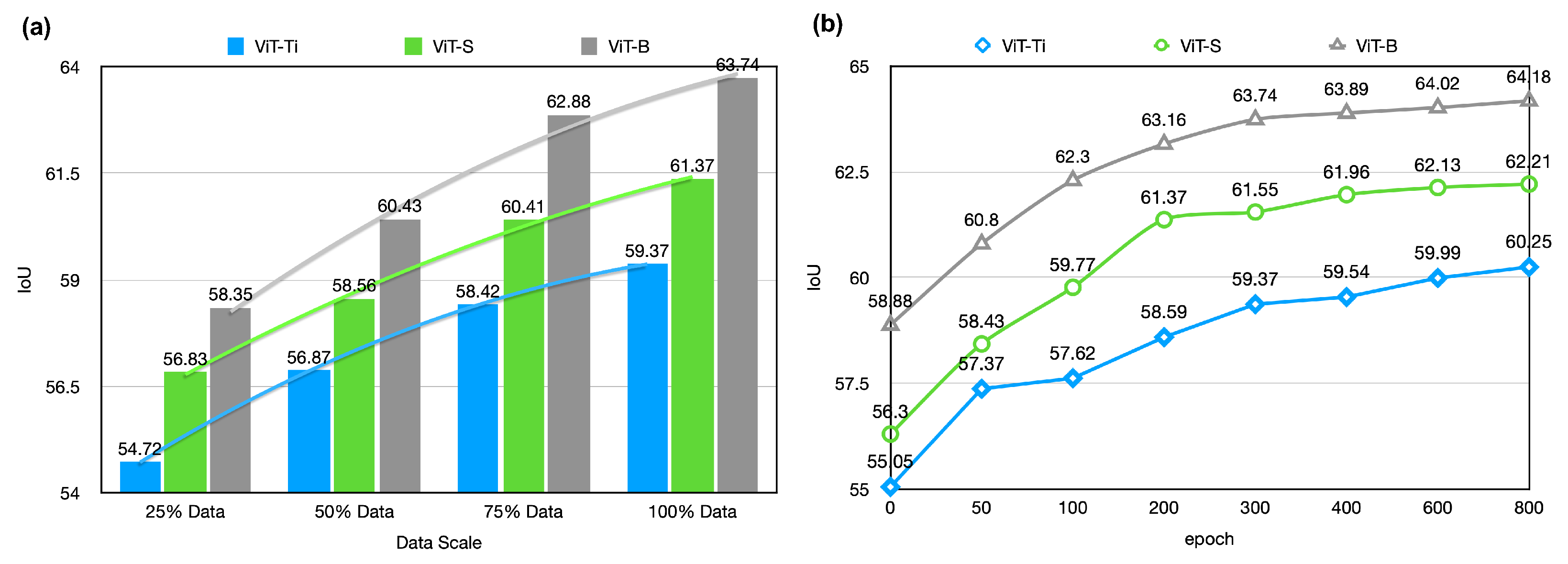
3.4.2. Data Scalability and Pre-Training Time
3.4.3. Band Number of Input
3.5. Comparison to Other Satellite Imagery Pre-Training Methods
3.6. Qualitative Results of Sea Fog Detection
3.7. Visualization
Qualitative Results of MIM
4. Discussions
4.1. Explanation of Results
4.2. Validation over 2021 Sea Fog Events
4.3. Literature Review and Comparison to Ours
4.3.1. Sea Fog Detection in Bohai Sea and Yellow Sea
4.3.2. MIM Pre-Training with Satellite Imagery
4.4. Future Directions
5. Conclusions
Author Contributions
Funding
Data Availability Statement
Conflicts of Interest
References
- Liu, X.; Ruan, Z.; Hu, S.; Wan, Q.; Liu, L.; Luo, Y.; Hu, Z.; Li, H.; Xiao, H.; Lei, W.; et al. The Longmen cloud physics field experiment base, China Meteorological Administration. J. Trop. Meteorol. 2023, 29, 1–15. [Google Scholar]
- Finnis, J.; Reid-Musson, E. Managing weather & fishing safety: Marine meteorology and fishing decision-making from a governance and safety perspective. Mar. Policy 2022, 142, 105120. [Google Scholar]
- Guo, X.; Wan, J.; Liu, S.; Xu, M.; Sheng, H.; Yasir, M. A scse-linknet deep learning model for daytime sea fog detection. Remote Sens. 2021, 13, 5163. [Google Scholar] [CrossRef]
- Zhu, C.; Wang, J.; Liu, S.; Sheng, H.; Xiao, Y. Sea fog detection using U-Net deep learning model based on MODIS data. In Proceedings of the 2019 10th Workshop on Hyperspectral Imaging and Signal Processing: Evolution in Remote Sensing (WHISPERS), Amsterdam, The Netherlands, 24–26 September 2019; pp. 1–5. [Google Scholar]
- Hu, T.; Jin, Z.; Yao, W.; Lv, J.; Jin, W. Cloud Image Retrieval for Sea Fog Recognition (CIR-SFR) Using Double Branch Residual Neural Network. IEEE J. Sel. Top. Appl. Earth Obs. Remote Sens. 2023, 16, 3174–3186. [Google Scholar] [CrossRef]
- Huang, Y.; Wu, M.; Guo, J.; Zhang, C.; Xu, M. A correlation context-driven method for sea fog detection in meteorological satellite imagery. IEEE Geosci. Remote Sens. Lett. 2021, 19, 1–5. [Google Scholar] [CrossRef]
- Jeon, H.K.; Kim, S.; Edwin, J.; Yang, C.S. Sea fog identification from GOCI images using CNN transfer learning models. Electronics 2020, 9, 311. [Google Scholar] [CrossRef]
- Li, T.; Jin, W.; Fu, R.; He, C. Daytime sea fog monitoring using multimodal self-supervised learning with band attention mechanism. Neural Comput. Appl. 2022, 34, 21205–21222. [Google Scholar] [CrossRef]
- Mahdavi, S.; Amani, M.; Bullock, T.; Beale, S. A probability-based daytime algorithm for sea fog detection using GOES-16 imagery. IEEE J. Sel. Top. Appl. Earth Obs. Remote Sens. 2020, 14, 1363–1373. [Google Scholar] [CrossRef]
- Xu, M.; Wu, M.; Guo, J.; Zhang, C.; Wang, Y.; Ma, Z. Sea fog detection based on unsupervised domain adaptation. Chin. J. Aeronaut. 2022, 35, 415–425. [Google Scholar] [CrossRef]
- Ryu, H.S.; Hong, S. Sea fog detection based on Normalized Difference Snow Index using advanced Himawari imager observations. Remote Sens. 2020, 12, 1521. [Google Scholar] [CrossRef]
- Tang, Y.; Yang, P.; Zhou, Z.; Zhao, X. Daytime Sea Fog Detection Based on a Two-Stage Neural Network. Remote Sens. 2022, 14, 5570. [Google Scholar] [CrossRef]
- Wan, J.; Su, J.; Sheng, H.; Liu, S.; Li, J. Spatial and temporal characteristics of sea fog in Yellow Sea and Bohai Sea based on active and passive remote sensing. In Proceedings of the IGARSS 2020—2020 IEEE International Geoscience and Remote Sensing Symposium, Waikoloa, HI, USA, 26 September–2 October 2020; pp. 5477–5480. [Google Scholar]
- Zhu, X.; Xu, M.; Wu, M.; Zhang, C.; Zhang, B. Annotating Only at Definite Pixels: A Novel Weakly Supervised Semantic Segmentation Method for Sea Fog Recognition. In Proceedings of the 2022 IEEE International Conference on Visual Communications and Image Processing (VCIP), Suzhou, China, 13–16 December 2022; pp. 1–5. [Google Scholar]
- He, K.; Chen, X.; Xie, S.; Li, Y.; Dollár, P.; Girshick, R. Masked autoencoders are scalable vision learners. In Proceedings of the IEEE/CVF Conference on Computer Vision and Pattern Recognition, New Orleans, LA, USA, 18–24 June 2022; pp. 16000–16009. [Google Scholar]
- Bao, H.; Dong, L.; Piao, S.; Wei, F. Beit: Bert pre-training of image transformers. arXiv 2021, arXiv:2106.08254. [Google Scholar]
- He, K.; Fan, H.; Wu, Y.; Xie, S.; Girshick, R. Momentum contrast for unsupervised visual representation learning. In Proceedings of the IEEE/CVF Conference on Computer Vision and Pattern Recognition, Seattle, WA, USA, 13–19 June 2020; pp. 9729–9738. [Google Scholar]
- Radford, A.; Kim, J.W.; Hallacy, C.; Ramesh, A.; Goh, G.; Agarwal, S.; Sastry, G.; Askell, A.; Mishkin, P.; Clark, J.; et al. Learning transferable visual models from natural language supervision. In Proceedings of the International Conference on Machine Learning, PMLR, Virtual, 18–24 July 2021; pp. 8748–8763. [Google Scholar]
- Chen, Z.; Agarwal, D.; Aggarwal, K.; Safta, W.; Balan, M.M.; Brown, K. Masked image modeling advances 3d medical image analysis. In Proceedings of the IEEE/CVF Winter Conference on Applications of Computer Vision, Waikoloa, HI, USA, 2–7 January 2023; pp. 1970–1980. [Google Scholar]
- Zhou, L.; Liu, H.; Bae, J.; He, J.; Samaras, D.; Prasanna, P. Self pre-training with masked autoencoders for medical image analysis. arXiv 2022, arXiv:2203.05573. [Google Scholar]
- Cong, Y.; Khanna, S.; Meng, C.; Liu, P.; Rozi, E.; He, Y.; Burke, M.; Lobell, D.; Ermon, S. Satmae: Pre-training transformers for temporal and multi-spectral satellite imagery. Adv. Neural Inf. Process. Syst. 2022, 35, 197–211. [Google Scholar]
- Sun, X.; Wang, P.; Lu, W.; Zhu, Z.; Lu, X.; He, Q.; Li, J.; Rong, X.; Yang, Z.; Chang, H.; et al. Ringmo: A remote sensing foundation model with masked image modeling. IEEE Trans. Geosci. Remote Sens. 2022, 61, 5612822. [Google Scholar] [CrossRef]
- Bessho, K.; Date, K.; Hayashi, M.; Ikeda, A.; Imai, T.; Inoue, H.; Kumagai, Y.; Miyakawa, T.; Murata, H.; Ohno, T.; et al. An introduction to Himawari-8/9—Japan’s new-generation geostationary meteorological satellites. J. Meteorol. Soc. Jpn. Ser. II 2016, 94, 151–183. [Google Scholar] [CrossRef]
- Deng, J.; Dong, W.; Socher, R.; Li, L.J.; Li, K.; Fei-Fei, L. Imagenet: A large-scale hierarchical image database. In Proceedings of the 2009 IEEE Conference on Computer Vision and Pattern Recognition, Miami, FL, USA, 20–25 June 2009; pp. 248–255. [Google Scholar]
- Dosovitskiy, A.; Beyer, L.; Kolesnikov, A.; Weissenborn, D.; Zhai, X.; Unterthiner, T.; Dehghani, M.; Minderer, M.; Heigold, G.; Gelly, S.; et al. An image is worth 16 × 16 words: Transformers for image recognition at scale. arXiv 2020, arXiv:2010.11929. [Google Scholar]
- Chaurasia, A.; Culurciello, E. Linknet: Exploiting encoder representations for efficient semantic segmentation. In Proceedings of the 2017 IEEE Visual Communications and Image Processing (VCIP), St. Petersburg, FL, USA, 10–13 December 2017; pp. 1–4. [Google Scholar]
- Zhou, L.; Zhang, C.; Wu, M. D-LinkNet: LinkNet with pretrained encoder and dilated convolution for high resolution satellite imagery road extraction. In Proceedings of the IEEE Conference on Computer Vision and Pattern Recognition Workshops, Salt Lake City, UT, USA, 18–23 June 2018; pp. 182–186. [Google Scholar]
- Chen, L.C.; Zhu, Y.; Papandreou, G.; Schroff, F.; Adam, H. Encoder-decoder with atrous separable convolution for semantic image segmentation. In Proceedings of the European Conference on Computer Vision (ECCV), Munich, Germany, 8–14 September 2018; pp. 801–818. [Google Scholar]
- Zhou, Z.; Rahman Siddiquee, M.M.; Tajbakhsh, N.; Liang, J. Unet++: A nested u-net architecture for medical image segmentation. In Deep Learning in Medical Image Analysis and Multimodal Learning for Clinical Decision Support 4th International Workshop, Proceedings of the DLMIA 2018, and 8th International Workshop, ML-CDS 2018, Held in Conjunction with MICCAI 2018, Granada, Spain, 20 September 2018; Springer: Cham, Switzerland, 2018; pp. 3–11. [Google Scholar]
- Oktay, O.; Schlemper, J.; Folgoc, L.L.; Lee, M.; Heinrich, M.; Misawa, K.; Mori, K.; McDonagh, S.; Hammerla, N.Y.; Kainz, B.; et al. Attention u-net: Learning where to look for the pancreas. arXiv 2018, arXiv:1804.03999. [Google Scholar]
- Ronneberger, O.; Fischer, P.; Brox, T. U-net: Convolutional networks for biomedical image segmentation. In Proceedings of the Medical Image Computing and Computer-Assisted Intervention–MICCAI 2015: 18th International Conference, Munich, Germany, 5–9 October 2015; Springer: Cham, Switzerland, 2015. Proceedings, Part III 18. pp. 234–241. [Google Scholar]
- He, K.; Zhang, X.; Ren, S.; Sun, J. Deep residual learning for image recognition. In Proceedings of the IEEE Conference on Computer Vision and Pattern Recognition, Las Vegas, NV, USA, 27–30 June 2016; pp. 770–778. [Google Scholar]
- Li, Y.; Xie, S.; Chen, X.; Dollar, P.; He, K.; Girshick, R. Benchmarking detection transfer learning with vision transformers. arXiv 2021, arXiv:2111.11429. [Google Scholar]
- Feichtenhofer, C.; Li, Y.; He, K. Masked autoencoders as spatiotemporal learners. Adv. Neural Inf. Process. Syst. 2022, 35, 35946–35958. [Google Scholar]
- Zhou, J.; Wei, C.; Wang, H.; Shen, W.; Xie, C.; Yuille, A.; Kong, T. ibot: Image bert pre-training with online tokenizer. arXiv 2021, arXiv:2111.07832. [Google Scholar]
- Yu, X.; Tang, L.; Rao, Y.; Huang, T.; Zhou, J.; Lu, J. Point-bert: Pre-training 3d point cloud transformers with masked point modeling. In Proceedings of the IEEE/CVF Conference on Computer Vision and Pattern Recognition, New Orleans, LA, USA, 18–24 June 2022; pp. 19313–19322. [Google Scholar]
- Wang, R.; Chen, D.; Wu, Z.; Chen, Y.; Dai, X.; Liu, M.; Jiang, Y.G.; Zhou, L.; Yuan, L. Bevt: Bert pretraining of video transformers. In Proceedings of the IEEE/CVF Conference on Computer Vision and Pattern Recognition, New Orleans, LA, USA, 18–24 June 2022; pp. 14733–14743. [Google Scholar]
- He, Q.; Sun, X.; Yan, Z.; Wang, B.; Zhu, Z.; Diao, W.; Yang, M.Y. AST: Adaptive Self-supervised Transformer for optical remote sensing representation. ISPRS J. Photogramm. Remote Sens. 2023, 200, 41–54. [Google Scholar] [CrossRef]
- Wang, D.; Zhang, Q.; Xu, Y.; Zhang, J.; Du, B.; Tao, D.; Zhang, L. Advancing plain vision transformer towards remote sensing foundation model. IEEE Trans. Geosci. Remote Sens. 2022, 61, 5607315. [Google Scholar] [CrossRef]
- Tseng, G.; Zvonkov, I.; Purohit, M.; Rolnick, D.; Kerner, H. Lightweight, Pre-trained Transformers for Remote Sensing Timeseries. arXiv 2023, arXiv:2304.14065. [Google Scholar]
- Scheibenreif, L.; Mommert, M.; Borth, D. Masked Vision Transformers for Hyperspectral Image Classification. In Proceedings of the IEEE/CVF Conference on Computer Vision and Pattern Recognition, Vancouver, BC, Canada, 24–31 January 2023; pp. 2165–2175. [Google Scholar]
- Jain, P.; Schoen-Phelan, B.; Ross, R. Self-supervised learning for invariant representations from multi-spectral and sar images. IEEE J. Sel. Top. Appl. Earth Obs. Remote Sens. 2022, 15, 7797–7808. [Google Scholar] [CrossRef]
- Marsocci, V.; Scardapane, S. Continual Barlow Twins: Continual self-supervised learning for remote sensing semantic segmentation. IEEE J. Sel. Top. Appl. Earth Obs. Remote Sens. 2023, 16, 5049–5060. [Google Scholar] [CrossRef]
- Mikriukov, G.; Ravanbakhsh, M.; Demir, B. Deep unsupervised contrastive hashing for large-scale cross-modal text-image retrieval in remote sensing. arXiv 2022, arXiv:2201.08125. [Google Scholar]
- Wanyan, X.; Seneviratne, S.; Shen, S.; Kirley, M. DINO-MC: Self-supervised Contrastive Learning for Remote Sensing Imagery with Multi-sized Local Crops. arXiv 2023, arXiv:2303.06670. [Google Scholar]
- Li, W.; Chen, K.; Chen, H.; Shi, Z. Geographical knowledge-driven representation learning for remote sensing images. IEEE Trans. Geosci. Remote Sens. 2021, 60, 5405516. [Google Scholar] [CrossRef]
- Muhtar, D.; Zhang, X.; Xiao, P. Index your position: A novel self-supervised learning method for remote sensing images semantic segmentation. IEEE Trans. Geosci. Remote Sens. 2022, 60, 4411511. [Google Scholar] [CrossRef]
- Mall, U.; Hariharan, B.; Bala, K. Change-Aware Sampling and Contrastive Learning for Satellite Images. In Proceedings of the IEEE/CVF Conference on Computer Vision and Pattern Recognition, Vancouver, BC, Canada, 24–31 January 2023; pp. 5261–5270. [Google Scholar]
- Manas, O.; Lacoste, A.; Giró-i Nieto, X.; Vazquez, D.; Rodriguez, P. Seasonal contrast: Unsupervised pre-training from uncurated remote sensing data. In Proceedings of the IEEE/CVF International Conference on Computer Vision, Montreal, BC, Canada, 11–17 October 2021; pp. 9414–9423. [Google Scholar]
- Jain, P.; Schoen-Phelan, B.; Ross, R. Multi-modal self-supervised representation learning for earth observation. In Proceedings of the 2021 IEEE International Geoscience and Remote Sensing Symposium IGARSS, Brussels, Belgium, 11–16 July 2021; pp. 3241–3244. [Google Scholar]
- Jain, U.; Wilson, A.; Gulshan, V. Multimodal contrastive learning for remote sensing tasks. arXiv 2022, arXiv:2209.02329. [Google Scholar]
- Prexl, J.; Schmitt, M. Multi-Modal Multi-Objective Contrastive Learning for Sentinel-1/2 Imagery. In Proceedings of the IEEE/CVF Conference on Computer Vision and Pattern Recognition, Montreal, BC, Canada, 11–17 October 2023; pp. 2135–2143. [Google Scholar]
- Akiva, P.; Purri, M.; Leotta, M. Self-supervised material and texture representation learning for remote sensing tasks. In Proceedings of the IEEE/CVF Conference on Computer Vision and Pattern Recognition, New Orleans, LA, USA, 18–24 June 2022; pp. 8203–8215. [Google Scholar]
- Li, W.; Chen, H.; Shi, Z. Semantic segmentation of remote sensing images with self-supervised multitask representation learning. IEEE J. Sel. Top. Appl. Earth Obs. Remote Sens. 2021, 14, 6438–6450. [Google Scholar] [CrossRef]
- Tao, C.; Qi, J.; Zhang, G.; Zhu, Q.; Lu, W.; Li, H. TOV: The original vision model for optical remote sensing image understanding via self-supervised learning. IEEE J. Sel. Top. Appl. Earth Obs. Remote Sens. 2023, 16, 4916–4930. [Google Scholar] [CrossRef]
- Scheibenreif, L.; Hanna, J.; Mommert, M.; Borth, D. Self-supervised vision transformers for land-cover segmentation and classification. In Proceedings of the IEEE/CVF Conference on Computer Vision and Pattern Recognition, New Orleans, LA, USA, 18–24 June 2022; pp. 1422–1431. [Google Scholar]


| No. | Name | Type | Detection Category |
|---|---|---|---|
| B01 | V1 | Visible | Vegetation, aerosol |
| B02 | V2 | Visible | Vegetation, aerosol |
| B03 | VS | Visible | Low cloud (fog) |
| B04 | N1 | Near Infrared | Vegetation, aerosol |
| B05 | N2 | Near Infrared | Cloud phase recognition |
| B06 | N3 | Near Infrared | Cloud droplet effective radius |
| B07 | I4 | Infrared | Low cloud (fog), natural disaster |
| B08 | WV | Infrared | Water vapor density from troposphere to mesosphere |
| B09 | W2 | Infrared | Water vapor density in the mesosphere |
| B10 | W3 | Infrared | Water vapor density in the mesosphere |
| B11 | MI | Infrared | Cloud phase discrimination, sulfur dioxide |
| B12 | O3 | Infrared | Ozone content |
| B13 | IR | Infrared | Cloud image, cloud top |
| B14 | L2 | Infrared | Cloud image, sea surface temperature |
| B15 | I2 | Infrared | Cloud image, sea surface temperature |
| B16 | CO | Infrared | Cloud height |
| Backbone | Methods | IoU | Acc |
|---|---|---|---|
| Deeplabv3+ [28] | 56.10 | 68.89 | |
| Scselinknet [3] | 55.29 | 68.18 | |
| CNN | UNet [31] | 58.44 | 70.23 |
| UNet++ [29] | 56.95 | 69.30 | |
| Attetion-unet [30] | 56.35 | 68.94 |
| Pre-Train Method | Pre-Train Data | Encoder | Fine-Tune Decoder | IoU | Acc. |
|---|---|---|---|---|---|
| Supervised | ImageNet | CNN | UNet | 58.44 | 70.23 |
| From Scratch | — | ViT-Ti | LinkNet | 55.05 | 66.48 |
| MAE | ImageNet | ViT-Ti | LinkNet | 57.79 | 69.78 |
| MAE | Million-AID | ViT-Ti | LinkNet | 57.56 | 69.63 |
| MAE | Himawari-8 | ViT-Ti | LinkNet | 58.63 (+1.07) | 70.47 (+0.84) |
| From Scratch | — | ViT-S | LinkNet | 56.30 | 68.04 |
| MAE | ImageNet | ViT-S | LinkNet | 59.42 | 70.82 |
| MAE | Million-AID | ViT-S | LinkNet | 59.62 | 71.35 |
| MAE | Himawari-8 | ViT-S | LinkNet | 60.48 (+0.86) | 71.87 (+0.52) |
| From Scratch | — | ViT-B | LinkNet | 58.88 | 70.49 |
| MAE | ImageNet | ViT-B | LinkNet | 61.69 | 72.53 |
| MAE | Million-AID | ViT-B | LinkNet | 61.87 | 72.79 |
| MAE | Himawari-8 | ViT-B | LinkNet | 62.92 (+1.05) | 73.91 (+1.12) |
| Pre-Train Method | Pre-Train Data | Encoder | Skip Connection | IoU | Acc. |
|---|---|---|---|---|---|
| MAE | Himawari-8 | ViT-Ti | – | 58.63 | 70.47 |
| SeaMAE | Himawari-8 | ViT-Ti | ✓ | 59.37 (+0.74) | 70.97 (+0.50) |
| SeaMAE | Himawari-8 | ViT-Ti | ✗ | 59.09 (−0.28) | 70.71 (−0.28) |
| MAE | Himawari-8 | ViT-S | – | 60.48 | 71.87 |
| SeaMAE | Himawari-8 | ViT-S | ✓ | 61.55 (+1.07) | 72.52 (+0.95) |
| SeaMAE | Himawari-8 | ViT-S | ✗ | 61.12 (−0.43) | 72.24 (−0.28) |
| MAE | Himawari-8 | ViT-B | – | 62.92 | 73.91 |
| SeaMAE | Himawari-8 | ViT-B | ✓ | 63.74 (+0.82) | 75.12 (+1.21) |
| SeaMAE | Himawari-8 | ViT-B | ✗ | 63.37 (−0.37) | 74.66 (−0.48) |
| Encoder Init. | Decoder Init. | Encoder | IoU | Acc. |
|---|---|---|---|---|
| MAE | Random | ViT-Ti | 58.63 | 70.47 |
| SeaMAE | Random | ViT-Ti | 59.16 | 70.94 |
| SeaMAE | SeaMAE | ViT-Ti | 59.37 (+0.21) | 70.97 (+0.03) |
| MAE | Random | ViT-S | 60.48 | 71.87 |
| SeaMAE | Random | ViT-S | 61.02 | 72.16 |
| SeaMAE | SeaMAE | ViT-S | 61.55 (+0.53) | 72.52 (+0.36) |
| MAE | Random | ViT-B | 62.92 | 73.91 |
| SeaMAE | Random | ViT-B | 63.43 | 74.25 |
| SeaMAE | SeaMAE | ViT-B | 63.74 (+0.31) | 74.66 (+0.41) |
| Pre-Train Band# | Fine-Tune Band# | Patch Emb. Adjustment | IoU | Acc. |
|---|---|---|---|---|
| 16 | 16 | — | 63.74 | 74.66 |
| 3 | 3 | — | 63.08 (−0.66 ) | 73.99 (−0.67) |
| 16 | 3 | Random | 62.59 (−1.15) | 73.43 (−1.23) |
| 16 | 3 | Index | 62.71 (−1.03) | 73.50 (−1.16) |
| 16 | 3 | Resize | 63.52 (−0.22) | 74.48 (−0.18) |
| Pre-Train Method | Pre-Train Data | Encoder | IoU | Acc. |
|---|---|---|---|---|
| SatMAE | Himawari-8 | ViT-Ti | 58.56 | 70.28 |
| RingMo | Himawari-8 | ViT-Ti | 58.22 | 69.90 |
| SeaMAE | Himawari-8 | ViT-Ti | 59.37 (+0.81) | 70.97 (+0.69) |
| SatMAE | Himawari-8 | ViT-S | 60.26 | 71.55 |
| RingMo | Himawari-8 | ViT-S | 60.14 | 71.61 |
| SeaMAE | Himawari-8 | ViT-S | 61.55 (+1.29) | 72.52 (+0.91) |
| SatMAE | Himawari-8 | ViT-B | 62.83 | 74.39 |
| RingMo | Himawari-8 | ViT-B | 63.02 | 74.42 |
| SeaMAE | Himawari-8 | ViT-B | 63.74 (+0.72) | 75.12 (+0.70) |
| Jan. 21st | Jan. 24th | Jan. 26th | Feb. 11th | Feb. 12th | Feb. 13th |
|---|---|---|---|---|---|
| 8 h | 8 h | 8 h | 8 h | 8 h | 8 h |
| 49.69 | 40.52 | 61.70 | 76.51 | 61.32 | 46.43 |
| 74.28 (+24.59) | 64.86 (+24.34) | 72.75 (+11.05) | 77.63 (+1.12) | 63.93 (+2.61) | 59.59 (+13.16) |
| Feb. 20th | Mar. 5th | Mar. 10th | Mar. 14th | Mar. 25th | Mar. 28th |
| 8 h | 8 h | 8 h | 8 h | 8 h | 8 h |
| 54.05 | 58.34 | 58.77 | 56.37 | 90.55 | 56.10 |
| 63.08 (+9.03) | 76.61 (+18.27) | 60.42 (+1.64) | 58.86 (+2.49) | 91.12 (+0.57) | 68.03 (+11.93) |
| Apr. 26th | Apr. 27th | Apr. 28th | Apr. 29th | May 9th | May 10th |
| 7.5 h | 8 h | 6.5 h | 6.5 h | 8 h | 8 h |
| 64.67 | 55.81 | 59.36 | 58.07 | 87.94 | 72.94 |
| 65.28 (+0.61) | 59.64 (+3.83) | 64.11 (+4.75) | 62.43 (+4.36) | 88.08 (+0.14) | 73.86 (+0.92) |
| May 30th | May 31st | Jun. 6th | Jun. 13th | Jul. 11th | Jul. 17th |
| 8 h | 8 h | 8 h | 8 h | 3 h | 5.5 h |
| 68.73 | 75.95 | 79.03 | 80.00 | 49.61 | 45.99 |
| 70.41 (+1.68) | 77.81 (+1.86) | 80.13 (+1.10) | 80.34 (+0.34) | 64.96 (+15.35) | 68.44 (+22.45) |
| Winter | Spring | Summer | ||||
|---|---|---|---|---|---|---|
| Jan. | Feb. | Mar. | Apr. | May | Jun. | Jul. |
| 3 | 3 | 5 | 4 | 4 | 2 | 2 |
Disclaimer/Publisher’s Note: The statements, opinions and data contained in all publications are solely those of the individual author(s) and contributor(s) and not of MDPI and/or the editor(s). MDPI and/or the editor(s) disclaim responsibility for any injury to people or property resulting from any ideas, methods, instructions or products referred to in the content. |
© 2023 by the authors. Licensee MDPI, Basel, Switzerland. This article is an open access article distributed under the terms and conditions of the Creative Commons Attribution (CC BY) license (https://creativecommons.org/licenses/by/4.0/).
Share and Cite
Yan, H.; Su, S.; Wu, M.; Xu, M.; Zuo, Y.; Zhang, C.; Huang, B. SeaMAE: Masked Pre-Training with Meteorological Satellite Imagery for Sea Fog Detection. Remote Sens. 2023, 15, 4102. https://doi.org/10.3390/rs15164102
Yan H, Su S, Wu M, Xu M, Zuo Y, Zhang C, Huang B. SeaMAE: Masked Pre-Training with Meteorological Satellite Imagery for Sea Fog Detection. Remote Sensing. 2023; 15(16):4102. https://doi.org/10.3390/rs15164102
Chicago/Turabian StyleYan, Haotian, Sundingkai Su, Ming Wu, Mengqiu Xu, Yihao Zuo, Chuang Zhang, and Bin Huang. 2023. "SeaMAE: Masked Pre-Training with Meteorological Satellite Imagery for Sea Fog Detection" Remote Sensing 15, no. 16: 4102. https://doi.org/10.3390/rs15164102
APA StyleYan, H., Su, S., Wu, M., Xu, M., Zuo, Y., Zhang, C., & Huang, B. (2023). SeaMAE: Masked Pre-Training with Meteorological Satellite Imagery for Sea Fog Detection. Remote Sensing, 15(16), 4102. https://doi.org/10.3390/rs15164102