Abstract
Digital terrain model (DTM) creation is a modeling process that represents the Earth’s surface. An aptly designed DTM generation method tailored for intended study can significantly streamline ensuing processes and assist in managing errors and uncertainties, particularly in large-area projects. However, existing methods often exhibit inconsistent and inexplicable results, struggle to clearly define what an object is, and often fail to filter large objects due to their locally confined operations. We introduce a new DTM generation method that performs object-based ground filtering, which is particularly beneficial for urban topography. This method defines objects as areas fully enclosed by steep slopes and grounds as smoothly connected areas, enabling reliable “object-based” segmentation and filtering, extending beyond the local context. Our primary operation, controlled by a slope threshold parameter, simplifies tuning and ensures predictable results, thereby reducing uncertainties in large-area modeling. Uniquely, our method considers surface water bodies in modeling and treats connected artificial terrains (e.g., overpasses) as ground. This contrasts with conventional methods, which often create noise near water bodies and behave inconsistently around overpasses and bridges, making our approach particularly beneficial for large-area 3D urban mapping. Examined on extensive and diverse datasets, our method offers unique features and high accuracy, and we have thoroughly assessed potential artifacts to guide potential users.
1. Introduction
A digital terrain model (DTM) represents a three-dimensional model of the ground surface excluding above-ground features such as buildings and trees. DTM is primarily used for serving as a basis terrain map for simulating and analyzing events occurring over large areas of the Earth, such as hydrological simulations [1], landslide monitoring [2,3], urban object mapping [4,5,6], glacier monitoring [7], and agricultural and forestry applications [8].
For creating a DTM, light detection and ranging (LiDAR) [9,10,11], radar [12], and photogrammetric methods [13,14,15] are generally used for collecting the three-dimensional coordinates of the earth. Then, the DTM generation method separates the bare earth from all other ground-standing objects on the earth’s surface. Among various data sources, airborne laser scanning (airborne LiDAR data) has been demonstrated to be the most effective method for creating precise DTMs across extensive areas.
Over the decades, numerous algorithms have been developed to generate DTMs from airborne LiDAR data [11,16]. However, algorithms and their implementations generally involve more than one of the following problems:
- Cannot consider beyond the local context: Algorithms filter the ground based on locally limited information. Specifically, filtering decisions are made based on either a local neighborhood (or a window in morphological filtering), a local ground surface (e.g., cloth simulation), or an image patch (i.e., input for deep learning-based methods). Thus, algorithms must make decisions considering only the data within a limited area, which poses a challenge in filtering large objects.
- Cannot clearly define what an object is: Algorithms typically analyze geometrical features to perform filtering on a smaller-than-object basis but cannot clearly define an object to filter an entire object at once. Alternatively, algorithms try to simulate the ground surface itself or infer the object through deep learning models without explicitly defining objects.
- Require frequent parameter tunings: For the algorithm to work properly, parameters must be tuned for each local landscape. Parameter settings are sometimes not intuitive and require a lot of trial and error.
- Results are unexplainable and unpredictable: Complex filtering rules and intricate interactions among numerous parameters often obscure the algorithm’s decision-making process, leading to significant uncertainties in large-area mapping.
- Ignoring water bodies: The topography includes both terrains and water bodies. Despite their interaction and influence on each other’s shape, previous literature often neglects water bodies and their effects on terrain mapping quality.
- Require high-quality training samples: Deep learning algorithms necessitate numerous training samples, and the resulting DTM quality heavily relies on the reference DTM used for training.
- Limited availability/High computation: Few methods are open-source, and most are computationally expensive, making them unsuitable for large-area mapping.
Notably, DTM generation is a modeling process; therefore, there is no definitive ground truth or absolute answer. However, researchers strive to find easy-to-use methods that are suitable for the objectives of follow-up studies and that produce reliable and consistent results [11,16,17]. Furthermore, as DTM is often created for large areas, quality control can be challenging, further emphasizing the need for a method with straightforward rules that yields easy-to-predict and consistent outcomes.
This paper presents an object-based ground filtering DTM generation method that operates based on connectivity, beyond local constraints. Our method provides a clear definition of objects as areas that are fully enclosed by steep slopes, while grounds are defined as areas where all grounds are eventually connected smoothly to each other. Our primary operation in ground filtering is controlled by a single parameter, “slope threshold ()” that defines the steep slope. The parameter tuning is intuitive, and the outcomes are easily interpretable. Our method offers several unique features, considering surface water bodies and treating connected artificial terrains (e.g., overpasses) as ground surfaces, unlike other methods that produce noises near water bodies and show inconsistent behaviors in overpasses. The proposed method underwent extensive evaluation in large areas and was compared to state-of-the-art methods. We confirmed that our method’s scalability is advantageous for large-area terrain modeling, with its unique feature being especially beneficial for 3D urban modeling.
2. Related Works
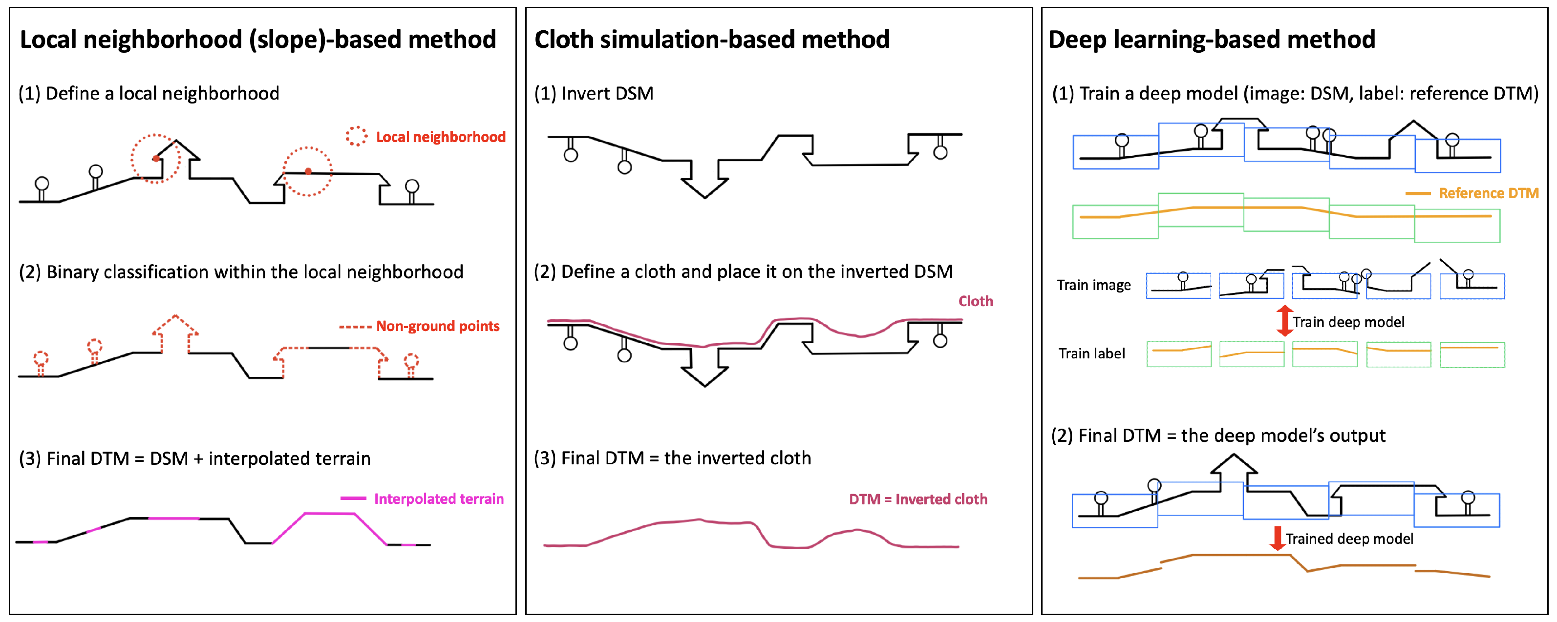
DTM generation methods can be categorized into three main types: (1) local neighborhood (slope)-based, (2) cloth simulation-based, and (3) deep learning-based methods. Figure 1 illustrates the basic principles of each category. Please refer to [11,16,18] for a comprehensive review.
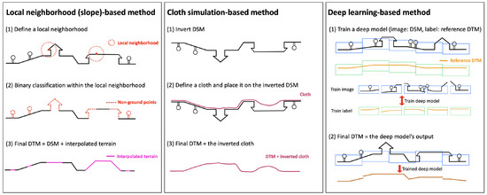
Figure 1.
A graphical illustration of representative DTM generation methods. All methods cannot explicitly define what an object is, and their filtering decisions are made based on locally limited information (i.e., local neighborhood, local surface, and an input patch for deep learning models).
Local neighborhood (slope)-based methods [19,20,21,22,23,24,25,26,27,28,29,30,31,32,33] set a local neighborhood for a point of interest and then classify whether each point is ground or non-ground based on the relative coordinates of the points belonging to the local neighborhood. The point and its local neighborhood could be other types of point cloud representations such as a triangulated irregular network (TIN) and a window or kernel in a digital surface model (DSM).
Local neighborhood (slope)-based methods assume the ground is planar and non-ground objects exhibit protruding geometry. Specifically, when the local neighborhood is defined with a set of points, the typical way is to find a planar surface, calculate geometrical features (e.g., slope or elevation difference), and consider outlying points from the planar surface as non-ground points [19]. With TIN representation, triangular facets approximate local surfaces, and non-ground points are filtered based on slope [20]. In DSM representation, kernel-based morphological operations filter non-ground pixels [21,26,28].
Whatever type of representation is adopted, the question is how large should the local neighborhood be and how to quantify planarity [11]. For instance, a flat-roofed building can only be filtered as non-ground if the local neighborhood extends beyond its boundaries; otherwise, central roof points may be misclassified as ground. Merely expanding the neighborhood radius is not always helpful as it increases the likelihood of including both smooth and protruding surfaces. This leads to a more complex algorithm, requiring extensive parameter tuning [18,34], which can ultimately degrade its generalization capability.
Cloth simulation-based methods [34,35,36,37,38] assume that the terrain can be modeled as a smooth surface placed on an inverted DSM. The method covers a simulated surface over the inverted DSM and considers the surface cover as an inverted terrain.
The cloth simulation-based filtering method proposed in the study [35] employs a grid of interconnected particles with mass to represent a cloth plane. This method has four main user-determined parameters: grid resolution (GR), rigidness (RI), time step (dT), and a steep slope fit factor (SSFT). GR establishes the spatial resolution, RI determines cloth rigidity, dT governs particle falling speed, and SSFT serves as a Boolean parameter for post-processing error mitigation.
While the cloth simulation-based method generally yields satisfactory results and requires less parameter tuning compared to the typical local neighborhood (slope)-based methods, it still necessitates iterative tuning for different landscapes [18,34,37]. Additionally, some parameters, such as rigidness, lack universal measurement units, making parameter tuning less intuitive.
Deep learning-based methods [39,40,41,42,43] treat DSM as an image and identify ground pixels using image recognition approaches, such as patch-based classifications [44] and semantic segmentations [45].
One study [39] employed a convolutional neural network (CNN) to classify the center pixel of an image patch as ground or non-ground, using DSM-based feature maps and 17 million labeled points. Another study [40] used RGB images and DSM-based feature maps as input to a deep model and trained it with automatically selected samples for DTM extraction. Another study [42] proposed a multi-scale DTM fusion strategy to minimize errors and obtain a seamless DTM surface, using the U.S. Geological Survey (USGS)-provided DTM for training labels.
Despite satisfactory results, deep learning-based methods require large labeled training samples and entail substantial computation costs. In addition, output quality is often constrained by both the LiDAR data as well as the reference training-DTM data. Moreover, trained models may not perform well in new environments due to the distribution shift.
3. Proposed DTM Generation Method
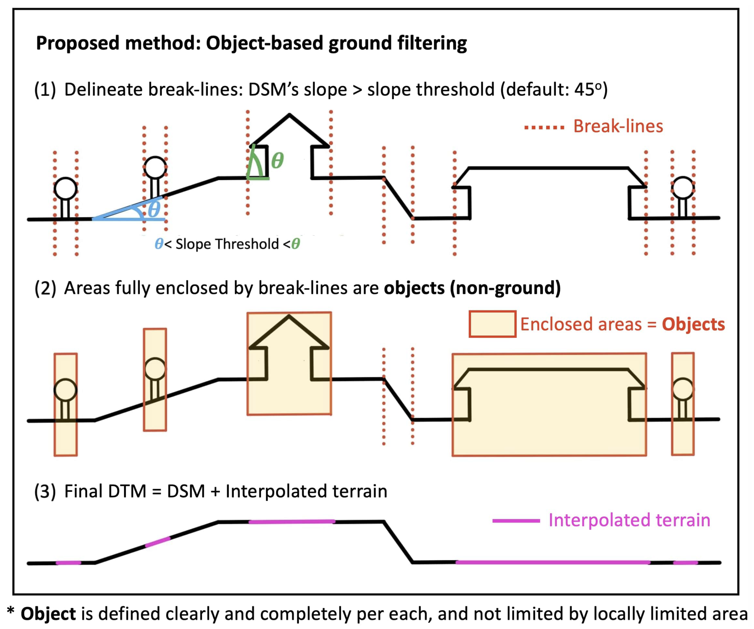
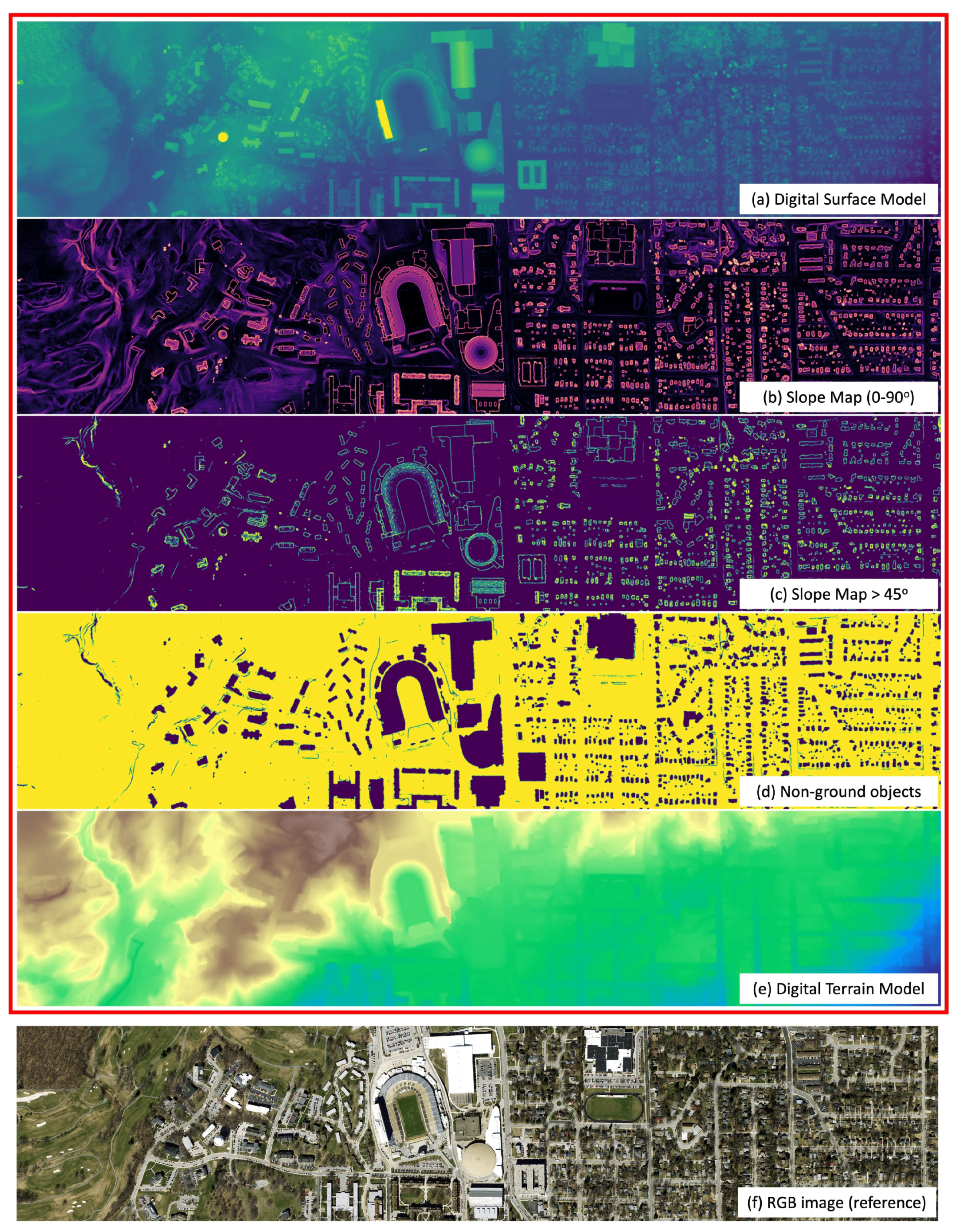
The proposed method consists of the following primary operations: (1) break-line delineation over the DSM, (2) (non-ground) object filtering using break-lines, and (3) creating the final DTM. For better comprehension, please refer to Figure 2 and Figure 3a–f.
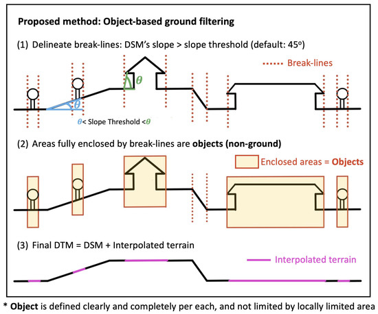
Figure 2.
A graphical illustration of our proposed method for DTM generation. An object is clearly defined as a “fully enclosed” area by break-lines, and the parameter (i.e., slope threshold) and the connectivity control the ground filtering rule. Since the enclosed area extends beyond the local context, large objects can be filtered robustly. (Figure 3 provides an aerial view of the procedure).
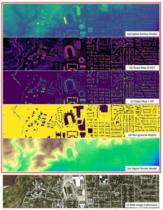
Figure 3.
A graphical procedure of the DTM generation using the proposed method. The proposed method filters objects by taking into account their connectivity based on break-lines, which are defined by the slope of the terrain. This approach enables object-wise filtering, providing clear definitions for objects and grounds. It performs effectively for objects of varying sizes, from small to large, thus facilitating scalable object mapping.
3.1. Break-Line Delineation
A key assumption of our method is that objects are surrounded by steep slopes. Thus, our process initiates by creating a slope map derived from the DSM. In this slope map, each pixel corresponds to the slope value in the rasterized DSM, computed using a Sobel operator [46,47]. Pixels demonstrating a slope exceeding a pre-defined slope threshold () are classified as break-lines, as shown in step 1 of Figure 2.
Given that the slope can be approximated from any type of DSM, the presence of a DSM is the only requirement for progressing to the following stages of our method. However, when a DSM is generated from point clouds, it is advisable to create a high-resolution DSM by capturing the last return (which corresponds to the lowest elevation point within the grid). Moreover, prior to the application of the Sobel operator, it is beneficial for this high-resolution DSM to undergo noise reduction with low-pass filtering. The degree of noise reduction is dependent on the data’s precision. More comprehensive details about this process can be referenced in Section 3.4.
Given an input DSM, , the horizontal and vertical gradient components are computed as follows:
where the symbol (∗) denotes the convolution operation and represents the spatial coordinates of the image. and are the horizontal and vertical Sobel filter kernels, respectively:
Following the computation of and , the Sobel operator calculates , which is the magnitude of the gradient at each pixel , using the equation:
Here, the gradient of the DSM signifies the slope of the terrain.
Subsequently, our method generates a slope map using this gradient magnitude, which represents the decimal degree of the slope for each pixel (see Figure 3a,b). This calculation utilizes the arctangent function, as follows:
In this equation, the value of r represents the spatial resolution of the DSM. The scalar s is set to 4 to scale the gradient magnitude. This value is derived from the characteristics of the Sobel operator [46,47]. The Sobel operator utilizes a 3 × 3 kernel with a maximum element of 2. As such, the factor 4 accounts for both this maximum element and the application of the two operators and in the computation of the gradient.
Then, the break-line map (Figure 3c) can be delineated using the following equation:
where is the slope threshold. Specifically, we set 45 degrees for as a default value.
3.2. Object Filtering
An object is defined as a region surrounded by break-lines. This definition stems from the observation that geographical features such as hills, plateaus, escarpments, dunes, and valleys are ultimately connected to smoother surfaces, whereas ground-standing objects are entirely surrounded by steep slopes.
Note that not all regions “between” break-lines are filtered out, as illustrated in step 2 of Figure 2. Only regions “fully enclosed” by break-lines are considered objects and filtered out. A connected component algorithm [48] is used for finding fully enclosed regions as those regions will be disconnected from other regions by surrounding break-lines.
A connected component in the binary image can be defined as a group of adjacent pixels sharing the same value. With the binary break-line map , the algorithm finds all groups of connected components using the principle of 4-connectivity. Two pixels, and , are 4-connected if they are adjacent either horizontally or vertically, but not diagonally, meaning that:
Applying this rule iteratively across all pixels allows us to identify distinct connected components, each representing a unique region in the binary image. Although 8-connectivity (which includes diagonal adjacency) can also be employed, our experiments found no significant difference in the results when using this alternative rule. Hence, we opted for 4-connectivity for its simplicity.
Among all connected components, the largest connected component becomes the ground, and other connected components become objects assuming that terrain portions are always connected eventually and are larger than the largest building in the given input. In the end, objects and grounds can be expressed as follows (Rule A):
Here, denotes the size (number of pixels) of the i-th connected component in the binary image B.
Note Figure 3c. Objects are enclosed by the break-lines, and all grounds are connected to each other, forming the largest connected component. Although this definition is valid for most large-scale airborne scanning projects (e.g., DSMs larger than 1 km2), the largest connected component could be a building if any building accounts for the largest portion of the given DSM. Thus, when a wider extent of DSM is not available but the area (T) of the largest building in the field campaign is known, the ground and objects can be more precisely defined by setting a threshold or manually identifying connected ground components, expressed as follows (Rule B):
Compared to Rule A, Rule B requires additional prior knowledge, specifically the upper limit of building size in a given field campaign or manual identification, but it ensures a more robust performance. Through numerous experiments, we confirmed there is virtually no instance where the largest building occupies more area than the terrain when processing a large area (at least 1 km2) of a DSM. However, from a theoretical standpoint, Rule B produces more robust results.
Figure 3d demonstrates the accurate delineation of buildings of various sizes, each identified as a single connected object, effectively segmenting them for accurate filtering. Break-lines can extend across the DSM, allowing our method to consider the entire input DSM or the “global context” of the scene. This implies that our method is not confined to local or isolated regions, but instead it recognizes and interprets the overall structure and arrangement of terrain and objects within the entire DSM. This ability to identify objects of any size or shape in the global context sets our method apart from conventional approaches that mainly operate within a local context.
3.3. Creating the Final DTM
To create a seamless rasterized DTM, the DSM for is used as the basis to interpolate ground elevations.
Here, we added two optional refining operations. First, we replaced the DTM with DSM for areas where the interpolated DTM has a higher elevation than the DSM. Although it rarely occurs, this reversal can occur in small, pitted terrains. Second, our method incorporates a water body masking operation to address noisy laser returns over water bodies. The “ground filtering algorithm” has garnered more focus than the “DTM extraction algorithm”, particularly with International Society for Photogrammetry and Remote Sensing (ISPRS) benchmark datasets [49]. However, it is primarily for point classification rather than for full topographic maps that include grounds and water bodies. Even DTM extraction algorithms typically overlook water bodies. By adopting a water body masking function from [50], we ensured that reliable laser points from the ground are used for interpolation. This function relies on two principles: (1) airborne LiDAR data has low point density over water bodies [51], and (2) water surfaces are locally flat. This integration also facilitates hydro-flattened DTM creation [52] in one step, removing the need for post-processing hydro-flattening.
To sum up, create masks for the ground, objects, and water bodies, respectively:
Then, create a filtered DSM, DSMfiltered, by retaining the elevation values corresponding to the ground set and replacing the object and water body set values with a neutral value or NaN. Next, apply the interpolation function to the filtered DSM to obtain the DTM:
For the experiments, we chose linear interpolation, but other interpolation methods can be used. Although the elevation of surface water is inherently dynamic, the interpolated elevation for water bodies can be replaced with a flat value, ensuring that each water body has the same elevation value. Finally, after addressing the overground DTM issue, the final refined DTM can be generated as follows:
3.4. Supplementary Details
Our method uses image-based ground filtering, which requires either an existing DSM or the creation of a DSM through the rasterization of point clouds. The algorithm’s performance is not significantly impacted by the DSM’s resolution as filtering is based on slope and connectivity whose concepts remain unchanged regardless of the spatial resolution size. However, since rasterization causes data loss, high-resolution DSMs are preferred if computational resources allow this.
In addition, when a DSM is generated from a high-density airborne point cloud, it is beneficial to capture the last return (the lowest elevation point) in cases where multiple points are registered in one cell. This approach increases the likelihood of capturing ground points while eliminating non-ground points like trees. This aligns with the commonly held assumption that terrain can be considered a local minimum [11]. In our experiments, we generated a DSM with 0.5-m resolution from airborne LiDAR data by capturing the last return where multiple points were allocated to the same grid. Moreover, to reduce the impact of noise, a low-pass filter (i.e., median filter) was applied.
Potential concerns may arise from the low-pass filtering. Although low-pass filtering is inherent in most other methods [11], rasterization and smoothing can potentially alter original elevations. However, by comparing the resulting DTM with the original DSM and implementing proper elevation replacement, these concerns can be mitigated. Nevertheless, registration errors up to the DSM resolution size may occur, making our algorithm, like other image-based methods [24,29,40,42,53], less suitable for evaluation through binary classification of ground and non-ground points.
One key feature of our method is its capability to grasp the global context, enabling it to filter buildings from 1 m2 to 1 km2 without frequent parameter tuning. However, the input must provide global context. If an object is on the input DSM’s boundary, it may not be filtered properly due to incomplete context. This is why our algorithm is ideal for large-area DTM generation and less appropriate for small campaigns (<1 km2) with insufficient object context. This, along with being image-based, makes our method unsuitable for cases focusing on ground point classification in small areas, like the ISPRS benchmark dataset, rather than DTM generation.
Consideration of connectivity is another novelty that distinguishes our method from other ground filtering methods, enabling clear object definition and object-wise filtering. This principle treats connected artificial terrains as ground. While unconventional, it is effective for 3D urban object mapping, detailed in Section 5.4. Also, given the nature of “modeling”, providing consistent decision behaviors with a clear terrain definition is paramount. Moreover, we believe offering a new option for terrain models is valuable for diverse research communities utilizing DTM. If artificial terrains need to be removed, our algorithm should be supplemented with other techniques [23,35].
Our proposed DTM generation method uniquely considers water bodies, an aspect that previous literature has overlooked. It addresses their interaction with terrains and integrates water bodies into the final DTM model. Although this deviates from conventional DTM models, along with the feature that treats connected artificial terrains as ground, if we choose to embrace this difference as an option, our DTM can be advantageous depending on the usage.
Our method is computationally efficient as its primary calculations involve the Sobel operator, connected-component labeling, and interpolation. Also, our method is based on very definitive rules, making it easier for users to estimate the impact and magnitude of errors as the resulting DTM is highly interpretable. Furthermore, our algorithm streamlines the process of complete topographic mapping, seamlessly transforming raw airborne LiDAR data into a hydro-flattened DTM through an optional refinement step.
4. Datasets and Evaluation Method
Table 1 presents a summary of all the datasets utilized in this study.

Table 1.
Summary of the experimental datasets.
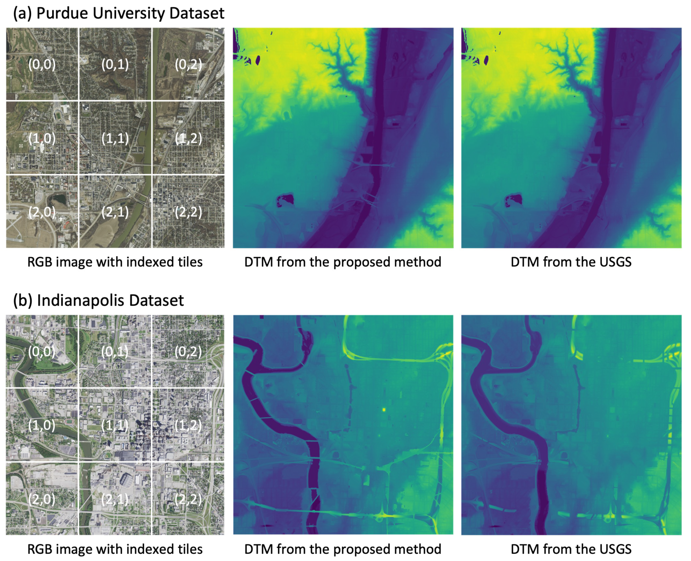
For the micro-analysis, we selected two relatively small (≈20 km2 each) but geographically diverse areas: the Purdue University dataset and the Indianapolis dataset. Figure 4 displays the two datasets, showing their coverage via RGB images with corresponding tile indices, our generated DTMs, and the reference USGS DTMs. We will later use these indexed tiles during the analysis phase in Section 5.1.

Figure 4.
Comparative visualization of the (a) Purdue University and the (b) Indianapolis datasets. Displayed are the RGB images with indexed tiles, the DTMs generated through our method, and the reference DTMs from USGS.
The Purdue University dataset spans the Greater Lafayette area in Indiana, USA and is characterized by a diverse range of landscapes and architectural structures. It includes hilly topographies, rivers, creeks, deep valleys, and a multitude of building types. The diversity of this dataset enables a thorough evaluation of our method across various terrain conditions and structural environments. On the other hand, the Indianapolis dataset covers the center of Indianapolis, the largest city in Indiana. It is characterized by buildings of varied shapes and sizes. This dataset was chosen because it effectively represents the complexities often encountered in typical metropolitan areas. Therefore, it provides a good test case for evaluating the effectiveness of our method in such environments.
The DTM generated by our proposed method, denoted as “OUR”, was benchmarked against five other DTMs originating from different methods. These include three variants based on local neighborhood (slope)-based approaches, namely, “LAS” [20], the progressive morphological filter (“PMF”) [21], and the simple morphological filter (“SMRF”) [26]. The LAS method, developed and implemented through LASTools, employs TIN approximation of the ground. The “PMF” and “SMRF”, are morphological filtering-based methods, proposed in the respective studies [21,26] and were implemented using PDAL [54]. We tested various parameter combinations to find optimal values for each dataset. In addition, we compared our model with the cloth simulation filtering approach (“CSF”) proposed by the study [35]. For the Purdue University dataset, we used the “relief” scenario in CloudCompare, while the “flat” scenario was adopted for the Indianapolis dataset. These methods were selected based on their performance, free availability, and widespread use in large-area terrain modeling projects [11,17,18,42]. Lastly, a DTM provided by the USGS (“USGS”), created by contracted surveying companies using commercial software and proprietary methods with guaranteed quality control, was used as a reference. Recognizing that a single statistic for the entire area might not provide a comprehensive evaluation of different methods, we introduced a tile-based assessment. The DTM was divided into small tiles, each measuring 1.5-km by 1.5-km. For each tile, we computed the mean absolute error (MAE) and root mean square error (RMSE) between each different DTM and the USGS DTM. By doing so, we effectively increased the number of samples, thereby ensuring the results were less affected by outliers and more statistically robust.
For the macro-analysis, we selected four different large-area datasets (≈2400 km2 in total). These datasets include three metropolitan areas and one coastal area: Orlando, FL; Hollywood, FL; Dallas, TX; and Denver, CO, all in the USA. Considering the vastness of these datasets, we benchmarked our method against the USGS DTM. To ensure a more rigorous assessment, we employed a tile-based evaluation approach similar to the micro-analysis. We partitioned the DTM into small 2.5-km by 2.5-km tiles and calculated the tile-wise MAE between our DTM and the USGS DTM.
Lastly, for the parameter analysis, we examined the impact of the slope threshold parameter () using the Boulder dataset where extremely steep mountains and flat urban areas coexist. All airborne LiDAR data were obtained from the USGS’s 3D elevation program (3DEP). We generated all DTMs with a 0.5-m resolution, considering the overall point density of the airborne LiDAR dataset we used.
5. Experimental Results and Discussion
5.1. Micro-Analysis
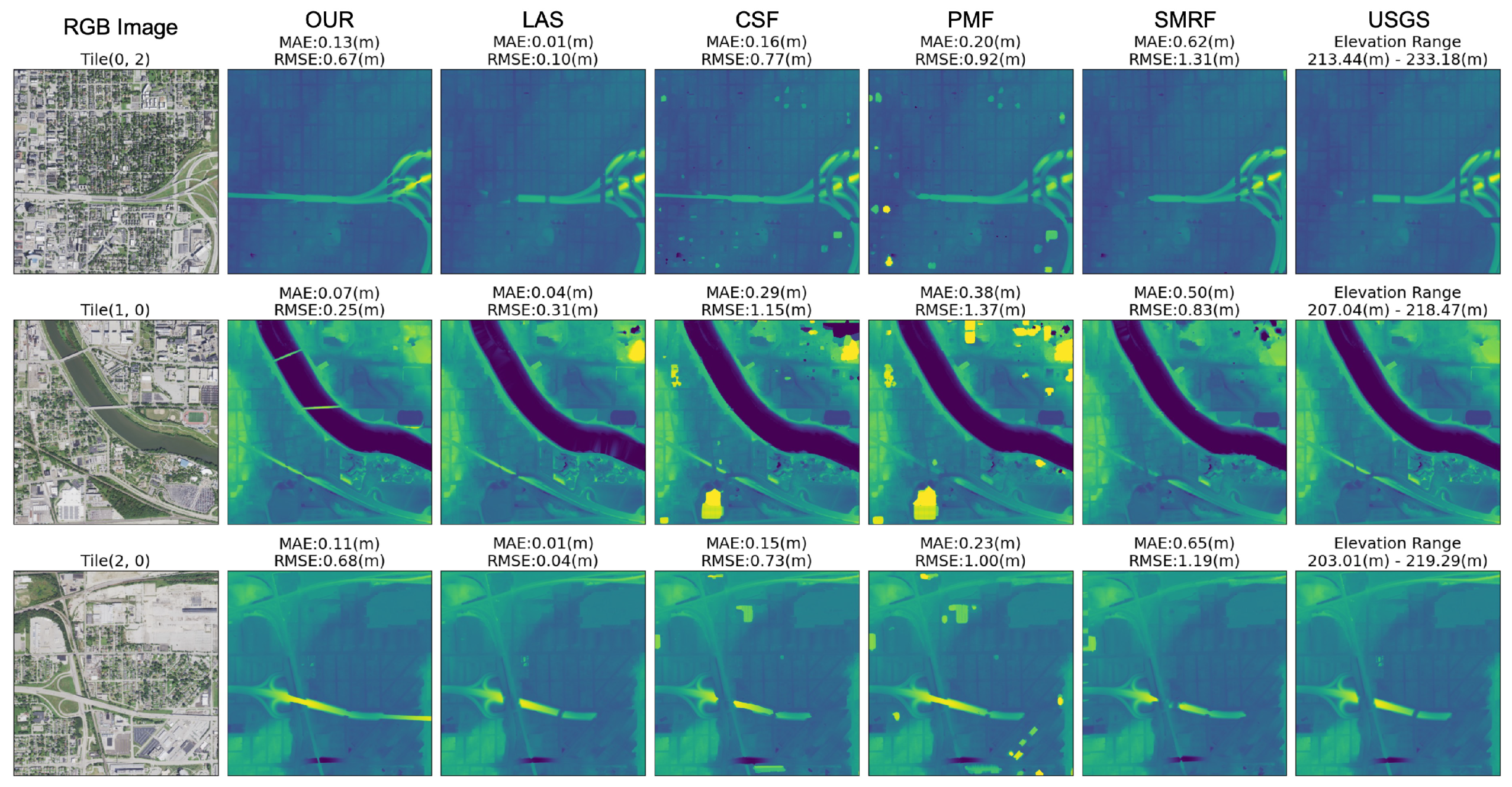
Figure 5 and Figure 6 display DTMs generated by six different methods, along with their corresponding RGB images for three tiles selected from both the Purdue University dataset and the Indianapolis dataset. You can reference the tile indices in Figure 4. The MAE and RMSE are also provided, relative to the USGS’s DTM. Some DTMs produced artifacts near and over water bodies as some methods are not specifically designed to accurately delineate water bodies and their adjacent terrains. Usually, such issues are addressed in subsequent post-processing steps. Here, instead of applying post-processing, we simply excluded the pixels of water bodies and any pixels exhibiting an MAE greater than 10 m in comparison to the USGS’s DTM. This approach helped prevent errors over and near water bodies, as well as certain outliers, from skewing the overall error metrics.
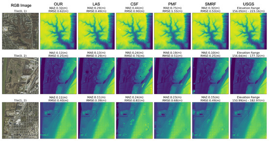
Figure 5.
Comparison of DTMs from different methods for the Purdue University dataset, featuring three representative tiles. Each tile shows its corresponding MAE and RMSE values compared to the USGS’s DTM. The figure shows the reliable performance of our method in geographically complex areas without parameter tunings, particularly noting its superior ability in accurately handling large buildings.

Figure 6.
Comparison of DTMs generated by various methods for the Indianapolis dataset. The figure displays three representative tiles, each with their corresponding MAE and RMSE values when compared to the USGS’s DTM. The figure showcases the robustness of our method in complex urban scenarios, and its outstanding capability in maintaining consistent and unique behavior in terrain modeling, unparalleled by other methods.
As demonstrated in the first row of Figure 5, all DTMs tend to have high RMSEs and MAEs in rugged mountainous areas with deep valleys. In these challenging terrain conditions, our method exhibits performance comparable to other methods. The second row displays areas with relatively flat terrains, where all methods perform reasonably well, with an MAE of less than 0.2 m, except for the CSF, which struggles with filtering one large building. In the third row, all DTMs, with the exception of the DTM derived from our proposed method and the USGS DTM, displayed limited performance in filtering large buildings, with some portions of buildings remaining after ground filtering. Another significant point is that our method, unlike any other methods, treats the entire overpasses as ground, a detail further elaborated upon in Figure 7.
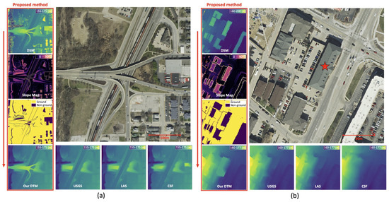
Figure 7.
Notable distinctions of the proposed method: (a) our DTM consistently treats overpasses as ground, in contrast to other methods that show inconsistency; (b) our DTM uniquely identifies an above-ground parking lot adjacent to the building with a red star as ground, attributed to its smooth connection with the access road in the DSM. In contrast, other DTMs classify it as non-ground.
In the first row of Figure 6, an area covering overpasses is displayed. Our method considers the entire overpass as ground since it is smoothly connected to the terrain, while all other methods show the inconsistent mapping of these features. When compared to the USGS’s DTM, which does not categorize overpasses as terrain, our method shows higher error metrics compared to LAS. However, our method yields better results in terms of consistency. The second row displays instances where DTMs from other methods produce artifacts when filtering large objects, whereas our method robustly filters out large buildings. The third row indicates that our method robustly filters buildings of various shapes and sizes while maintaining consistency in overpasses. In contrast, other methods display inconsistency and noise in large building filtering.
Figure 7 zooms into two notable instances observed in the micro-analysis dataset. In Figure 7a, our DTM considers overpasses as ground, while all other DTMs remove only some portions of overpasses, showing inconsistency. In Figure 7b, please note a ground-parking lot of the building marked with a red star. Our DTM recognizes the parking lot as ground, while other DTMs consider it as non-ground. This unique identification is due to the smooth connection between the parking lot and the ground via the access road in the DSM. Although instances like this are rare, it serves as an illustrative example of how our method’s distinguishing attributes can influence the formation of different terrain shapes, diverging from conventional methods.
Overall, the proposed method displays consistent and robust performance in generating DTMs, particularly excelling in filtering large objects and maintaining consistent behavior in the case of overpasses and bridges. It uniquely considers connected artificial terrains as ground and is robust in filtering large buildings. Though unconventional, this approach ensures consistency, a vital property in “modeling”, and offers a valuable option for DTM users, with advantages in road network mapping and object mapping with airborne LiDAR data. Notably, it performs well across diverse building sizes and shapes without the need for parameter tuning, demonstrating scalability for large-area mapping.
Table 2 and Table 3 present quantitative error metrics in comparison to the USGS’s DTM for each of the tiles indexed in Figure 4. Among all methods, LAS shows the lowest errors, followed closely by our proposed method. It should be noted that our method is somewhat disadvantaged in these quantitative metrics as it treats overpasses and bridges as ground, while the reference DTM (USGS’s DTM) does not. Although we tried to obtain reliable performance through multiple trial and errors of parameter combination for other methods, we acknowledge that other methods might have yielded lower errors if more extensive parameter searching was conducted. Nevertheless, considering the fact that we adhered to the default parameter values for our method for the entirety of the dataset, our method is scalable and reliable. Also, the primary standing out point of our method among other many existing methods resides in its unique treatment of overpasses and bridges, and its robustness in filtering large buildings, aspects not paralleled by other methods.

Table 2.
Quantitative comparison of error metrics for the Purdue University dataset.

Table 3.
Quantitative comparison of error metrics for the Indianapolis dataset.
5.2. Macro-Analysis
The main goal of the macro analysis is to thoroughly identify any unexpected artifacts from the proposed method. Using extensive datasets, we compared our DTM to the USGS’s DTM without parameter tuning. The tile-based evaluation was conducted for effective investigation. This method involved: (1) dividing both our method’s and USGS’s DTMs into 2.5-km by 2.5-km tiles; (2) calculating the MAE for each tile pair, considering USGS’s DTMs as a reference; and (3) investigating the tile pair with the largest MAE value. This strategy allowed us to effectively observe the potential artifacts, evaluate the performance objectively, and provide more detailed MAE statistics.
Figure 8 displays the MAE statistics for four macro-analysis datasets. The histograms show tile-based MAE distributions. Most tiles (83% of 370 tiles) had MAEs below 0.15 (m), and average MAEs for the datasets ranged from 0.06 to 0.12 (m). Considering the USGS’s requirements, 0.10 (m) for non-vegetated areas and 0.15 (m) for vegetated areas [55], these results show that our method can produce DTMs with comparable accuracy to USGS requirements without any parameter tuning. Among the entire tiles, we selected the tile that recorded the largest MAE for each dataset and investigated the error sources of the proposed method more in-depth.
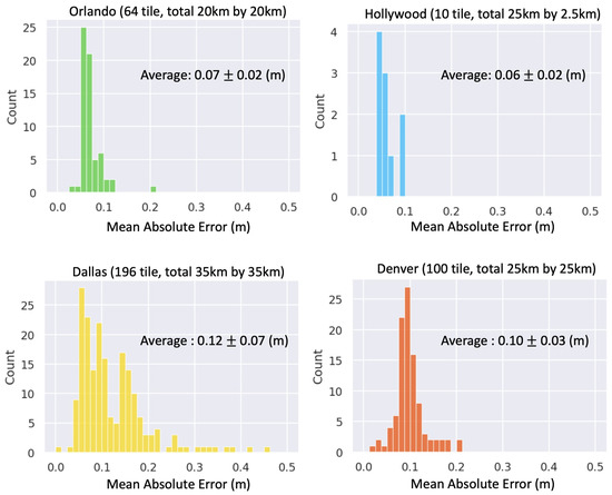
Figure 8.
Mean absolute error (MAE) statistics for the macro-analysis datasets.
Figure 9 displays results from the Orlando dataset, covering the metropolitan area with flat terrain, making artificial objects the main error source. The DTM generated from our method and the USGS’s DTM are shown in Figure 9b,c. Figure 9d–f highlight the largest MAE between our DTM and USGS’s DTM in the dataset. The overpass difference was distinctive, while other differences were minimal. Figure 9g–j, shows zoomed-in images of the orange box delineated in the second row. USGS’s DTM showed significant inconsistency, while our DTM considered overpasses constantly, which can greatly reduce uncertainties in subsequent modeling procedures.
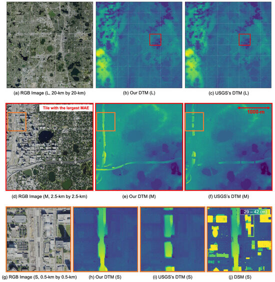
Figure 9.
Results of the Orlando dataset: our method demonstrates consistent behavior for overpasses, unlike the USGS’s DTM, which exhibits inconsistency.
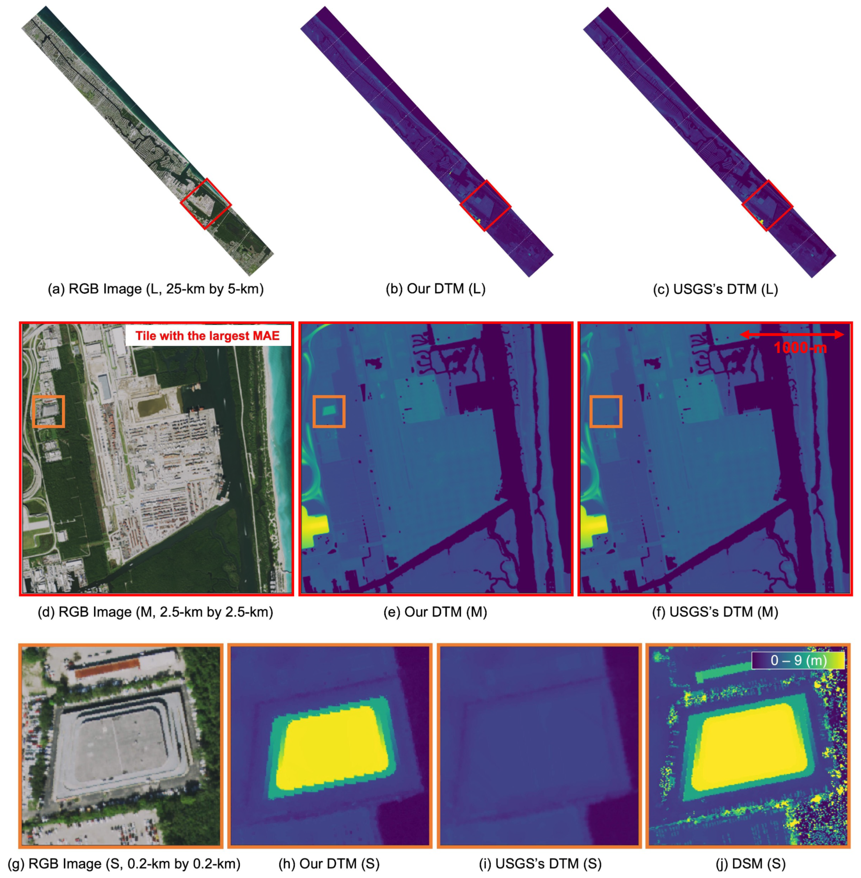
Figure 10 displays results for the Hollywood dataset, a coastal urban area ideal for evaluating the algorithm’s performance. Comparing two DTMs, the proposed method produced hardly any noticeable errors, even without any parameter tuning in terrains adjacent to different types of water bodies. One unique discrepancy was a parking building mapped as terrain due to a smooth connection via a ramp. This is a rare case where our algorithm showed artifacts. Overall, when considering that the USGS’s DTM required a separate hydro-flattening algorithm and manual post-processing for the water body to be the final DTM output, the proposed method, equipped with the water body mapping algorithm, shows a significant advantage in terrain modeling of the coastal urban area as it can automate the whole topographic mapping procedures without requiring any post-processing.
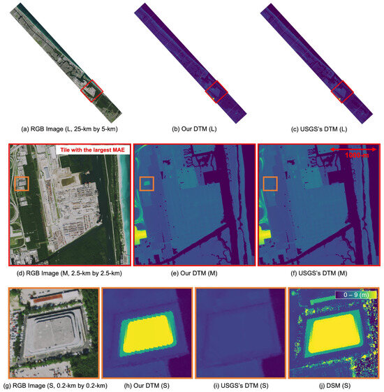
Figure 10.
Results of the Hollywood dataset: only one artifact was found in a unique parking building whose roof is smoothly connected to the first ground floor.
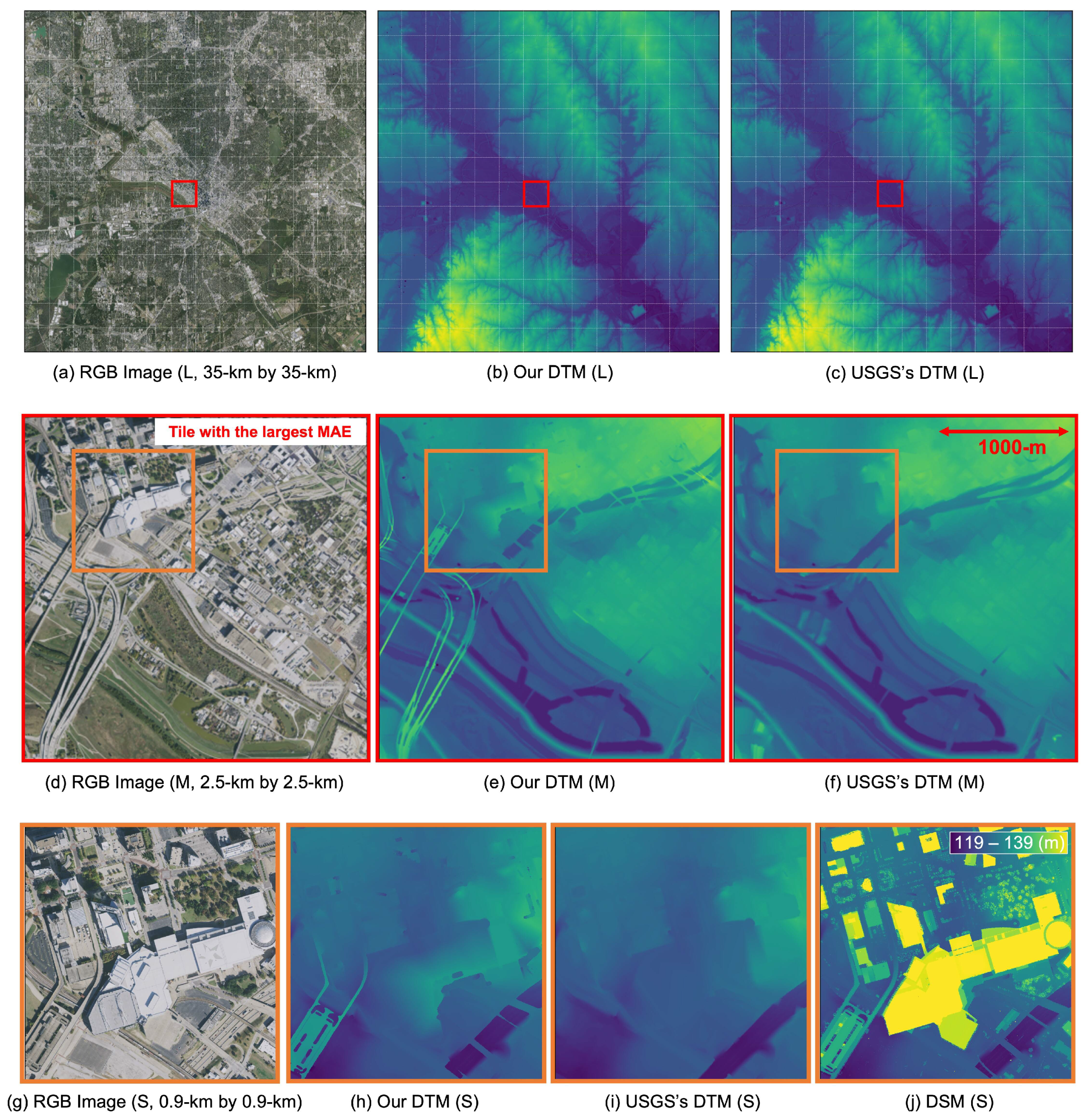
Figure 11 shows the results for the Dallas dataset, an extensive inland metropolitan area in the US. As shown in Figure 11d–f, bridges across a river became a significant portion of the difference. Other than the bridges, only one notable difference was observed in a building whose non-ground floor is connected to the ground by ramps. Except for this building, the proposed method showed better consistency in terrain modeling and produced a DTM very similar to the USGS’s DTM.

Figure 11.
Results of the Dallas dataset: our method is consistent in terms of bridges and overpasses, unlike the USGS’s DTM, but shows an artifact where the building is connected via a ramp.
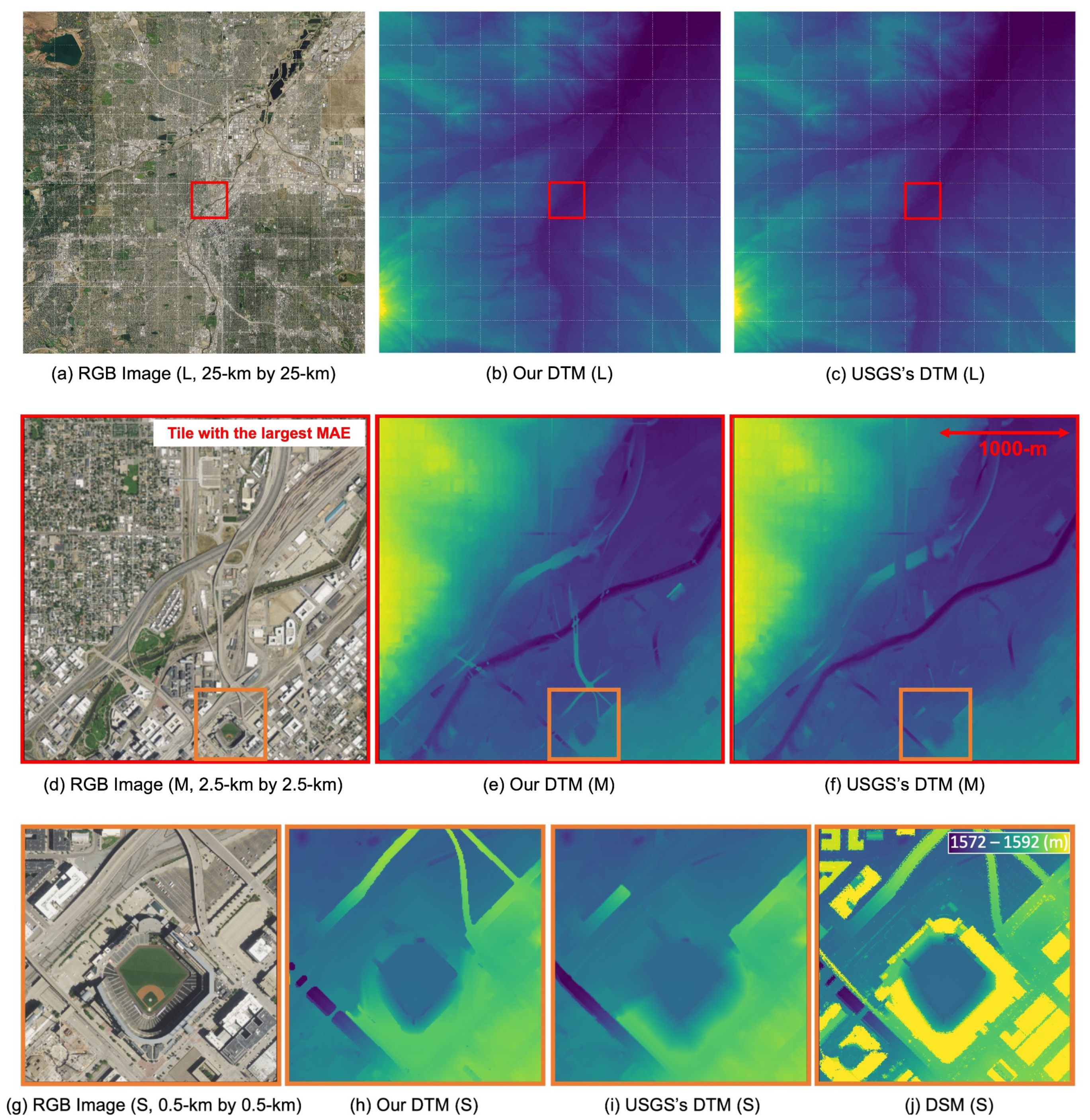
Figure 12 displays the results for the Denver dataset, which encompasses the Denver metropolitan areas and adjacent mountainous regions. Notable differences between the two DTMs were found on overpasses. Figure 12g–j provide zoomed-in images of overpasses and a baseball stadium area. Our DTM consistently considers overpasses as ground, whereas the USGS’s DTM showed inconsistent behavior, breaking the middle of overpasses. Another difference was observed in the baseball stadium. Our method only filtered the built-up part of the stadium as non-ground, while the USGS’s DTM excessively smoothed out the surrounding terrain, losing detailed borders between the object and the original terrain.
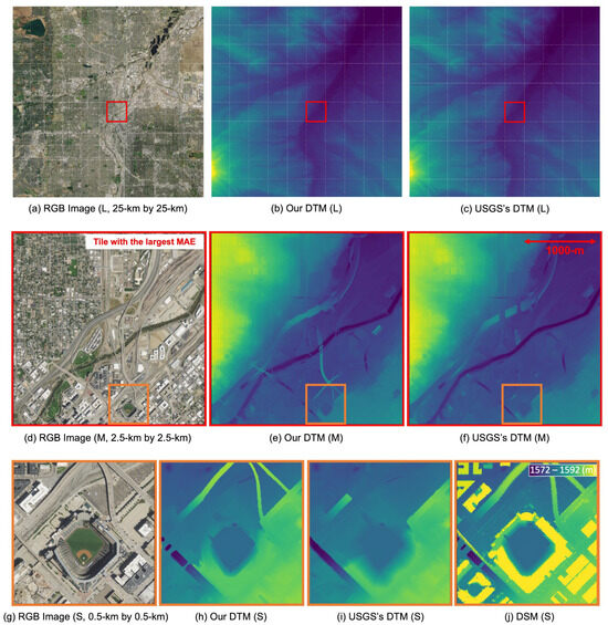
Figure 12.
Results of the Denver dataset: our method shows consistent behaviors in overpasses and precisely delineates the object boundaries without excessively smoothing terrains.
As a result, our method exhibits 0.06–0.12 (m) MAE in varied, extensive experimental areas without parameter tuning, showcasing a satisfactory performance considering the results obtained with a similar type of data as reported in previous studies [42,56]. It is important to note that the MAE reported here was calculated based on a comparison with USGS DTMs, which are generated using different methods employed by USGS contractors. A significant portion of discrepancies can be attributed to differences in DTM properties. In addition, we observed several instances where overpasses were partially classified as ground in USGS DTMs, suggesting that errors can persist in the reference DTM as well, despite the quality control measures implemented by contractors.
We acknowledge that an ideal benchmark would be to compare our results against DTMs generated from carefully and manually classified point clouds. However, such an approach is not feasible due to its labor-intensive requirements, impracticality for large areas, and high costs. Instead, we have employed extensive datasets for a quantitative evaluation of our results and to identify potential artifacts that our method may generate. It is important to remember that the DTM is essentially a model of the terrain and therefore lacks an absolute ground truth. Given this context, our method offers a valuable alternative by providing explicable and consistent results based on a simple rule. We believe the robustness and consistency of our method would faciliate and enhance large-scale terrain modeling projects. Nonetheless, we acknowledge the limitation of not incorporating a point-level classification evaluation and recognize the potential benefits of comparing it against a manually classified point cloud in future studies.
5.3. The Effect of the Slope Threshold
Our method excels in large urban areas, displaying robustness and consistency. However, the default parameter () may need adjustment in very steep mountainous areas as some mountain peaks could be enclosed by the default .
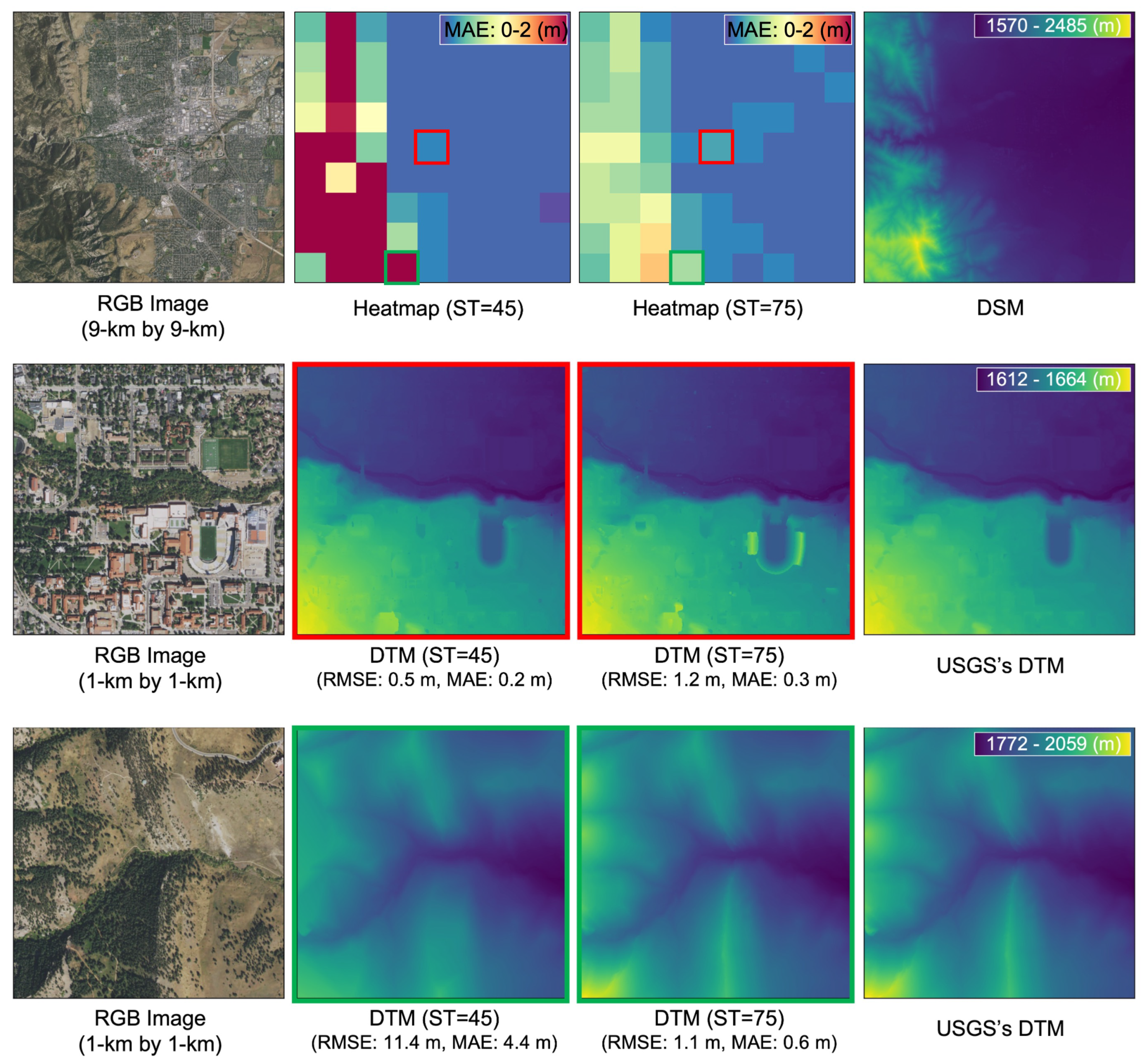
To examine this, we selected the Boulder dataset, covering extremely steep mountain peaks in the Rocky Mountains and a flat urban area, ranging from 1570 (m) to 2485 (m) elevations, making it very difficult to use one single parameter for the entire area.
We created two DTMs with and and compared them to the USGS’s DTM. Like the macro-analysis, we divided the DTM into 1-km by 1-km tiles, calculated tile-based MAEs, and examined error distribution. The first row of Figure 13 shows the aerial RGB image, two heatmaps, and the DSM of the Boulder dataset. The heatmaps at 1 km resolution show the spatial distribution of tile-based MAE between our DTM and the USGS’s DTM. Comparing heatmaps, errors in mountainous areas with decreased with , but urban area MAEs slightly increased with . The second row shows a tile in urban areas. With , the stadium’s upper deck was not filtered as it is connected to lower terrains with slopes less than 75 degrees. The third row displays steep mountainous areas, where smoothed some mountain peaks, while generated steep terrain accurately.
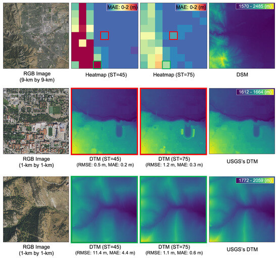
Figure 13.
The effect of the slope threshold: a comparison of the DTM with and the DTM with .
The findings recommend segregating and applying a higher value to areas marked by heavily rugged mountainous terrain. Despite not being free from parameter tuning, our method’s parameter tuning is straightforward, and the results are predictable. This transparency and simplicity enhance user-friendliness and reduce uncertainties in the modeling process, making our approach suitable for large-area terrain modeling, particularly in urban areas.
5.4. Advantages and Limitations
Our object-based ground filtering method provides clear object definition, enhanced scalability, and ease of use for large-area mapping. It is computationally efficient and generates reliable DTMs with minimal parameter tuning, positioning our algorithm as highly effective for large-area DTM modeling.
While our method reduces the need for parameter tuning, it is not entirely exempt from it. Mountainous terrains with peaks may require area division and parameter adjustment. Future research could focus on automatic adaptive tuning. Our method excels in filtering various-sized buildings based on connectivity in the image domain, but it is less suitable for small-area terrain modeling, especially when objects of interest lie on input image boundaries and when ground point classification is the primary goal. This is why our algorithm is less appropriate for point cloud classification within small campaigns (<1 km2, e.g., ISPRS benchmark dataset).
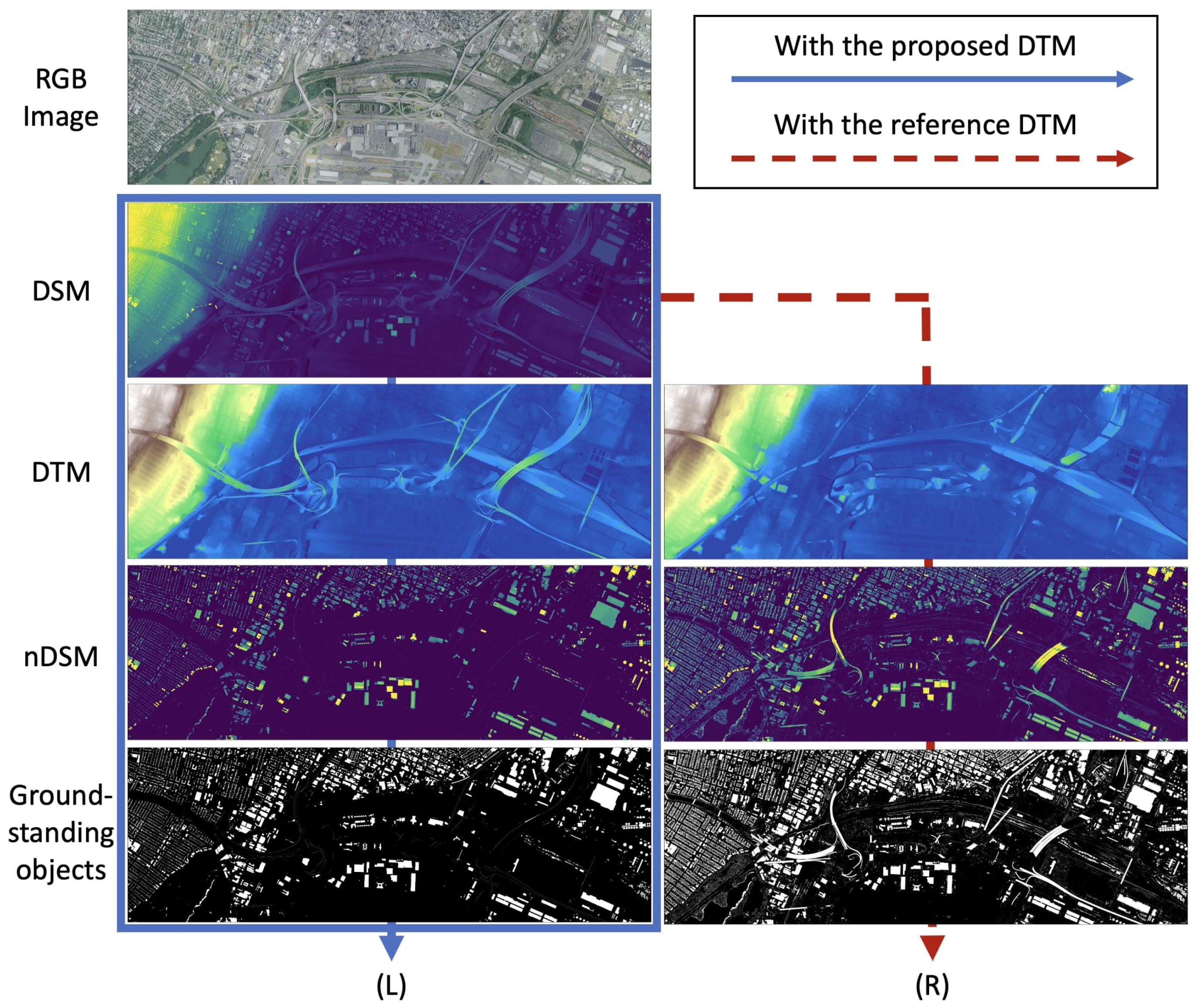
Our method differs from conventional DTM practices as it can include water bodies in the output and modeling process and treats connected artificial terrains as ground. While not always necessary or suitable, these differences facilitate the generation of hydro-flattened DTMs without supplementary optical imagery and benefit object mapping with airborne LiDAR data. As demonstrated in Figure 14, our method results in low nDSM (normalized DSM) values for overpasses and bridges, allowing for the separation of ground-standing objects using height thresholds alone. This approach significantly improves 3D object mapping accuracy and efficiency compared to other DTMs, providing unique advantages and making it a valuable option for various research communities.
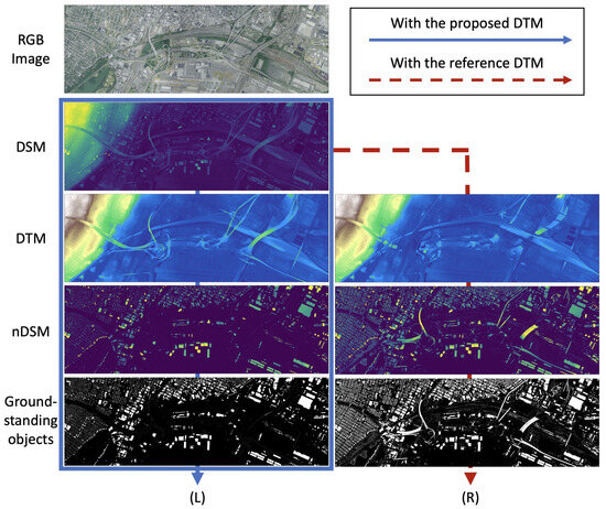
Figure 14.
(L) and (R) depict the exemplary procedures for identifying ground-standing objects using the proposed DTM and the reference DTM, respectively. The reference DTM is sourced from the USGS. The equation is used, with ground-standing objects defined as m. Our method consistently treats bridges and overpasses as ground surfaces, enabling straightforward identification of ground-standing objects. This unique characteristic sets our approach apart from conventional DTMs, offering substantial benefits for 3D urban modeling. (The figure is adapted from [5]; refer to the cited work for more details).
6. Conclusions
We present a new DTM generation method that performs object-based ground filtering. Our method provides a clear definition of objects based on connectivity, allowing for reliable object segmentation and filtering beyond local constraints. The key operation in ground filtering is governed by a single parameter, which delineates the break-line based on slope steepness, and the outcomes of parameter tuning are intuitive and predictable. Unlike other methods, our approach exhibits consistent behavior with connected artificial terrains and presents exclusive features that yield remarkable advantages in applications such as 3D urban modeling and hydro-flattened DTM generation. These findings highlight the potential of our method in delivering reliable DTMs for large-area mapping projects, and the unique features of our method will provide a new valuable addition to existing DTMs for research communities.
Despite these promising results, we acknowledge there are aspects where future work is needed. First, our method’s key filtering operation begins with the DSM, specifically sourced from airborne LiDAR data in our experiments. Considering that our approach can be extended to other sources of airborne point clouds or DSMs, future research could explore applications to DSMs from Structure from Motion (SfM)-generated point clouds from UAV images, DSMs derived from point clouds reconstructed from multi-view satellite images, or DSMs sourced from radar imagery. While our experiments did not cover these aspects, assessing our method’s performance with varying quality of airborne point clouds and DSMs represents an intriguing avenue for future research.
Another consideration involves the evaluation of our method. Although we carried out extensive comparative evaluations and identified potential instances where our method may generate artifacts, the unique behavior of our approach in certain terrains, such as overpasses, prevented us from evaluating it against carefully and manually classified point clouds. However, it is essential to remember that the DTM is essentially a model of the terrain and does not offer an absolute ground truth. Within this context, our method provides a valuable alternative by generating explicable and consistent results based on a simple rule.
We believe the unique, robust, and consistent nature of our method could lead to a new type of DTM, opening avenues for various applications. The code is made available at https://github.com/hunsoosong/object-based-dtm-generation, accessed on 27 June 2023, inviting further examination and improvement.
Author Contributions
Conceptualization and methodology H.S.; writing—original draft preparation, H.S.; writing—review and editing, J.J.; supervision, J.J.; funding acquisition, H.S. and J.J. All authors have read and agreed to the published version of the manuscript.
Funding
This research was funded by the National Geospatial-Intelligence Agency (NGA). Federal Award/Contract No. HM157522D0009/HM157523F0135 (Subaward No. SPC-1000012108/GR132562). Approved for public release, NGA-U-2024-01970.
Data Availability Statement
All LiDAR data used in this study were sourced from the U.S. Geological Survey’s 3D Elevation Program.
Conflicts of Interest
The authors declare no conflict of interest.
Correction Statement
This article has been republished with a minor correction to the Funding statement. This change does not affect the scientific content of the article.
References
- AL-Areeq, A.M.; Sharif, H.O.; Abba, S.; Chowdhury, S.; Al-Suwaiyan, M.; Benaafi, M.; Yassin, M.A.; Aljundi, I.H. Digital elevation model for flood hazards analysis in complex terrain: Case study from Jeddah, Saudi Arabia. Int. J. Appl. Earth Obs. Geoinf. 2023, 119, 103330. [Google Scholar] [CrossRef]
- Pirasteh, S.; Li, J. Developing an algorithm for automated geometric analysis and classification of landslides incorporating LiDAR-derived DEM. Environ. Earth Sci. 2018, 77, 414. [Google Scholar] [CrossRef]
- Samsonov, S.; Blais-Stevens, A. Satellite interferometry for regional assessment of landslide hazard to pipelines in northeastern British Columbia, Canada. Int. J. Appl. Earth Obs. Geoinf. 2023, 118, 103273. [Google Scholar] [CrossRef]
- Song, H.; Jung, J. Challenges in building extraction from airborne LiDAR data: Ground-truth, building boundaries, and evaluation metrics. In Proceedings of the 30th International Conference on Advances in Geographic Information Systems, Seattle, WA, USA, 1–4 November 2022; pp. 1–4. [Google Scholar]
- Song, H.; Jung, J. An unsupervised, open-source workflow for 2D and 3D building mapping from airborne LiDAR data. arXiv 2023, arXiv:2205.14585. [Google Scholar]
- Yan, W.Y.; Shaker, A.; El-Ashmawy, N. Urban land cover classification using airborne LiDAR data: A review. Remote Sens. Environ. 2015, 158, 295–310. [Google Scholar] [CrossRef]
- Qiao, G.; Yuan, X.; Florinsky, I.; Popov, S.; He, Y.; Li, H. Topography reconstruction and evolution analysis of outlet glacier using data from unmanned aerial vehicles in Antarctica. Int. J. Appl. Earth Obs. Geoinf. 2023, 117, 103186. [Google Scholar] [CrossRef]
- Jurado, J.M.; López, A.; Pádua, L.; Sousa, J.J. Remote sensing image fusion on 3D scenarios: A review of applications for agriculture and forestry. Int. J. Appl. Earth Obs. Geoinf. 2022, 112, 102856. [Google Scholar] [CrossRef]
- Osama, N.; Yang, B.; Ma, Y.; Freeshah, M. A Digital Terrain Modeling Method in Urban Areas by the ICESat-2 (Generating precise terrain surface profiles from photon-counting technology). Photogramm. Eng. Remote Sens. 2021, 87, 237–248. [Google Scholar] [CrossRef]
- Sudra, P.; Demarchi, L.; Wierzbicki, G.; Chormański, J. A Comparative Assessment of Multi-Source Generation of Digital Elevation Models for Fluvial Landscapes Characterization and Monitoring. Remote Sens. 2023, 15, 1949. [Google Scholar] [CrossRef]
- Chen, Z.; Gao, B.; Devereux, B. State-of-the-art: DTM generation using airborne LIDAR data. Sensors 2017, 17, 150. [Google Scholar] [CrossRef]
- Uuemaa, E.; Ahi, S.; Montibeller, B.; Muru, M.; Kmoch, A. Vertical accuracy of freely available global digital elevation models (ASTER, AW3D30, MERIT, TanDEM-X, SRTM, and NASADEM). Remote Sens. 2020, 12, 3482. [Google Scholar] [CrossRef]
- Jiménez-Jiménez, S.I.; Ojeda-Bustamante, W.; Marcial-Pablo, M.d.J.; Enciso, J. Digital terrain models generated with low-cost UAV photogrammetry: Methodology and accuracy. ISPRS Int. J. Geo Inf. 2021, 10, 285. [Google Scholar] [CrossRef]
- Zhang, T.; Liu, D. Reconstructing digital terrain models from ArcticDEM and worldview-2 imagery in Livengood, Alaska. Remote Sens. 2023, 15, 2061. [Google Scholar] [CrossRef]
- Bhushan, S.; Shean, D.; Alexandrov, O.; Henderson, S. Automated digital elevation model (DEM) generation from very-high-resolution Planet SkySat triplet stereo and video imagery. ISPRS J. Photogramm. Remote Sens. 2021, 173, 151–165. [Google Scholar] [CrossRef]
- Meng, X.; Currit, N.; Zhao, K. Ground filtering algorithms for airborne LiDAR data: A review of critical issues. Remote Sens. 2010, 2, 833–860. [Google Scholar] [CrossRef]
- Roussel, J.R.; Auty, D.; Coops, N.C.; Tompalski, P.; Goodbody, T.R.; Meador, A.S.; Bourdon, J.F.; De Boissieu, F.; Achim, A. lidR: An R package for analysis of Airborne Laser Scanning (ALS) data. Remote Sens. Environ. 2020, 251, 112061. [Google Scholar] [CrossRef]
- Serifoglu Yilmaz, C.; Yilmaz, V.; Güngör, O. Investigating the performances of commercial and non-commercial software for ground filtering of UAV-based point clouds. Int. J. Remote Sens. 2018, 39, 5016–5042. [Google Scholar] [CrossRef]
- Vosselman, G. Slope based filtering of laser altimetry data. Int. Arch. Photogramm. Remote Sens. 2000, 33, 935–942. [Google Scholar]
- Axelsson, P. DEM generation from laser scanner data using adaptive TIN models. Int. Arch. Photogramm. Remote Sens. 2000, 33, 110–117. [Google Scholar]
- Zhang, K.; Chen, S.C.; Whitman, D.; Shyu, M.L.; Yan, J.; Zhang, C. A progressive morphological filter for removing nonground measurements from airborne LIDAR data. IEEE Trans. Geosci. Remote Sens. 2003, 41, 872–882. [Google Scholar] [CrossRef]
- Chen, Q.; Gong, P.; Baldocchi, D.; Xie, G. Filtering airborne laser scanning data with morphological methods. Photogramm. Eng. Remote Sens. 2007, 73, 175–185. [Google Scholar] [CrossRef]
- Meng, X.; Wang, L.; Silván-Cárdenas, J.L.; Currit, N. A multi-directional ground filtering algorithm for airborne LIDAR. ISPRS J. Photogramm. Remote Sens. 2009, 64, 117–124. [Google Scholar] [CrossRef]
- Chen, Z.; Devereux, B.; Gao, B.; Amable, G. Upward-fusion urban DTM generating method using airborne Lidar data. ISPRS J. Photogramm. Remote Sens. 2012, 72, 121–130. [Google Scholar] [CrossRef]
- Zhang, J.; Lin, X. Filtering airborne LiDAR data by embedding smoothness-constrained segmentation in progressive TIN densification. ISPRS J. Photogramm. Remote Sens. 2013, 81, 44–59. [Google Scholar] [CrossRef]
- Pingel, T.J.; Clarke, K.C.; McBride, W.A. An improved simple morphological filter for the terrain classification of airborne LIDAR data. ISPRS J. Photogramm. Remote Sens. 2013, 77, 21–30. [Google Scholar] [CrossRef]
- Li, Y.; Yong, B.; Wu, H.; An, R.; Xu, H. An improved top-hat filter with sloped brim for extracting ground points from airborne lidar point clouds. Remote Sens. 2014, 6, 12885–12908. [Google Scholar] [CrossRef]
- Hui, Z.; Hu, Y.; Yevenyo, Y.Z.; Yu, X. An improved morphological algorithm for filtering airborne LiDAR point cloud based on multi-level kriging interpolation. Remote Sens. 2016, 8, 35. [Google Scholar] [CrossRef]
- Pijl, A.; Bailly, J.S.; Feurer, D.; El Maaoui, M.A.; Boussema, M.R.; Tarolli, P. TERRA: Terrain extraction from elevation rasters through repetitive anisotropic filtering. Int. J. Appl. Earth Obs. Geoinf. 2020, 84, 101977. [Google Scholar] [CrossRef]
- Li, H.; Ye, C.; Guo, Z.; Wei, R.; Wang, L.; Li, J. A Fast Progressive TIN Densification Filtering Algorithm for Airborne LiDAR Data Using Adjacent Surface Information. IEEE J. Sel. Top. Appl. Earth Obs. Remote Sens. 2021, 14, 12492–12503. [Google Scholar] [CrossRef]
- Chen, C.; Chang, B.; Li, Y.; Shi, B. Filtering airborne LiDAR point clouds based on a scale-irrelevant and terrain-adaptive approach. Measurement 2021, 171, 108756. [Google Scholar] [CrossRef]
- Hui, Z.; Jin, S.; Xia, Y.; Nie, Y.; Xie, X.; Li, N. A mean shift segmentation morphological filter for airborne LiDAR DTM extraction under forest canopy. Opt. Laser Technol. 2021, 136, 106728. [Google Scholar] [CrossRef]
- Kang, C.; Lin, Z.; Wu, S.; Lan, Y.; Geng, C.; Zhang, S. A Triangular Grid Filter Method Based on the Slope Filter. Remote Sens. 2023, 15, 2930. [Google Scholar] [CrossRef]
- Štroner, M.; Urban, R.; Lidmila, M.; Kolář, V.; Křemen, T. Vegetation filtering of a steep rugged terrain: The performance of standard algorithms and a newly proposed workflow on an example of a railway ledge. Remote Sens. 2021, 13, 3050. [Google Scholar] [CrossRef]
- Zhang, W.; Qi, J.; Wan, P.; Wang, H.; Xie, D.; Wang, X.; Yan, G. An easy-to-use airborne LiDAR data filtering method based on cloth simulation. Remote Sens. 2016, 8, 501. [Google Scholar] [CrossRef]
- Li, F.; Zhu, H.; Luo, Z.; Shen, H.; Li, L. An adaptive surface interpolation filter using cloth simulation and relief amplitude for airborne laser scanning data. Remote Sens. 2021, 13, 2938. [Google Scholar] [CrossRef]
- Yilmaz, V. Automated ground filtering of LiDAR and UAS point clouds with metaheuristics. Opt. Laser Technol. 2021, 138, 106890. [Google Scholar] [CrossRef]
- Yu, D.; He, L.; Ye, F.; Jiang, L.; Zhang, C.; Fang, Z.; Liang, Z. Unsupervised ground filtering of airborne-based 3D meshes using a robust cloth simulation. Int. J. Appl. Earth Obs. Geoinf. 2022, 111, 102830. [Google Scholar] [CrossRef]
- Hu, X.; Yuan, Y. Deep-learning-based classification for DTM extraction from ALS point cloud. Remote Sens. 2016, 8, 730. [Google Scholar] [CrossRef]
- Gevaert, C.; Persello, C.; Nex, F.; Vosselman, G. A deep learning approach to DTM extraction from imagery using rule-based training labels. ISPRS J. Photogramm. Remote Sens. 2018, 142, 106–123. [Google Scholar] [CrossRef]
- Li, H.; Ye, W.; Liu, J.; Tan, W.; Pirasteh, S.; Fatholahi, S.N.; Li, J. High-resolution terrain modeling using airborne lidar data with transfer learning. Remote Sens. 2021, 13, 3448. [Google Scholar] [CrossRef]
- Amirkolaee, H.A.; Arefi, H.; Ahmadlou, M.; Raikwar, V. DTM extraction from DSM using a multi-scale DTM fusion strategy based on deep learning. Remote Sens. Environ. 2022, 274, 113014. [Google Scholar] [CrossRef]
- Hu, H.; Zhang, G.; Ao, J.; Wang, C.; Kang, R.; Wu, Y. Multi-information PointNet++ fusion method for DEM construction from airborne LiDAR data. Geocarto Int. 2023, 38, 2153929. [Google Scholar] [CrossRef]
- Song, H.; Kim, Y.; Kim, Y. A patch-based light convolutional neural network for land-cover mapping using Landsat-8 images. Remote Sens. 2019, 11, 114. [Google Scholar] [CrossRef]
- Long, J.; Shelhamer, E.; Darrell, T. Fully convolutional networks for semantic segmentation. In Proceedings of the IEEE Conference on Computer Vision and Pattern Recognition, Boston, MA, USA, 7–12 June 2015; pp. 3431–3440. [Google Scholar]
- Franklin, S.E. Geomorphometric processing of digital elevation models. Comput. Geosci. 1987, 13, 603–609. [Google Scholar] [CrossRef]
- Kanopoulos, N.; Vasanthavada, N.; Baker, R.L. Design of an image edge detection filter using the Sobel operator. IEEE J. Solid State Circuits 1988, 23, 358–367. [Google Scholar] [CrossRef]
- Bolelli, F.; Allegretti, S.; Baraldi, L.; Grana, C. Spaghetti labeling: Directed acyclic graphs for block-based connected components labeling. IEEE Trans. Image Process. 2019, 29, 1999–2012. [Google Scholar] [CrossRef] [PubMed]
- Sithole, G.; Vosselman, G. Experimental comparison of filter algorithms for bare-Earth extraction from airborne laser scanning point clouds. ISPRS J. Photogramm. Remote Sens. 2004, 59, 85–101. [Google Scholar] [CrossRef]
- Song, H.; Jung, J. Scalable surface water mapping up to fine-scale using geometric features of water from topographic airborne LiDAR data. arXiv 2023, arXiv:2301.06567. [Google Scholar]
- Höfle, B.; Vetter, M.; Pfeifer, N.; Mandlburger, G.; Stötter, J. Water surface mapping from airborne laser scanning using signal intensity and elevation data. Earth Surf. Process. Landforms 2009, 34, 1635–1649. [Google Scholar] [CrossRef]
- Heidemann, H.K. Lidar Base Specification; Technical Report; US Geological Survey USGS: Washington, DC, USA, 2012.
- Chen, Z.; Xu, B.; Gao, B. An image-segmentation-based urban DTM generation method using airborne lidar data. IEEE J. Sel. Top. Appl. Earth Obs. Remote Sens. 2016, 9, 496–506. [Google Scholar] [CrossRef]
- PDAL Point Data Abstraction Library. 2022. Available online: https://pdal.io/en/latest/ (accessed on 27 June 2023).
- ASPRS. ASPRS positional accuracy standards for digital geospatial data. Photogramm. Eng. Remote Sens. 2015, 81, A1–A26. [Google Scholar] [CrossRef]
- Kim, M.; Park, S.; Irwin, J.; McCormick, C.; Danielson, J.; Stensaas, G.; Sampath, A.; Bauer, M.; Burgess, M. Positional Accuracy Assessment of Lidar Point Cloud from NAIP/3DEP Pilot Project. Remote Sens. 2020, 12, 1974. [Google Scholar] [CrossRef]
Disclaimer/Publisher’s Note: The statements, opinions and data contained in all publications are solely those of the individual author(s) and contributor(s) and not of MDPI and/or the editor(s). MDPI and/or the editor(s) disclaim responsibility for any injury to people or property resulting from any ideas, methods, instructions or products referred to in the content. |
© 2023 by the authors. Licensee MDPI, Basel, Switzerland. This article is an open access article distributed under the terms and conditions of the Creative Commons Attribution (CC BY) license (https://creativecommons.org/licenses/by/4.0/).

