
Quantitative Characterization of Coastal Cliff Retreat and Landslide Processes at Portonovo–Trave Cliffs (Conero, Ancona, Italy) Using Multi-Source Remote Sensing Data
 , , , , and
Abstract
:1. Introduction
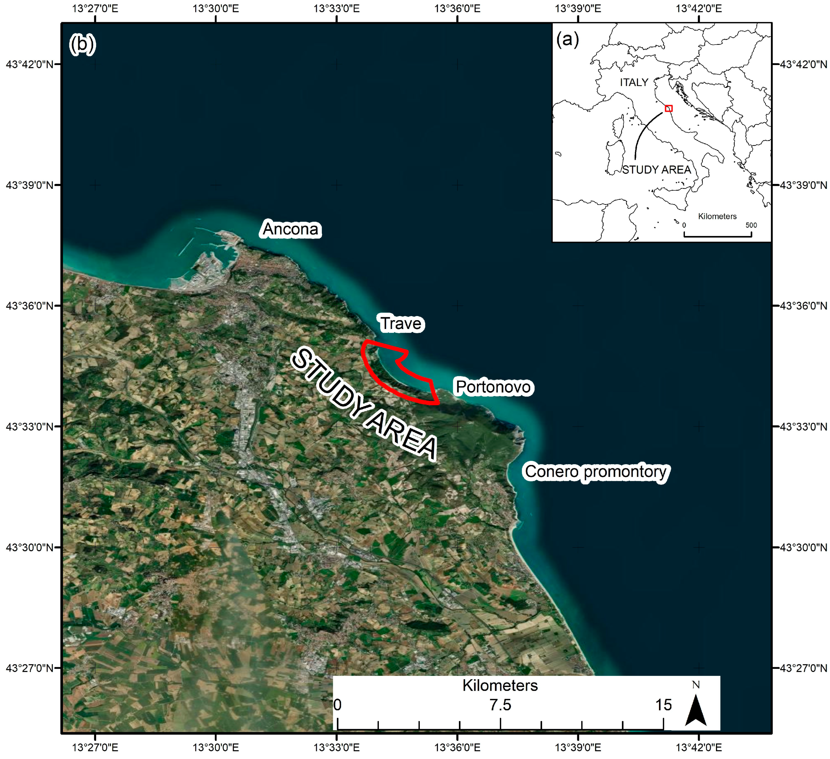
2. Study Area Description
- (a)
- Sector “1”, named Portonovo, is E–O/NW–SE-oriented and stretches from Portonovo to the beginning of the Mezzavalle sector. This sector is mainly characterized by the Schlier Fm.
- (b)
- Sector “2”, called Mezzavalle, is approximately NW–SE-oriented and mainly covered by landslide deposits.
- (c)
- Sector “3”, entitled Trave, approximately N–S/NW–SE-oriented, is characterized by high and steep cliffs (±200 m), along which tectonized flyschoid formations (Argille Azzurre Fm.) outcrop.

3. Materials and Methods
- (a)
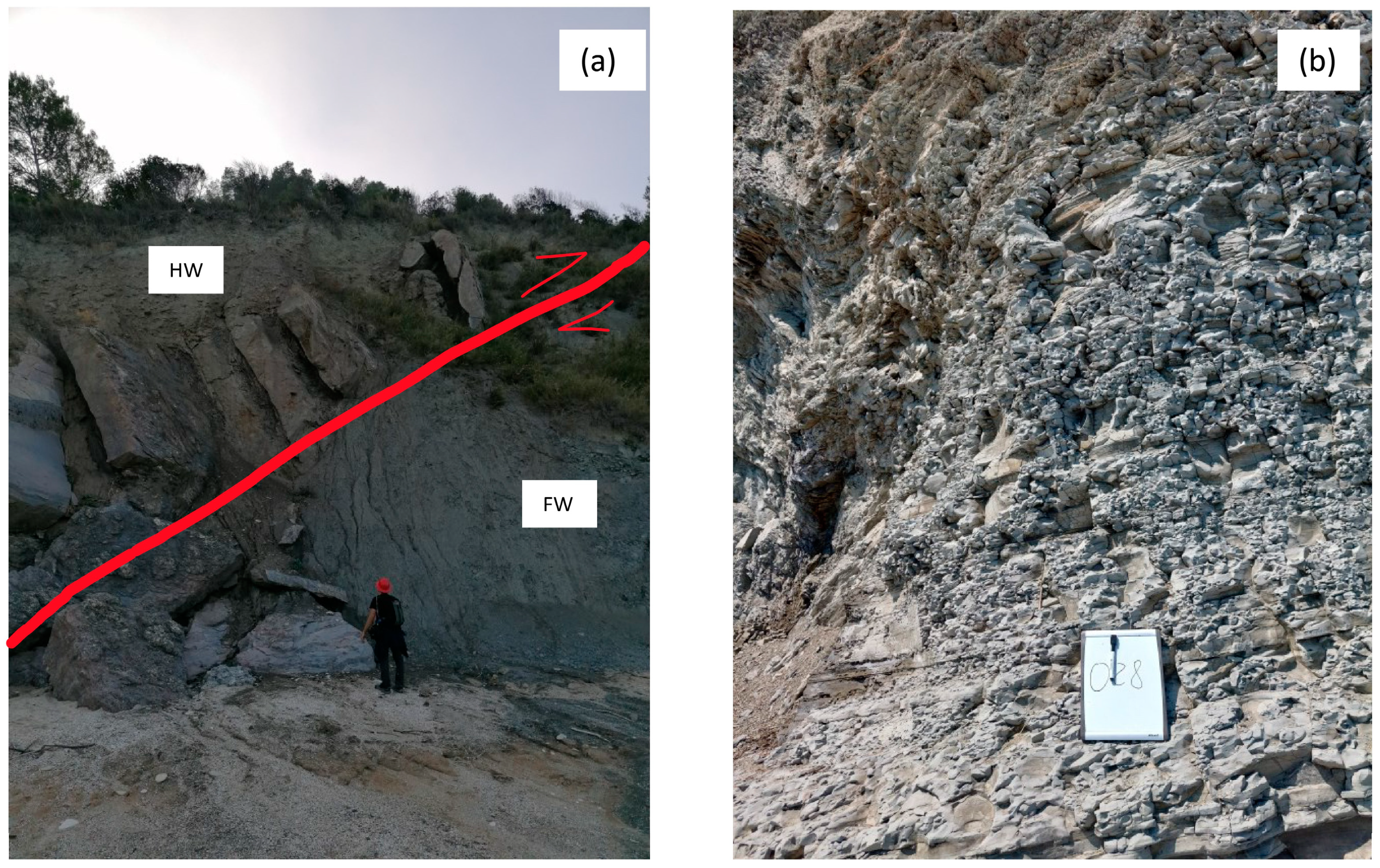
- Fieldwork.
- (b)
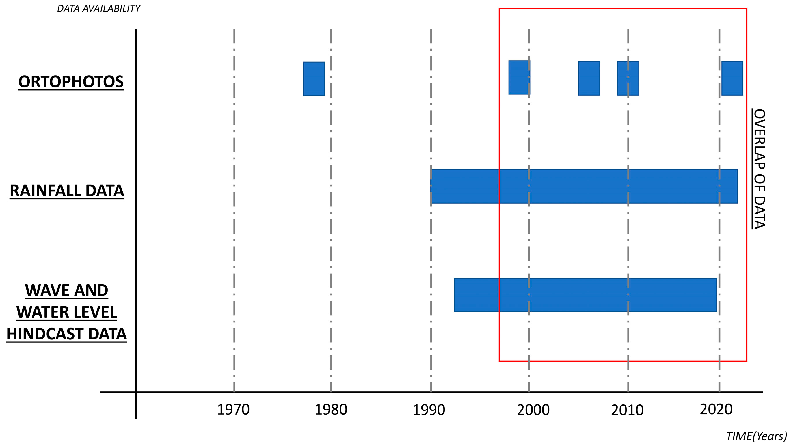
- The analysis of meteorological and marine data.
- (c)
- Cliff-top retreat in different periods, using the DSAS tool for ArcGis. (https://www.arcgis.com/home/index.html (accessed on 24 July 2023)).
- (d)
- DoD between an available 2012 Lidar data and a 2021 DSM extracted from UAV photographs to improve our understanding of cliff-retreat rate and validate results from multitemporal orthoimages analysis.
3.1. Fieldwork and GIS Topographic Analysis
3.2. Analysis of Meteo and Marine Data
3.3. UAV Survey and Data Elaboration
3.4. Morphological Analysis
4. Results
4.1. Fieldwork and GIS Analysis
4.2. Analysis of Meteo and Marine Data
4.3. Morphological Analysis
5. Discussion
6. Conclusions
- (a)
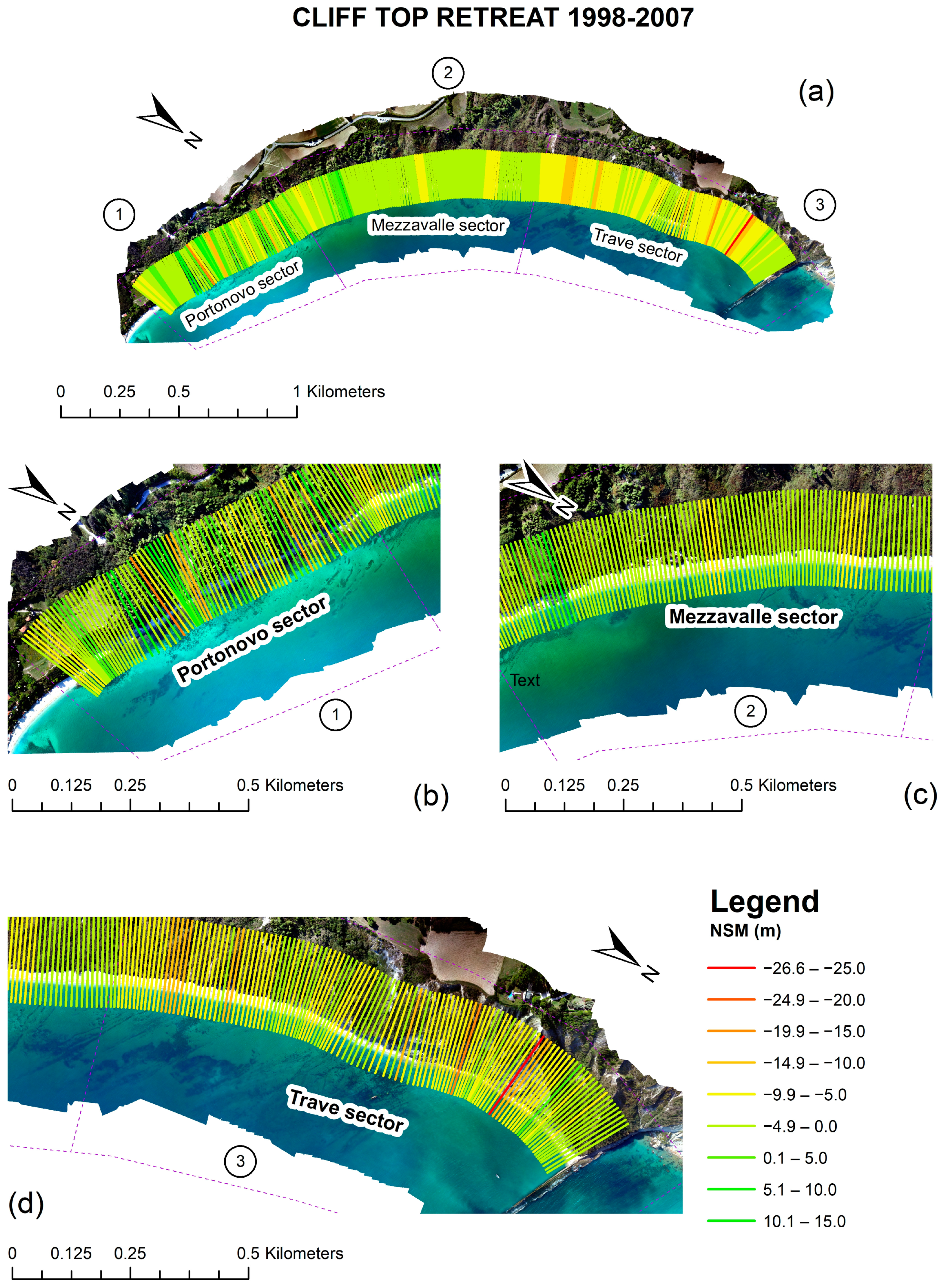
- The coastal area that shows the highest variation in all the time spans considered is the Trave sector, showing an NSM maximum retreat of −43.5 m and a maximum height difference of −31 m.
- (b)
- Comparing different time periods, there is an augmented cliff-top erosion trend over the last 20 years if compared to the whole period of analysis (1978–2021).
- (c)
- The Trave sector shows values of retreat nearly three times higher than the mean value reported in GlobR2C2 [82].
- (a)
- Mechanical properties of the rockmass are decreased due to the presence of tectonic disturbances, which increase fracture intensity and result in a decreasing GSI.
- (b)
- The steepness and elevation of this sector, which is the highest in the entire investigated coastline (both are landslide-predisposing factors).
- (c)
- One of the lowest values of beach width, which increases the role of wave action.
- (d)
- Variations of vegetation rate and land cover may affect the run-off and the erosion in the upper slope.
Author Contributions
Funding
Data Availability Statement
Acknowledgments
Conflicts of Interest
References
- Williams, A.; Pranzini, E. Rock Coasts. In Encyclopedia of Coastal Science; Shwartz, M.L., Ed.; Springer: Berlin/Heidelberg, Germany, 2018. [Google Scholar] [CrossRef]
- Sunamura, T. Rocky Coast Processes: With Special Reference to the Recession of Soft Rock Cliffs. Proc. Japan Acad. Ser. B Phys. Biol. Sci. 2015, 91, 481–500. [Google Scholar] [CrossRef]
- Tsuguo, S. Coastal morphology and research. In Geomorphology of Rocky Coasts; J. Wiley: Chichester, UK; New York, NY, USA, 1992; ISBN 0471917753. [Google Scholar]
- Trenhaile, A.S. Cliffs and Rock Coasts; Elsevier Inc.: Amsterdam, The Netherlands, 2012; Volume 3, ISBN 9780080878850. [Google Scholar]
- Naylor, L.A.; Stephenson, W.J.; Trenhaile, A.S. Rock Coast Geomorphology: Recent Advances and Future Research Directions. Geomorphology 2010, 114, 3–11. [Google Scholar] [CrossRef]
- Brideau, M.A.; Yan, M.; Stead, D. The Role of Tectonic Damage and Brittle Rock Fracture in the Development of Large Rock Slope Failures. Geomorphology 2009, 103, 30–49. [Google Scholar] [CrossRef]
- Piacentini, D.; Troiani, F.; Torre, D.; Menichetti, M. Land-Surface Quantitative Analysis to Investigate the Spatial Distribution of Gravitational Landforms along Rocky Coasts. Remote Sens. 2021, 13, 5012. [Google Scholar] [CrossRef]
- Budetta, P.; Galietta, G.; Santo, A. A Methodology for the Study of the Relation between Coastal Cliff Erosion and the Mechanical Strength of Soils and Rock Masses. Eng. Geol. 2000, 56, 243–256. [Google Scholar] [CrossRef]
- Kennedy, D.M.; Paulik, R.; Dickson, M.E. Subaerial Weathering versus Wave Processes in Shore Platform Development: Reappraising the Old Hat Island Evidence. Earth Surf. Process. Landf. 2011, 36, 686–694. [Google Scholar] [CrossRef]
- Trenhaile, A.S. The Geomorphology of Rock Coasts; Oxford University Press: Oxford, UK, 1987; ISBN 0198232799. [Google Scholar]
- Kennedy, D.M.; Milkins, J. The Formation of Beaches on Shore Platforms in Microtidal Environments. Earth Surf. Process. Landf. 2015, 40, 34–46. [Google Scholar] [CrossRef]
- Komar, P.D.; Shih, S.M. Cliff Erosion along the Oregon Coast: A Tectonic-Sea Level Imprint plus Local Controls by Beach Processes. J. Coast. Res. 1993, 9, 747–765. [Google Scholar]
- Sunamura, T. The Elevation of Shore Platforms: A Laboratory Approach to the Unsolved Problem. J. Geol. 1991, 99, 761–766. [Google Scholar] [CrossRef]
- Robinson, A.H.W. Erosion and Accretion along Part of the Suffolk Coast of East Anglia, England. Mar. Geol. 1980, 37, 133–146. [Google Scholar] [CrossRef]
- Everts, C.H. Seacliff Retreat and Coarse Sediment Yields in Southern California. In Proceedings of the Coastal Sediments ’91 (American Society Civil Engineering), Washington, DC, USA, 25–27 June 1991; pp. 1586–1598. [Google Scholar]
- Poate, T.; Masselink, G.; Austin, M.J.; Dickson, M.; McCall, R. The Role of Bed Roughness in Wave Transformation Across Sloping Rock Shore Platforms. J. Geophys. Res. Earth Surf. 2018, 123, 97–123. [Google Scholar] [CrossRef]
- Prémaillon, M.; Dewez, T.J.B.; Regard, V.; Rosser, N.J.; Carretier, S.; Guillen, L. Conceptual Model of Fracture-Limited Sea Cliff Erosion: Erosion of the Seaward Tilted Flyschs of Socoa, Basque Country, France. Earth Surf. Process. Landf. 2021, 46, 2690–2709. [Google Scholar] [CrossRef]
- Stead, D.; Wolter, A. A Critical Review of Rock Slope Failure Mechanisms: The Importance of Structural Geology. J. Struct. Geol. 2015, 74, 1–23. [Google Scholar] [CrossRef]
- Fazio, N.L.; Perrotti, M.; Andriani, G.F.; Mancini, F.; Rossi, P.; Castagnetti, C.; Lollino, P. A New Methodological Approach to Assess the Stability of Discontinuous Rocky Cliffs Using In-Situ Surveys Supported by UAV-Based Techniques and 3-D Finite Element Model: A Case Study. Eng. Geol. 2019, 260, 105205. [Google Scholar] [CrossRef]
- Brooks, S.; Spencer, T. Storm Impacts on Cliffed Coastlines. In Coastal Storms: Processes and Impacts; Ciavola, P., Coco, G., Eds.; Wiley-Blackwell: Oxford, UK, 2016; ISBN 9781118937099. [Google Scholar]
- Pörtner, H.-O.; Roberts, D.C.; Tignor, M.; Poloczanska, E.S.; Mintenbeck, K.; Alegría, A.; Craig, M.; Langsdorf, S.; Löschke, S.; Möller, V.; et al. IPCC Climate Change 2022: Impacts, Adaptation, and Vulnerability. Contribution of Working Group II to the Sixth Assessment Report of the Intergovernmental Panel on Climate Change; IPCC: Cambridge, UK, 2022. [Google Scholar]
- Bruun, P. Sea-Level Rise as a Cause of Shore Erosion. J. Waterw. Harb. Div. 1962, 88, 117–130. [Google Scholar] [CrossRef]
- Ashton, A.D.; Walkden, M.J.A.; Dickson, M.E. Equilibrium Responses of Cliffed Coasts to Changes in the Rate of Sea Level Rise. Mar. Geol. 2011, 284, 217–229. [Google Scholar] [CrossRef]
- Rosser, N.J.; Petley, D.N.; Lim, M.; Dunning, S.A.; Allison, R.J. Terrestrial Laser Scanning for Monitoring the Process of Hard Rock Coastal Cliff Erosion. Q. J. Eng. Geol. Hydrogeol. 2005, 38, 363–375. [Google Scholar] [CrossRef]
- Matano, F.; Pignalosa, A.; Marino, E.; Esposito, G.; Caccavale, M.; Caputo, T.; Sacchi, M.; Somma, R.; Troise, C.; De Natale, G. Laser Scanning Application for Geostructural Analysis of Tuffaceous Coastal Cliffs: The Case of Punta Epitaffio, Pozzuoli Bay, Italy. Eur. J. Remote Sens. 2015, 48, 615–637. [Google Scholar] [CrossRef]
- Esposito, G.; Matano, F.; Sacchi, M.; Salvini, R. Mechanisms and Frequency-Size Statistics of Failures Characterizing a Coastal Cliff Partially Protected from the Wave Erosive Action. Rend. Lincei 2020, 31, 337–351. [Google Scholar] [CrossRef]
- Caputo, T.; Marino, E.; Matano, F.; Somma, R.; Troise, C.; De Natale, G. Terrestrial Laser Scanning (TLS) Data for the Analysis of Coastal Tuff Cliff Retreat: Application to Coroglio Cliff, Naples, Italy. Ann. Geophys. Geophys. 2018, 61, 110. [Google Scholar] [CrossRef]
- Del Río, L.; Posanski, D.; Gracia, F.J.; Pérez-Romero, A.M. A Comparative Approach of Monitoring Techniques to Assess Erosion Processes on Soft Cliffs. Bull. Eng. Geol. Environ. 2020, 79, 1797–1814. [Google Scholar] [CrossRef]
- Warrick, J.A.; Ritchie, A.C.; Adelman, G.; Adelman, K.; Limber, P.W. New Techniques to Measure Cliff Change from Historical Oblique Aerial Photographs and Structure-from-Motion Photogrammetry. J. Coast. Res. 2017, 33, 39–55. [Google Scholar] [CrossRef]
- Westoby, M.J.; Brasington, J.; Glasser, N.F.; Hambrey, M.J.; Reynolds, J.M. “Structure-from-Motion” Photogrammetry: A Low-Cost, Effective Tool for Geoscience Applications. Geomorphology 2012, 179, 300–314. [Google Scholar] [CrossRef]
- Koukouvelas, I.; Nikolakopoulos, K.G.; Zygouri, V.; Kyriou, A. Post-Seismic Monitoring of Cliff Mass Wasting Using an Unmanned Aerial Vehicle and Field Data at Egremni, Lefkada Island, Greece. Geomorphology 2020, 367, 107306. [Google Scholar] [CrossRef]
- Francioni, M.; Coggan, J.; Eyre, M.; Stead, D. A Combined Field/Remote Sensing Approach for Characterizing Landslide Risk in Coastal Areas. Int. J. Appl. Earth Obs. Geoinf. 2018, 67, 79–95. [Google Scholar] [CrossRef]
- Martino, S.; Mazzanti, P. Integrating Geomechanical Surveys and Remote Sensing for Sea Cliff Slope Stability Analysis: The Mt. Pucci Case Study (Italy). Nat. Hazards Earth Syst. Sci. 2014, 14, 831–848. [Google Scholar] [CrossRef]
- Esposito, G.; Salvini, R.; Matano, F.; Sacchi, M.; Danzi, M.; Somma, R.; Troise, C. Multitemporal Monitoring of a Coastal Landslide through SfM-Derived Point Cloud Comparison. Photogramm. Rec. 2017, 32, 459–479. [Google Scholar] [CrossRef]
- Mateos, R.M.; Azañón, J.M.; Roldán, F.J.; Notti, D.; Pérez-Peña, V.; Galve, J.P.; Pérez-García, J.L.; Colomo, C.M.; Gómez-López, J.M.; Montserrat, O.; et al. The Combined Use of PSInSAR and UAV Photogrammetry Techniques for the Analysis of the Kinematics of a Coastal Landslide Affecting an Urban Area (SE Spain). Landslides 2017, 14, 743–754. [Google Scholar] [CrossRef]
- Calligaro, S.; Sofia, G.; Prosdocimi, M.; Dalla Fontana, G.; Tarolli, P. Terrestrial Laser Scanner Data to Support Coastal Erosion Analysis: The Conero Case Study. Int. Arch. Photogramm. Remote Sens. Spat. Inf. Sci. ISPRS Arch. 2013, 40, 125–129. [Google Scholar] [CrossRef]
- Young, A.P. Decadal-Scale Coastal Cliff Retreat in Southern and Central California. Geomorphology 2018, 300, 164–175. [Google Scholar] [CrossRef]
- Casella, E.; Drechsel, J.; Winter, C.; Benninghoff, M.; Rovere, A. Accuracy of Sand Beach Topography Surveying by Drones and Photogrammetry. Geo-Mar. Lett. 2020, 40, 255–268. [Google Scholar] [CrossRef]
- Turner, I.L.; Harley, M.D.; Drummond, C.D. UAVs for Coastal Surveying. Coast. Eng. 2016, 114, 19–24. [Google Scholar] [CrossRef]
- Seymour, A.C.; Ridge, J.T.; Rodriguez, A.B.; Newton, E.; Dale, J.; Johnston, D.W. Deploying Fixed Wing Unoccupied Aerial Systems (UAS) for Coastal Morphology Assessment and Management. J. Coast. Res. 2018, 34, 704–717. [Google Scholar] [CrossRef]
- Duo, E.; Fabbri, S.; Grottoli, E.; Ciavola, P. Uncertainty of Drone-Derived DEMs and Significance of Detected Morphodynamics in Artificially Scraped Dunes. Remote Sens. 2021, 13, 1823. [Google Scholar] [CrossRef]
- Godfrey, S.; Cooper, J.; Bezombes, F.; Plater, A. Monitoring Coastal Morphology: The Potential of Low-Cost Fixed Array Action Cameras for 3D Reconstruction. Earth Surf. Process. Landf. 2020, 45, 2478–2494. [Google Scholar] [CrossRef]
- Cenci, L.; Disperati, L.; Persichillo, M.G.; Oliveira, E.R.; Alves, F.L.; Phillips, M. Integrating Remote Sensing and GIS Techniques for Monitoring and Modeling Shoreline Evolution to Support Coastal Risk Management. GISci. Remote Sens. 2018, 55, 355–375. [Google Scholar] [CrossRef]
- Colica, E.; Galone, L.; D’Amico, S.; Gauci, A.; Iannucci, R.; Martino, S.; Pistillo, D.; Iregbeyen, P.; Valentino, G. Evaluating Characteristics of an Active Coastal Spreading Area Combining Geophysical Data with Satellite, Aerial, and Unmanned Aerial Vehicles Images. Remote Sens. 2023, 15, 1465. [Google Scholar] [CrossRef]
- Thieler, E.R.; Himmelstoss, E.A.; Zichichi, J.L.; Ergul, A. The Digital Shoreline Analysis System (DSAS) Version 4.0—An ArcGIS Extension for Calculating Shoreline Change; US Geological Survey: Reston, VA, USA, 2009.
- Calamita, F.; Coltorti, M.; Pierucci, P.; Pizzi, A. Evoluzione Strutturale e Morfogenesi Plio- Quaternaria Dell ’ Appennino Umbro- Marchigiano Tra Il Pedappennino Umbro e La. Boll. della Soc. Geol. Ital. 1999, 118, 125–139. [Google Scholar]
- Cello, G.; Coppola, L. Modalità e stili deformativi nell’area anconetana Modalità e Stili Deformativi Nell’area Anconetana. Stud. Geol. Camerti 1989, XI, 37–48. [Google Scholar]
- Coltorti, M.; Nanni, T.; Rainone, M. Il Contributo Delle Scienze Della Terra Nell’ Elaborazione Di Un Piano Paesistico: L’ Esempio Del M. Conero, (Marche). Mem. Soc. Geol. Ital. 1987, 37, 629–642. [Google Scholar]
- Iaccarino, S.M.; Bertini, A.; Di Stefano, A.; Ferraro, L.; Gennari, R.; Grossi, F.; Lirer, F.; Manzi, V.; Menichetti, E.; Lucchi, M.R.; et al. The Trave Section (Monte Dei Corvi, Ancona, Central Italy): An Integrated Paleontological Study of the Messinian Deposits. Stratigraphy 2008, 5, 281–306. [Google Scholar]
- Coltorti, M.; Sarti, M. Note Illustrative Della Carta Geologica d’Italia Alla Scala 1:50.000 “Foglio 293—Osimo”. Progetto CARG: ISPRA, Servizio Geologico d’Italia. 2011. Available online: https://www.isprambiente.gov.it/Media/carg/293_OSIMO/Foglio.html (accessed on 24 July 2023).
- Montanari, A.; Mainiero, M.; Coccioni, R.; Pignocchi, G. Catastrophic Landslide of Medieval Portonovo (Ancona, Italy). Geol. Soc. Am. Bull. 2016, 128, 1660–1678. [Google Scholar] [CrossRef]
- Hungr, O.; Leroueil, S.; Picarelli, L. The Varnes Classification of Landslide Types, an Update. Landslides 2014, 11, 167–194. [Google Scholar] [CrossRef]
- Cruden, D.; Cruden, D.M.; Varnes, D.J. Landslide Types and Processes, Transportation Research Board, U.S. National Academy of Sciences, Special Report. Spec. Rep. Natl. Res. Counc. Transp. Res. Board 1996, 247, 36–57. [Google Scholar]
- Carlo, B.; Gino, C.; de Marco, R.; Federico, S.; Tramontana, M. Caratteri Oceanografici Dell’Adriatico Centro-Settentrionale e Della Costa Marchigiana. Stud. COSTIERI 2021, 30, 7–12. [Google Scholar]
- Acciarri, A.; Bisci, C.; Cantalamessa, G.; Cappucci, S.; Conti, M.; Di Pancrazio, G.; Spagnoli, F.; Valentini, E. Metrics for Short-Term Coastal Characterization, Protection and Planning Decisions of Sentina Natural Reserve, Italy. Ocean Coast. Manag. 2021, 201, 105472. [Google Scholar] [CrossRef]
- Perini, L.; Calabrese, L.; Marco, D.; Valentini, A.; Ciavola, P.; Armaroli, C. Le Mareggiate e Gli Impatti Sulla Costa in Emilia-Romagna 1946–2010; Arpa Emilia-Romagna: Bologna, Italy, 2011; ISBN 88-87854-27-5. [Google Scholar]
- Grottoli, E.; Bertoni, D.; Ciavola, P.; Pozzebon, A. Short Term Displacements of Marked Pebbles in the Swash Zone: Focus on Particle Shape and Size. Mar. Geol. 2015, 367, 143–158. [Google Scholar] [CrossRef]
- Ulusay, R. Rock Characterization Testing and Monitoring. In ISRM Suggested Methods; Springer: Cham, Switzerland, 2015; ISBN 0080273084. [Google Scholar]
- Hoek, E.; Marinos, P.G.; Marinos, V.P. Characterisation and Engineering Properties of Tectonically Undisturbed but Lithologically Varied Sedimentary Rock Masses. Int. J. Rock Mech. Min. Sci. 2005, 42, 277–285. [Google Scholar] [CrossRef]
- Marinos, P.V. New Proposed Gsi Classification Charts for Weak or Complex Rock Masses. Bull. Geol. Soc. Greece 2017, 43, 1248. [Google Scholar] [CrossRef]
- Marinos, P.; Hoek, E. Estimating the Geotechnical Properties of Heterogeneous Rock Masses Such as Flysch. Bull. Eng. Geol. Environ. 2001, 60, 85–92. [Google Scholar] [CrossRef]
- Marinos, P.; Hoek, E. GSI: A Geologically Friendly Tool for Rock Mass Strength Estimation; ISRM International Symposium: Melbourne, Australia, 2000. [Google Scholar]
- Marinos, V.; Marinos, P.; Hoek, E. The Geological Strength Index: Applications and Limitations. Bull. Eng. Geol. Environ. 2005, 64, 55–65. [Google Scholar] [CrossRef]
- Benetazzo, A.; Davison, S.; Barbariol, F.; Mercogliano, P.; Favaretto, C.; Sclavo, M. Correction of ERA5 Wind for Regional Climate Projections of Sea Waves. Water 2022, 14, 1590. [Google Scholar] [CrossRef]
- Gindraux, S.; Boesch, R.; Farinotti, D. Accuracy Assessment of Digital Surface Models from Unmanned Aerial Vehicles’ Imagery on Glaciers. Remote Sens. 2017, 9, 186. [Google Scholar] [CrossRef]
- Brunetta, R.; Duo, E.; Ciavola, P. Evaluating Short-Term Tidal Flat Evolution Through UAV Surveys: A Case Study in the Po Delta (Italy). Remote Sens. 2021, 13, 2322. [Google Scholar] [CrossRef]
- Fabbri, S.; Grottoli, E.; Armaroli, C.; Ciavola, P. Using High-spatial Resolution Uav-derived Data to Evaluate Vegetation and Geomorphological Changes on a Dune Field Involved in a Restoration Endeavour. Remote Sens. 2021, 13, 1987. [Google Scholar] [CrossRef]
- Talavera, L.; Benavente, J.; Del Río, L. UAS Identify and Monitor Unusual Small-Scale Rhythmic Features in the Bay of Cádiz (Spain). Remote Sens. 2021, 13, 1188. [Google Scholar] [CrossRef]
- Hapke, C.; Plant, N. Predicting Coastal Cliff Erosion Using a Bayesian Probabilistic Model. Mar. Geol. 2010, 278, 140–149. [Google Scholar] [CrossRef]
- Gómez-Pazo, A.; Pérez-Alberti, A.; Trenhaile, A. Tracking the Behavior of Rocky Coastal Cliffs in Northwestern Spain. Environ. Earth Sci. 2021, 80, 757. [Google Scholar] [CrossRef]
- Lollino, P.; Pagliarulo, R.; Trizzino, R.; Santaloia, F.; Pisano, L.; Zumpano, V.; Perrotti, M.; Fazio, N.L. Multi-Scale Approach to Analyse the Evolution of Soft Rock Coastal Cliffs and Role of Controlling Factors: A Case Study in South-Eastern Italy. Geomat. Nat. Hazards Risk 2021, 12, 1058–1081. [Google Scholar] [CrossRef]
- Brooks, S.M.; Spencer, T.; Boreham, S. Deriving Mechanisms and Thresholds for Cliff Retreat in Soft-Rock Cliffs under Changing Climates: Rapidly Retreating Cliffs of the Suffolk Coast, UK. Geomorphology 2012, 153–154, 48–60. [Google Scholar] [CrossRef]
- Del Río, L.; Gracia, F.J. Error Determination in the Photogrammetric Assessment of Shoreline Changes. Nat. Hazards 2013, 65, 2385–2397. [Google Scholar] [CrossRef]
- Fletcher, C.; Rooney, J.; Barbee, M.; Lim, S.; Beach, W.P.; Fletchert, C.; Rooneyt, J.; Barbeef, M.; Limf, S.; Richmond, B. Mapping Shoreline Change Using Digital Orthophotogrammetry on Maui, Hawaii. J. Coast. Res. 2003, 38, 106–124. Available online: http://pubs.er.usgs.gov/publication/70025169 (accessed on 24 July 2023).
- Crowell, M.; Leatherman, S.P.; Buckley, M.K. Historical Shoreline Change: Error Analysis and Mapping Accuracy. J. Coast. Res. 1991, 7, 839–852. [Google Scholar]
- Cenci, L.; Disperati, L.; Sousa, L.P.; Phillips, M.; Alves, F.L. Geomatics for Integrated Coastal Zone Management: Multitemporal Shoreline Analysis and Future Regional Perspective for the Portuguese Central Region. J. Coast. Res. 2013, 65, 1349–1354. [Google Scholar] [CrossRef]
- Virdis, S.G.P.; Oggiano, G.; Disperati, L. A Geomatics Approach to Multitemporal Shoreline Analysis in Western Mediterranean: The Case of Platamona-Maritza Beach (Northwest Sardinia, Italy). J. Coast. Res. 2012, 28, 624–640. [Google Scholar] [CrossRef]
- Buchanan, D.H.; Naylor, L.A.; Hurst, M.D.; Stephenson, W.J. Erosion of Rocky Shore Platforms by Block Detachment from Layered Stratigraphy. Earth Surf. Process. Landf. 2020, 45, 1028–1037. [Google Scholar] [CrossRef]
- Williams, R.D. DEMs of Difference. Geomorphol. Tech. 2012, 2, 1–17. [Google Scholar]
- Jaboyedoff, M.; Oppikofer, T.; Abellán, A.; Derron, M.H.; Loye, A.; Metzger, R.; Pedrazzini, A. Use of LIDAR in Landslide Investigations: A Review. Nat. Hazards 2012, 61, 5–28. [Google Scholar] [CrossRef]
- Committee, F.G.D. Others Geospatial Positioning Accuracy Standards. Fed. Geogr. Data Comm. 1998, 3, 1–28. Available online: https://www.fgdc.gov/standards/projects/accuracy/part3/chapter3 (accessed on 24 July 2023).
- Prémaillon, M.; Regard, V.; Dewez, T.J.B.; Auda, Y. GlobR2C2 (Global Recession Rates of Coastal Cliffs): A Global Relational Database to Investigate Coastal Rocky Cliff Erosion Rate Variations. Earth Surf. Dyn. 2018, 6, 651–668. [Google Scholar] [CrossRef]
- Brasington, J.; Langham, J.; Rumsby, B. Methodological Sensitivity of Morphometric Estimates of Coarse Fluvial Sediment Transport. Geomorphology 2003, 53, 299–316. [Google Scholar] [CrossRef]
- Wheaton, J.M.; Brasington, J.; Darby, S.E.; Sear, D.A. Accounting for Uncertainty in DEMs from Repeat Topographic Surveys: Improved Sediment Budgets. Earth Surf. Process. Landf. 2010, 35, 136–156. [Google Scholar] [CrossRef]
- Woodroffe, C.D. Coasts: Form, Process and Evolution; Cambridge University Press: Cambridge, UK, 2002. [Google Scholar]
- Delle Rose, M.; Parise, M. Speleogenesi e Geomorfologia Del Sistema Carsico Delle Grotte Della Poesia Nell’ambito Dell’evoluzione Quaternaria Della Costa Adriatica Salentina. Atti Mem. Comm. Grotte E. Boegan 2005, 40, 153–173. [Google Scholar]
- Miccadei, E.; Mascioli, F.; Ricci, F.; Piacentini, T. Geomorphology of Soft Clastic Rock Coasts in the Mid-Western Adriatic Sea (Abruzzo, Italy). Geomorphology 2019, 324, 72–94. [Google Scholar] [CrossRef]
- Colantoni, P.; Mencucci, D.; Nesci, O. Coastal Processes and Cliff Recession between Gabicce and Pesaro (Northern Adriatic Sea): A Case History. Geomorphology 2004, 62, 257–268. [Google Scholar] [CrossRef]
- Davies, D.S.; Axelrod, E.W.; O’Conner, J.S. Erosion of the North Shore of Long Island; Technical Report; Marine Sciences Research Center; State University of New York; Stony Brook: Stony Brook, NY, USA, 1972; Volume 18, pp. 1–101. [Google Scholar]
- Griggs, G.B.; Savoy, L.E. Living with the California Coast; Duke University Press: Durham, NC, USA, 1985. [Google Scholar]
- Wolters, G.; Müller, G. Effect of Cliff Shape on Internal Stresses and Rock Slope Stability. J. Coast. Res. 2008, 24, 43–50. [Google Scholar] [CrossRef]
- Benumof, B.T.; Griggs, G.B. The Dependence of Seacliff Erosion Rates on Cliff Material Properties and Physical Processes: San Diego County, California. Shore Beach 1999, 67, 29–41. [Google Scholar]
- Moore, L.J.; Benumof, B.T.; Griggs, G.B. Coastal Erosion Hazards in Santa Cruz and San Diego Counties, California. J. Coast. Res. 1999, 28, 121–139. [Google Scholar]
- Brosens, L.; Campforts, B.; Robinet, J.; Vanacker, V.; Opfergelt, S.; Ameijeiras-Mariño, Y.; Minella, J.P.G.; Govers, G. Slope Gradient Controls Soil Thickness and Chemical Weathering in Subtropical Brazil: Understanding Rates and Timescales of Regional Soilscape Evolution Through a Combination of Field Data and Modeling. J. Geophys. Res. Earth Surf. 2020, 125, e2019JF005321. [Google Scholar] [CrossRef]


| Date (yr) | 1978 | 1998 | 2007 | 2010 | 2021 |
|---|---|---|---|---|---|
| Cell size (m) | 1.28 × 1.28 | 1 × 1 | 0.5 × 0.5 | 0.5 × 0.5 | 0.1 × 0.1 |
| GSI (Flysch) | UCS (MPa) | |
|---|---|---|
| PORTONOVO | 50–60 | 30–35 |
| MEZZAVALLE | / | 0.5–5 |
| TRAVE | 15–30 | 5–30 |
| Periods | Portonovo | Mezzavalle | Trave | |||
|---|---|---|---|---|---|---|
| EPR (m/yr) | ECI (m) | EPR (m/yr) | ECI (m) | EPR (m/yr) | ECI (m) | |
| 1978–2021 | −0.20 | 0.16 | 0.09 | 0.16 | −0.25 | 0.16 |
| 1998–2007 | −0.21 | 0.79 | −0.27 | 0.79 | −0.72 | 0.79 |
| 2010–2021 | −0.40 | 0.62 | −0.09 | 0.62 | −0.42 | 0.62 |
Disclaimer/Publisher’s Note: The statements, opinions and data contained in all publications are solely those of the individual author(s) and contributor(s) and not of MDPI and/or the editor(s). MDPI and/or the editor(s) disclaim responsibility for any injury to people or property resulting from any ideas, methods, instructions or products referred to in the content. |
© 2023 by the authors. Licensee MDPI, Basel, Switzerland. This article is an open access article distributed under the terms and conditions of the Creative Commons Attribution (CC BY) license (https://creativecommons.org/licenses/by/4.0/).
Share and Cite
Fullin, N.; Duo, E.; Fabbri, S.; Francioni, M.; Ghirotti, M.; Ciavola, P. Quantitative Characterization of Coastal Cliff Retreat and Landslide Processes at Portonovo–Trave Cliffs (Conero, Ancona, Italy) Using Multi-Source Remote Sensing Data. Remote Sens. 2023, 15, 4120. https://doi.org/10.3390/rs15174120
Fullin N, Duo E, Fabbri S, Francioni M, Ghirotti M, Ciavola P. Quantitative Characterization of Coastal Cliff Retreat and Landslide Processes at Portonovo–Trave Cliffs (Conero, Ancona, Italy) Using Multi-Source Remote Sensing Data. Remote Sensing. 2023; 15(17):4120. https://doi.org/10.3390/rs15174120
Chicago/Turabian StyleFullin, Nicola, Enrico Duo, Stefano Fabbri, Mirko Francioni, Monica Ghirotti, and Paolo Ciavola. 2023. "Quantitative Characterization of Coastal Cliff Retreat and Landslide Processes at Portonovo–Trave Cliffs (Conero, Ancona, Italy) Using Multi-Source Remote Sensing Data" Remote Sensing 15, no. 17: 4120. https://doi.org/10.3390/rs15174120