Satellite Data Reveal Concerns Regarding Mangrove Restoration Efforts in Southern China

Abstract

Mangrove restoration projects are often evaluated based on the increase in mangrove forest (MF) area, but the reliability of this indicator as a measure of successful restoration is questionable. Considering both numerical and quality dimensions, this study assessed mangrove restoration efforts in the Leizhou Peninsula and Beibu Gulf (LP-BG) in China. The hypothesis was that due to the limited social capital investment in mangrove restoration, there exist hierarchical differences in the urgency of mangrove restoration. Time-series Landsat imagery from the Google Earth Engine platform was used to analyze the MF distribution from 2000 to 2020. A resilience indicator, incorporating resistance and adaptive capacity, was constructed to assess MF quality within identified mangrove boundaries. The results revealed an increase in MF area from 6655.87 ha in 2000 to 14,607.93 ha in 2020. However, the majority (79.6%) of MF patches exhibited low resilience (values < 3), with only a minority (51 patches) demonstrating high resilience. Interestingly, MFs within the mangrove reserve displayed higher resilience, but these areas did not exhibit a significant spatial expansion of MFs. These findings highlight the limitation of relying solely on the net growth in the MF area as an indicator of successful restoration. Instead, an ecologically optimal solution is recommended, focusing on expanding conservation boundaries to include remnant MFs outside protected areas, rather than creating new planting areas. This study provides an assessment framework to evaluate the efficiency of mangrove restoration efforts and offers insights for local decision makers to guide future restoration endeavors.

1. Introduction

Mangroves are crucial marine ecosystems that play a significant role in enhancing human welfare, as recognized in the Sustainable Development Goals (SDGs), such as Goal 13 (Climate Action) and Goal 14 (Life Below Water) [1,2]. However, between 1973 and 2000, the total number of MFs in China decreased by 30,199 ha due to the rapid expansion of coastal aquaculture ponds and farmland [3,4]. The degradation of mangrove ecosystems can result in a decline in human welfare [5]. To mitigate these adverse effects, the Chinese central government proposed an ambitious goal of restoring 60,000 ha of MFs [6]. As the implementers, local governments are required to abide by the negotiated restoration goal. However, for local governments, achieving the mangrove restoration goals on time is often a challenge [7,8,9,10].

MF planting is an operable solution for achieving the restoration goals, especially in severely damaged mangrove areas [11]. Planted mangroves can quickly increase the mangrove populations, and they may grow faster in their initial growth stages than natural MFs due to artificial irrigation, fertilization, and management [12]. Therefore, MF planting is a widely used form of mangrove restoration [13]. However, the selection of planting sites is often based on the desire to achieve a centrally defined area or propagule planting targets (i.e., restoration number) rather than survivorship targets [11]. For example, some low-lying areas with good connectivity and less land use ownership conflicts have become priority planting areas, even though these areas are not the best for mangrove restoration [14]. Therefore, a larger number of MFs have been planted in unsuitable environments, where they are exposed to strong stresses such as low temperatures and flooding [15]. Concerns are arising over whether net growth in the MF area can define successful mangrove restoration.

To address these concerns, there is a need to assess the quality of mangrove restoration using indicators that go beyond numerical targets and consider the quality of the restored MFs. Resilience is expected to serve as an important indicator that reflects the quality of mangrove restoration. Successful mangrove restoration often occurs in locations where mangroves are highly resistant to the impacts of disturbances [16]. Assessing the resilience of MFs will inform whether the current spatial configuration is optimal in terms of prioritizing mangrove conservation and will also provide valuable feedback on mangrove restoration for future conservation goals. Previous studies have measured the resilience of MFs through the recovery rate of NDVI values after rapid disturbances (e.g., hurricane damage) using time-series satellite images [17,18,19,20]. However, the resilience definition in these studies is associated with engineering resilience rather than ecological resilience, as is the case in sustainable mangrove management. Therefore, a popular framework to guide the assessment of MF resilience in terms of ecological resilience has not yet been established.

This study proposed a framework for assessing the resilience of MFs. The hypothesis was that due to the limited social capital investment in mangrove restoration, there exist hierarchical differences in the urgency of mangrove restoration. Resilience (the resilience definition adopted in this study is “the ability of a system and its component parts to absorb, accommodate, or recover from the effects of a potentially hazardous event in a timely and efficient manner, including through ensuring the preservation, restoration, or improvement of its essential basic structures and functions”) was portrayed using two indicators in this study: resistance and adaptive capacity. These indicators were quantitatively measured by three parameters: effect size, colonization stability, and growth trend, respectively. The geodatasets relevant to these parameters were obtained using remote sensing images and were selected to build the assessment model in order to assess MF resilience. The Leizhou Peninsula-Beibu Gulf (LP-BG) area in China is a good case study as over 70% of the MFs in China are distributed there [21,22]. The resultant insights gained from this study have the potential to provide valuable information for local decision makers to adjust next-generation mangrove restoration efforts. Moreover, the developed framework will provide a more comprehensive understanding of the success of mangrove restoration efforts and inform future restoration projects that prioritize both numerical and ecological indicators.

2. Materials and Methods

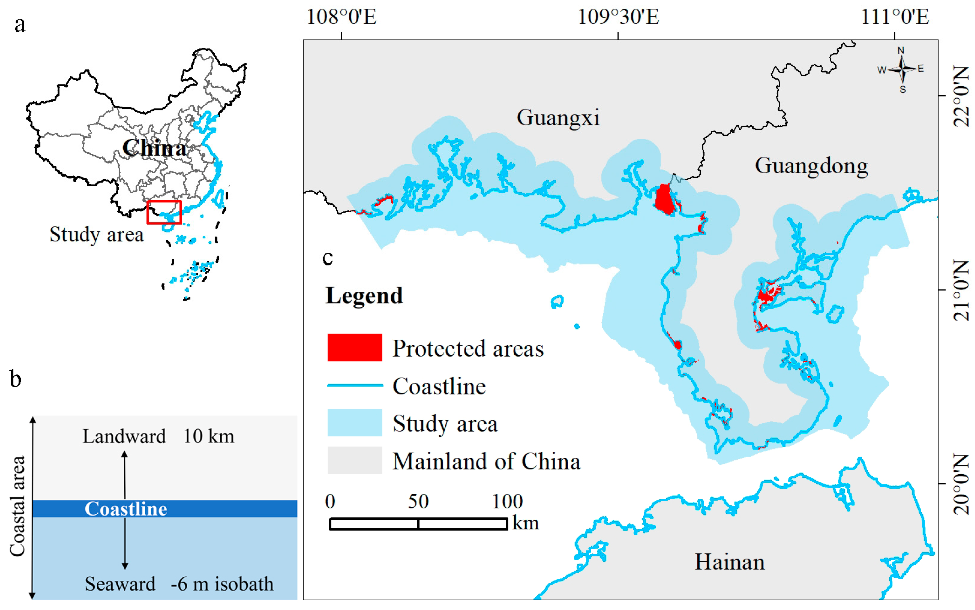
2.1. Study Area

The coastal Leizhou Peninsula-Beibu Gulf (LP-BG) (Figure 1) is a coastal zone located in south of China. Its western part (Beibu Gulf) belongs to Guangxi Province, while the southern and eastern parts (Leizhou Peninsula) belong to Guangdong Province. According to remote sensing-based MF monitoring, 70% of China’s MFs are distributed along the coasts of these provinces [21,22]. The largest mangrove reserve in China, Zhanjiang National Mangrove Nature Reserve, is located in the Leizhou Peninsula and accounts for 33% of the total area of MFs in China. It has been listed by the Ramsar International Convention as an important wetland [23,24]. Moreover, two important mangrove reserves were established in the Beibu Gulf, namely Shankou National Mangrove Natural Reserve and Beilun Estuary National Mangrove Natural Reserve.

The study areas lie within a transitional region spanning subtropical and tropical climates. In the Beibu Gulf, the mean annual temperature is 22.7 °C, and the annual precipitation is 2273.9 mm [25]. Similarly, in the Leizhou Peninsula, the mean annual temperature is 22.3 °C, and the annual precipitation ranges from 1500.0 to 2000.0 mm [24]. The rainy season is concentrated between April and September [26]. Nevertheless, due to the fluctuating monsoon climate, waterlogging and drought frequently occur here [24], and these coastal areas are exposed to a higher risk of sea level rise compared to the world’s mean level [27].

Human activities, such as deforestation and mangrove regulation, have driven fast changes in mangrove distributions in LP-BG. Abundant MF habitats have been replaced by aquaculture and cultivation land since the 1960s because of the higher economic benefits they offer [28]. At the same time, since the 1980s, the mangrove protection policy proposed by the central government of China has provided opportunities for the mangrove ecosystems in LP-BG to receive priority funding support, and half of China’s national mangrove reserves have been situated in the LP-BG [21,29].

2.2. Data Used in This Study

In addition to Landsat satellite images, the auxiliary geospatial data used in this study include a digital elevation model (DEM), released data products about mangrove distribution (

Table A1. Instruction of the released mangrove data products.

Year	Mangrove Data	Source
2000	Hu, et al. and GMF	[52,53]
2005	Hu, et al. and GWM	[53,57]
2010	Hu, et al. and GMF	[52,53]
2015	Hu, et al. and GMF	[52,53]
2020	GWM and GMF	[52,57]

Note: GMF and GMW refer to the thematic mangrove database released by the Global 30-m spatial distribution of mangroves in 2000–2020 and the Global Mangroves Watch, respectively; Hu, et al. refers to the contributor to these mangrove data.

in Appendix D), and Google Earth (GE) images.

Landsat satellites have a series of sensors (TM, ETM+, and OLI/TIRS) to provide optical and thermal images [30]. Most bands for optical images in the Landsat satellite require a spatial resolution of 30 m, and these images can be browsed and accessed in the Google Earth Engine (GEE). The statistics of good observations (less than 40% cloud) from Landsat series images used in this study are presented in Figure A1. Moreover, the digital elevation model (DEM) product used in this study was released by NASA, with a spatial resolution of 30 m, which can be directly browsed and accessed in the GEE and was selected to assist MF mapping. Furthermore, GE images and three released mangrove data products were used for producing validation points to assess the accuracy of MF mapping. Finally, focusing on the area of interest, time-series Landsat images were selected as materials for measuring the indicators in terms of resistance and adaptive capacity, respectively.

2.3. Methodology

RS-based assessments for MF resilience involve answering basic questions, including: (i) Which indicators should be prioritized for inclusion in the model for assessing MF resilience? And (ii) how to depict these indicators via RS technology? A framework for interpreting the methods related to assessing MF resilience is presented in Figure 2. The upper parts of Figure 2 are the workflow for MF mapping, which provides the largest extent of the MF boundary for resilience assessment. The detail workflow for MF resilience assessment are shown in the lower parts of Figure 2.

2.3.1. A Conceptual Resilience Assessment Framework for MFs

Coastal landcover changes (e.g., rapid expansion of coastal aquaculture ponds) along with global changes have put pressure on MFs [31,32]. The impacts of these disturbances on MFs vary due to the spatial differences in MF adaptive capacity. MFs with high adaptive capacity have the high ability to adapt to disturbances. Two parameters, colonization stability and growth trend, were selected to measure the adaptive capacity. Moreover, MFs with high resistance tend to absorb more disturbances, resulting in a smaller effect from disturbances. This parameter is measured by the reduction in MF’s annual NDVI.

2.3.2. Identifying the Largest MF Extent for LP-BG

The purpose of MF mapping in this study was to provide geospatial data for assessing MF resilience. To map MF distributions in LP-BG, a pixel- and phenology-based algorithm was used, which has been previously used in mapping China’s mangroves and coastal evergreen vegetation [22,33,34]. The key features used in this algorithm for identifying MFs include evergreen vegetation and tidal inundation, as MFs are unique, evergreen trees found at estuaries and coasts that are inundated by tides.

The main steps for MF mapping consist of sample collection, identification of MF pixels based on two criteria, frequency estimates of MF pixels, threshold segmentation of frequency, and accuracy assessment for mangrove data product.

• Sample Collection

High-resolution images are used for sample collection. These images provide a geographic coordinate system as well as morphological and spectral information that can assist in sample collection [35,36]. To identify highly reliable areas of MF occurrences, we performed a spatial intersection of several released mangrove data products. The identified mangrove boundaries were then overlaid onto a layer of sub-meter-scale Google Earth (GE) images in a project. Mangrove samples (their geographical locations) were automatically marked on the GE images within these identified mangrove boundaries, as shown in Figure 3.

The polygon-based sampling method used in our study eliminates the influence of outliers, as each mangrove sample (a rectangle with dimensions of 60 m × 60 m) extracts the median value of nine adjacent pixels from a Landsat image. This approach also avoids information redundancy, as adjacent samples with 10-m intervals may appear as independent samples on a submeter image but may be inside the same pixel at an image with a spatial resolution of 30 m. To prevent adjacent mangrove samples from overlapping, we designed a circumscribed box with a size of 100 m. In total, we produced 146 training samples, which were checked using GE images and Landsat time-series images to ensure their locations were inside the mangrove patches during the entire study period. In addition, we used 200 validation samples (including mangrove and non-landcovers) for each phase of the study to assess the accuracy of the mangrove data product.

2.

Identifying the MF Pixels

Three spectral indicators, Enhanced Vegetation Index (EVI), Normalized Difference Vegetation Index (NDVI), and Land Surface Water Index (LSWI), were selected for MF mapping. EVI and NDVI are commonly used indices to identify evergreen vegetation and track its changes [37,38]. LSWI is an important indicator to capture signs of green vegetation and soil moisture, making it useful to identify senescent (dry) vegetation and soils with low moisture [39]. These indicators have been used based on multiple combination criteria to map China’s MFs [33,34].

A histogram analysis of annual mean NDVI, EVI, and LSWI based on training mangrove samples produced by this study indicated that 97% of the MF pixels had EVI values of ≥0.27, NDVI values of ≥0.53, and LSWI values of ≥0.37 (Figure 4). $M_{\mathit{landward}}$, an indicator highlighting vegetation features in relation to MFs, was generated by the criteria of NDVI ≥ 0.53, EVI ≥ 0.27, and LSWI ≥ 0.37, and was used to map MF pixels in this study.

Previous studies have reported that the criteria of LSWI ≥ EVI or LSWI ≥ NDVI can enhance the signals of MFs in low-water areas that are frequently inundated by tides [22]. Therefore, in this study, $M_{\mathit{seaward}},$ an indicator reflecting tidal inundation features in relation to MFs, was generated by the criterion of LSWI ≥ EVI or LSWI ≥ NDVI, which was used to assist in identifying MF pixels.

3.

Frequency Estimates of MF Pixels

Inundation can significantly affect the spectral indicators of MFs, resulting in weaker signals of $M_{\mathit{landward}}$ for frequently inundated MFs and stronger signals of the $M_{\mathit{seaward}}$ indicator. Conversely, rarely inundated MFs tend to have stronger signals of the $M_{\mathit{landward}}$ indicator and weaker signals of $M_{\mathit{seaward}}$. Therefore, using variable frequency thresholds is more appropriate than fixed frequency thresholds from an instantaneous image, as it can help reduce the impacts of tidal inundation and phenology on MF pixels. The frequency of $M_{\mathit{landward}}$ ($F_{\mathit{ML}}$) within a pixel in a year was calculated using Equation (1), and the frequency of $M_{\mathit{seaward}}$ ($F_{\mathit{MS}}$) within a pixel in a year was calculated using Equation (2):

$$F_{\mathit{ML} }=\frac{{N(M}_{\mathit{landward}})}{N_{\mathit{good}}}$$

(1)

$$F_{\mathit{MS}}=\frac{{N(M}_{\mathit{seaward}})}{N_{\mathit{good}}}$$

(2)

where $F_{\mathit{ML}}$ and $F_{\mathit{MS}}$ range from 0% to 100%, ${N(M}_{\mathit{landward}})$ is the number of $M_{\mathit{landward}}$ observations in a year, and $N_{\mathit{good}}$ is the number of valid observations in a year. Similarly, $F_{\mathit{MS}}$ is the ratio of the number of $M_{\mathit{seaward}}$ observations ${N(M}_{\mathit{seaward}})$ over the number of good-quality observations $N_{\mathit{good}}$. Moreover, $F_{\mathit{ML}}$ and $F_{\mathit{MS}}$ are presented in Figure 5b,c.

In order to determine appropriate frequency thresholds for potential MF pixels in high- and low-water areas, we conducted a histogram analysis of $M_{\mathit{landward}}$ and $M_{\mathit{seaward}}$ (Figure A2). Based on the statistical results, we identified rules that could be used to identify pixels in high- and low-water areas as potential MFs, if they meet certain criteria. Note that the mapping algorithm used in this study employs variable frequency thresholds to accurately capture the geographic distribution features of MFs in both high and low-water areas, even in regions with different inundation regimes [22].

Moreover, we applied mask files that included the four geographic parameters (as shown in Figure A3) to filter the potential MF pixels. Areas with steep slopes or high elevations, for instance, are less likely to be MFs, so these areas were excluded from the potential MF pixels. Similarly, areas with high texture values or low yearlong water frequency values were also excluded, as they are unlikely to be MFs. By applying these geographic parameters as filters, the accuracy of MF mapping was significantly enhanced, ensuring that only genuine MF pixels were included in the final output.

4.

Post-classification and Accuracy Assessment

We identified the maximum extents of MFs in the LP-BG using the outer boundaries of all available mangrove data products, which were generated for the years 2000, 2005, 2010, 2015, and 2020. These boundaries were used as the area of interest for assessing the resilience of MFs in LP-BG. Additionally, we calculated the precision of the mangrove data products for each phase using accuracy (Equation (3)) and F1 scores [40,41], as shown in Equations (4)–(6):

$$\mathit{Accuracy}=\frac{T_P+T_N}{T_P+F_P+F_N+T_N}$$

(3)

$$\mathit{Precision}=\frac{T_P}{T_{P }+F_P}$$

(4)

$$\mathit{Recall}=\frac{T_P}{T_{P }+F_P}$$

(5)

$$F_1=2 \times \frac{\mathit{Precision} \times \mathit{Recall}}{\mathit{Precision}+\mathit{Recall}}$$

(6)

where T_P, T_N, F_P, F_N, and N in Equations (3)–(6) represent True Positive, True Negative, False Positive, False Negative, and the total number of items, respectively.

Moreover, in order to ensure the reliability and accuracy of the mangrove data product, we compared the mangrove data product with the historical GE images to identify any discrepancies between the two datasets. This approach allowed us to evaluate the accuracy of the MF mapping algorithm and ensure that the mangrove data produced by GEE were reliable and accurate.

2.3.3. Calculating Resistance Indicator

The resistance of mangroves to environmental variability can provide insight into their resilience to ecological shifts, which is important when measuring responses associated with disturbances [42]. If MF pixels are highly resistant, they can efficiently maintain a stable structure and function in the face of external disturbances. Resistance thus indirectly reflects the potential capacity of MFs to absorb disturbances [43,44,45]. In this study, the resistance indicator was selected to portray one aspect of the resilience of MF pixels. This indicator was determined by quantifying the maximum deviation in the annual NDVI of a measurable MF pixel from the baseline of the time-series NDVI. The LandTrendr algorithm played a crucial role in this step, as it generated trajectory-based time-series NDVI data with minimal inter-annual signal noise.

The LandTrendr algorithm enables the detection of pixel-based resistance to disturbances in the time series of Landsat images [46,47], which is reflected in the dropped magnitude of the annual NDVI inside MF pixels [48]. The higher the dropped magnitude of annual NDVI, the smaller the resistance of MF pixels. Moreover, based on the previous literature [49], the output from LandTrendr (the largest drop in magnitude of annual NDVI inside the pixels during the study periods) was reclassified into four ranks (

Table 1. Grade division of the dropped magnitude of annual NDVI.

Description of the Dropped Magnitude of NDVI	Threshold Intervals	Rank	Description of Resistance
Not significant	0.00 ≤ ΔNDVI < 0.02	1	Strong
Slight	0.02 ≤ ΔNDVI < 0.15	2	High
Moderate	0.15 ≤ ΔNDVI < 0.35	3	Middle
Severe	ΔNDVI ≥ 0.35	4	Low

Note: Research of Chen, et al., (2020) [49] provides criteria for threshold division.

). The higher the rank, the smaller the resistance of MF pixels. By using this approach, the resistance of MF pixels to disturbances can be quantified and integrated into the assessment of MF resilience.

2.3.4. Calculating Adaptive Capacity Indicator

Adaptive capacity is the ability of a system to adjust and respond to changes in its environment. In this study, two parameters, growth trend and colonization stability, were selected to portray the adaptive capacity indicator of MFs. MFs with a better growth trend and higher colonization stability tend to have higher adaptive capacity.

The growth trend of the MFs inside the patches was quantified by the slope values of the time-series fractional vegetation cover (FVC) [50,51]. The slope values of FVC were categorized into three ranks (

Table 2. Grade division for growth trend.

Quartile	Threshold Ranges	Rank	Description of Growth Trend
0~25%	−0.06 ≤ ΔFVC < 0.00	1	Descend
25~75%	0.00 ≤ ΔFVC < 0.03	2	Steady
75~100%	0.03 ≤ ΔFVC < 0.07	3	Ascend

) using the quartile interval method in ArcGIS 10.5. Higher slope values of FVC indicate more favorable trends in the adaptive capacity of the mangrove canopy. This approach enables the quantification of growth trends and the integration of these data into the assessment of the MFs’ adaptive capacity.

Colonization stability was quantified by the frequency of the MF attribute within a pixel using the five-period mangrove data products produced by this study. The colonization stability ranks ranged from 1 to 5, where higher colonization stability ranks corresponded to higher adaptive capacity (

Table 3. Grade division for colonization stability.

The Frequency of Occurrence of MF Attributes within a Pixel	Rank	Description of Colonization Stability
1	1	weak
2	2	low
3	3	middle
4	4	high
5	5	strong

).

Finally, the adaptive capacity was calculated based on the growth trend and colonization stability using Equation (7). The value of adaptive capacity ranged from 1 to 15, with higher values indicating greater adaptive capacity of the MFs. This approach allowed for the quantification of the adaptive capacity of MF pixels by integrating both growth trends and colonization stability.

$${\mathit{adaptive} \mathit{capacity}}_{\mathit{ij}}={\mathit{growth} \mathit{trend}}_{\mathit{ij}}{\times \mathit{colonization} \mathit{stability}}_{\mathit{ij}}$$

(7)

where ${\mathit{adaptive} \mathit{capacity}}_{\mathit{ij}}$, ${\mathit{growth} \mathit{trend}}_{\mathit{ij}}$, and ${\mathit{colonization} \mathit{stability}}_{\mathit{ij}}$ are pixel values in the i-th row and j-th column of their corresponding raster.

2.3.5. Resilience Assessment for MFs

This study constructed a function based on the resistance indicator and adaptive capacity indicator to calculate the resilience of MFs. The constructed function can be expressed as follows (8):

$$\mathit{resilience}=f (\mathit{resistance}, \mathit{adaptive} \mathit{capacity})$$

(8)

A higher resilience value represents a higher MF resilience. Specifically, based on the multiplication rule, this study calculated the resilience of MFs using the following Equation (9):

$${\mathit{resilience}}_{\mathit{ij} }{=1/\mathit{resistance}}_{\mathit{ij}}{\times \mathit{adaptive} \mathit{capacity}}_{\mathit{ij}}$$

(9)

where ${\mathit{resilience}}_{\mathit{ij}}$, ${\mathit{resistance}}_{\mathit{ij}}$, and ${\mathit{adaptive} \mathit{capacity}}_{\mathit{ij}}$ are pixel values in the i-th row and j-th column of their corresponding raster. Using the ArcGIS 10.5, the resilience value is calculated based on Equation (9), and the normalized resilience values are divided into five equidistant levels.

This equation allowed for the integration of both the resistance and adaptive capacity indicators into the assessment of MF resilience. By multiplying the two indicators, the function provided a quantitative measure of the resilience of MF pixels. The higher the resilience value, the greater the ability of the MF pixels to absorb and adapt to disturbances. Note that in this study, the resilience ranking of MFs is based on a relative ranking system, and this system compares the resilience of different MF pixels within the study area rather than delivering an absolute measure of resilience.

The mean resilience value of pixels within each MF patch was calculated using Equation (10):

$$B_k=\frac{\sum P_{\mathit{ij}}}{n}$$

(10)

where $B_k$ represents the $k$th mangrove landscape patch, $P_{ij}$ represents the pixel values of resilience in j-th column i-th row within the MF landscape patch, and $n$ represents the total number of pixels within a patch.

3. Results

3.1. Spatial Distribution of the Largest MF Extent for LP-BG

The total number of MFs in the LP-BG increased from 6655.87 ha in 2000 to 14,607.93 ha in 2020, with a sharply increasing trend over the study period. Moreover, the mangrove distribution displays a substantial spatial heterogeneity (Figure 6). MFs are more abundant along the east coast than the west coast in terms of longitude. Hotspots of MFs are mainly located in the inner bay, such as Maowei Sea, Dafeng River, Lianzhou Bay, and the east coast of Leizhou Peninsula. Notably, the highest number of MFs was observed in Tongming Sea. Along the latitude direction, mangroves are abundant in the high latitudes of the LP-BG, while they exhibit sporadic distribution in the southern part of the Leizhou Peninsula.

3.2. Spatial Pattern of Resistance and Adaptive Capacity

3.2.1. Spatial Pattern of Resistance

The majority of MFs in the LP-BG are highly resistant to disturbances (Figure 7). The statistics show that 80.91% of MFs are classified as having a high resistance (rank 1), while only 4.21% of MFs are identified as having a low resistance (rank 4).

Resistance in ranks 1 and 2 is observed in most MF patches. In mode a, resistance in ranks 3 4 is sporadically distributed within the core area of the MF patches. In mode b, resistance in rank 4 is displayed throughout the entire MF patch, particularly in the Maowei Sea area. In modes c and d, resistance in ranks 3 and 4 is sporadically distributed in the low-tide area (nascent MF area). In mode e, resistance in rank 4 is sporadically distributed adjacent to the coastlines.

3.2.2. Spatial Pattern of Adaptive Capacity

Based on the statistics provided, it appears that the majority (80.06%) of MFs in the study period showed a rising trend in their vegetation coverage (Figure A4). However, only 15.42% of MFs had a strong colonization stability throughout the study period (Figure A5).

The adaptive capacity of MFs varies across different regions, with those within the mangrove reserve (Figure 8e) exhibiting higher adaptive capacity compared to those in other coastal areas, which is attributed to their strong growth trend and colonization stability. Interestingly, certain MF patches with robust colonization stability experience a low trend in vegetation coverage, resulting in lower adaptive capacity (Figure 8c). Additionally, the edges of MF patches adjacent to the coastline (high water) often exhibit lower adaptive capacity.

Adaptive capacity in ranks 1–2 is primarily observed at the edges of the MF patches adjacent to high-tide areas. In modes b and c, adaptive capacity in ranks 3–5 is mainly observed within the core area of the MF patches, while in modes d and e, these ranks are also observed at the edges of the MF patches. Adaptive capacity in ranks 6–15 is mainly observed in the protected areas, and it can also be observed in the core areas of the MF patches in modes a and c.

3.3. Resilience of MFs in the LP-BG

According to the statistics, MFs with weak resilience only account for 0.1%, but the majority (77.64%) of MFs show low and middle resilience. The resilience of the MFs varied across different areas in the LP-BG, with those within the mangrove reserve (Figure 9e) showing higher resilience than those in other coastal areas. However, the edge of the MF patches was often exposed to lower resilience.

Resilience in rank 1 occupies the entire MF patches in mode b, while it is sporadically distributed in other modes. Resilience in rank 2 is observed in the majority of the area in mode d. Resilience in ranks 3–5, characterized by a mosaic structure, is observed in modes a, c, and the protected area.

The statistical analysis of the mean resilience values within MF patches indicates an overall inadequate level of MF resilience. Out of the total number of patches, only a limited subset (56) exhibited a resilience value ≥ 3, while the majority (79.6%) had a value < 3. Interestingly, larger MF patches demonstrated higher resilience compared to fragmented ones, while small MF patches adjacent to aquaculture ponds and rivers generally displayed lower resilience (Figure 10c). Additionally, MF patches with a naturally expanding mode exhibited higher resilience compared to artificially planted MF patches (Figure 10d). Furthermore, the MF patches within the reserve showed higher resilience values compared to those observed in the surrounding areas (Figure 10e).

4. Discussion

4.1. Comparison with Other Available MF Maps

Our results indicate a rapid increase in the number of mangroves in the LP-BG, as shown in

Table 4. Statistics of the mangrove data and their precision between 2000 and 2020.

Year	This Study (ha)	Hu, et al. (ha)	GMF (ha)	GWM (ha)	Accuracy (This Study)	F1 Score (This Study)
2000	6655.87	6613.65	4988.37	—	0.89	0.83
2005	8871.15	8144.46	—	14,285.05	0.91	0.86
2010	11,240.30	10,500.39	7246.79	13,133.06	0.92	0.88
2015	11,579.10	12,459.42	11,500.39	14,065.93	0.93	0.90
2020	14,607.93	—	11,695.54	13,505.12	0.93	0.89
2000–2020	17,256.78	—	—	—	—	—

Note: GMF and GMW refer to the thematic mangrove database released by the Global 30-m spatial distribution of mangroves in 2000–2020 and Global Mangroves Watch, respectively; Hu, et al. refers to the contributor to these mangrove data. The GWM data in 2005 are unavailable and have been substituted with data from 2007 in this dataset.

. This conclusion is consistent with other mangrove data products, such as GMF’s version [52] and Hu et al.’s version [53], but it has not been confirmed by global mangrove data products such as GWM’s version. The mangrove numbers in our study are very similar to those in Hu et al.’s version and slightly higher than those in GMF’s version, as shown in Figure 11. However, the mangrove numbers in GWM’s version differ significantly from our data products. These differences may be due to smaller mapping errors in our study compared to other mangrove products. As shown in Figure 11, the mangrove data produced in our study closely match the MF areas on GE images. In contrast, other mangrove data products are largely missing in low-tide areas, and GMW’s version notably occupies many pixels without mangrove properties, resulting in falsely high mangrove numbers on land. These findings provide qualitative evidence of the high quality of MF mapping in our study.

Overall, our findings indicate that the MF mapping algorithm employed in our study is characterized by high accuracy and reliability, making it valuable for informing conservation and restoration initiatives. The divergences observed between our data products and other mangrove datasets underscore the significance of utilizing robust mapping algorithms and conducting cross-validation with additional datasets to ensure the precision and dependability of mangrove data.

4.2. Area Increasing Does Not Reflect That Mangrove Restoration Is Succeeding Sufficiently

Our study revealed a significant increase in the MF area in the LP-BG, from 6655.87 ha in 2000 to 14,607.93 ha in 2020. However, our analysis also indicated that the majority (79.6%) of MF patches exhibited low resilience (values < 3), primarily in newly established areas (Figure 10). In contrast, a minority of MF patches (51 patches) showed strong resilience and were mainly located within the mangrove reserve. However, these areas did not exhibit a significant spatial expansion of MFs. Additionally, our observations indicated that successful mangrove restoration often takes decades, and mangroves in the seedling stage and growth period are particularly vulnerable. Some mature MFs with long lifespans also suffered significant degradation due to the invasion of spartina alterniflora, as observed in hotspots in Dandou Bay (Figure 12c). Therefore, although there is a general upward trend in MF coverage, failing to consider mangrove quality may result in an underestimation of the systemic risk associated with MF sub-health. It may be premature to draw conclusions about the complete success of mangrove restoration efforts, particularly when considering resilience as an assessment criterion.

The lessons learned from mangrove restoration management in Southeast Asian countries, such as the Philippines, echo our assessment. In order to achieve the negotiated conservation numbers, most MF plantations only plant a single mangrove species, and other MF species are often artificially removed. As a result, MFs in these plantations have high densities, short and narrow canopies, and few species [54]. Compared to natural MFs, these MF characteristics are not conducive to the stability of mangrove ecosystems. The vigilant lesson learned from the Philippines informs us that an increase in the area of MFs does not reflect successful mangrove restoration efforts. Therefore, the evaluation framework constructed in this study can provide a tool for evaluating the effectiveness of restoration efforts in global mangrove hotspots.

In conclusion, assessing the success of mangrove restoration efforts based solely on the MF area indicator is insufficient. A comprehensive assessment should also consider quality factors such as resilience. By considering both the quantity and quality of MFs, we can better understand the effectiveness of mangrove restoration efforts and develop more informed conservation and management strategies.

4.3. Priority Solutions for Mangrove Restoration

The selection of mangrove restoration methods is strongly influenced by the assessment methods used to evaluate the effectiveness of mangrove restoration work. Monitoring the increase in mangrove numbers is often chosen as the primary criterion for assessing the success of restoration efforts in large-scale regions due to its strong operability [55,56]. However, in natural-based mangrove restoration, it typically takes decades to significantly improve the fitness of mangroves, making it difficult to achieve rapid restoration at large scales through natural recovery alone. In contrast, planting mangroves can significantly increase the area of mangroves in a short time, which provides a quick way to achieve the desired quantity restoration targets. In many cases, local governments are often under pressure to complete restoration goals within a short period of time, which leads to the prioritization of quantity-based restoration measures. However, this emphasis on quantity can lead to poor site and single species selection, which in turn increases the systemic risk associated with MF sub-health. If large-scale planting becomes the primary solution to complete the assessment task, it will weaken natural recovery and may mislead future restoration policies, ultimately increasing the risk of degradation.

Therefore, instead of focusing solely on quantity-based restoration measures, it is important to consider the quality of MFs. Extending the protection of all existing mangroves may be the optimal option for nature-based mangrove restoration. Our studies show that the resilience of mangroves in protected areas is higher than outside of them. Given that most mangroves are in their infancy stage and not sufficiently adaptable to changing environments, incorporating all existing mangroves into the scope of protection can provide a stable environment for mangrove seedlings to enter the mature stage smoothly. Additionally, targeted MF planting can assist in areas where mangrove degradation is severe and natural restoration is difficult to achieve. These measures are expected to help achieve the goals of mangrove restoration in a sustainable manner.

In conclusion, while monitoring the increase in mangrove numbers is a useful assessment method, it should not be the sole criterion for evaluating the effectiveness of mangrove restoration efforts. A comprehensive approach that considers both quantity and quality factors is needed to develop effective and sustainable mangrove restoration strategies.

4.4. Strengths and Weakness of This Study

A pixel- and phenology-based algorithm was utilized to map the mangrove distributions in the study area. The classification of MFs was based on time-series Landsat imagery, which greatly reduced misclassification typically caused by the effects of tidal inundation on vegetation indices. This algorithm improved the visibility of mangrove features on the images, resulting in a highly accurate mangrove data product that provided basic data for assessing the resilience of MFs. Furthermore, the resilience indicators used in this study were constructed based on two indicators: resistance and adaptive capacity. These indicators portrayed the mangrove features in multiple dimensions, allowing for a more comprehensive assessment of mangrove restoration compared to a single area-based indicator. The synergistic effect of multiple parameters can effectively assess mangrove restoration and provide valuable insights for future restoration efforts.

However, the quality of the input image data may introduce uncertainty in the assessment results. In tropical coastal areas with mangrove distributions, cloud cover can be abundant, and the spatial inconsistency of good-quality observations may still cause some uncertainties in the resultant mangrove data products. Additionally, mixed pixels of evergreen vegetation and water can affect the annual maps of MFs, particularly when certain MFs exhibit very low $F_{\mathit{ML}}$ values in a specific year.

Moreover, the resilience assessment for MFs is based on a relative ranking system that compares the resilience of different MFs, rather than delivering an absolute measure of resilience. Therefore, some MFs that have gone extinct are still assigned a resilience rank of non-significant. However, in practical settings, it is important to consider the resilience of MFs that are not above their adaptive capacity threshold.

5. Conclusions

We used a pixel- and phenology-based algorithm to map the spatial distributions of MFs in the LP-GB. We found a consistent increase in the number of MFs in the LP-BG, expanding from 6655.87 ha in 2000 to 14,607.93 ha in 2020. However, a resilience indicator constructed for assessing the quality of MFs revealed that the majority (79.6%) of MF patches exhibited low resilience (values < 3), predominantly in newly established MF areas. Interestingly, MFs within the mangrove reserve displayed higher resilience, but these areas did not exhibit a significant spatial expansion of MFs. Consequently, we cannot use the net growth in an MF area to define successful mangrove restoration in the study area, and it may be premature to conclude that mangrove restoration efforts have been fully successful. Furthermore, we recommend an ecologically optimal solution for mangrove restoration, which is to include the remnant MFs outside the current protected areas within the conservation scope. The framework related to the resilience assessment of MFs proposed in this study is flexible and can serve as a paradigm for other mangrove hotspots.

References

1. Sasmito, S.D.; Basyuni, M.; Kridalaksana, A.; Saragi-Sasmito, M.F.; Lovelock, C.E.; Murdiyarso, D. Challenges and opportunities for achieving Sustainable Development Goals through restoration of Indonesia’s mangroves. Nat. Ecol. Evol. 2023, 7, 62–70. [Google Scholar] [CrossRef]
2. Chow, J. Mangrove management for climate change adaptation and sustainable development in coastal zones. J. Sustain. For. 2018, 37, 139–156. [Google Scholar] [CrossRef]
3. Jia, M.; Wang, Z.; Mao, D.; Huang, C.; Lu, C. Spatial-temporal changes of China’s mangrove forests over the past 50 years: An analysis towards the Sustainable Development Goals (SDGs). Chin. Sci. Bull. 2021, 66, 3886–3901. [Google Scholar] [CrossRef]
4. Meng, X.W.; Xia, P.; Li, Z.; Meng, D.Z. Mangrove degradation and response to anthropogenic disturbance in the Maowei Sea (SW China) since 1926 AD: Mangrove-derived OM and pollen. Org. Geochem. 2016, 98, 166–175. [Google Scholar] [CrossRef]
5. Barbier, E.B.; Strand, I.; Sathirathai, S. Do open access conditions affect the valuation of an externality? Estimating the welfare effects of mangrove-fishery linkages in Thailand. Environ. Resour. Econ. 2002, 21, 343–367. [Google Scholar] [CrossRef]
6. Fan, H.; Wang, W. Some Thematic Issues for Mangrove Conservation in China. J. Xiamen Univ. Nat. Sci. 2017, 56, 323–330. [Google Scholar]
7. Veas-Ayala, N.; Alfaro-Cordoba, M.; Quesada-Roman, A. Costa Rican wetlands vulnerability index. Prog. Phys. Geogr.-Earth Environ. 2022, 47, 1–20. [Google Scholar] [CrossRef]
8. da Costa, G.M.; Costa, S.S.; Barauna, R.A.; Castilho, B.P.; Pinheiro, I.C.; Silva, A.; Schaan, A.P.; Ribeiro-dos-Santos, A.; das Gracas, D.A. Effects of Degradation on Microbial Communities of an Amazonian Mangrove. Microorganisms 2023, 11, 1389. [Google Scholar] [CrossRef]
9. Lang, T.; Wei, P.P.; Li, S.; Zhu, H.L.; Fu, Y.J.; Gan, K.Y.; Xu, S.J.L.; Lee, F.W.F.; Li, F.L.; Jiang, M.G.; et al. Lessons from A Degradation of Planted Kandelia obovata Mangrove Forest in the Pearl River Estuary, China. Forests 2023, 14, 532. [Google Scholar] [CrossRef]
10. Acuna-Piedra, J.F.; Quesada-Roman, A. Multidecadal biogeomorphic dynamics of a deltaic mangrove forest in Costa Rica. Ocean Coast. Manag. 2021, 211, 105770. [Google Scholar] [CrossRef]
11. Wodehouse, D.C.J.; Rayment, M.B. Mangrove area and propagule number planting targets produce sub-optimal rehabilitation and afforestation outcomes. Estuar. Coast. Shelf Sci. 2019, 222, 91–102. [Google Scholar] [CrossRef]
12. Hu, H.-Y.; Chen, S.-Y.; Wang, W.-Q.; Dong, K.-Z.; Lin, G.-H. Current status of mangrove germplasm resources and key techniques for mangrove seedling propagation in China. Ying Yong Sheng Tai Xue Bao = J. Appl. Ecol. 2012, 23, 939–946. [Google Scholar]
13. Romanach, S.S.; DeAngelis, D.L.; Koh, H.L.; Li, Y.H.; Teh, S.Y.; Barizan, R.S.R.; Zhai, L. Conservation and restoration of mangroves: Global status, perspectives, and prognosis. Ocean Coast. Manag. 2018, 154, 72–82. [Google Scholar] [CrossRef]
14. Van Loon, A.F.; Te Brake, B.; Van Huijgevoort, M.H.J.; Dijksma, R. Hydrological Classification, a Practical Tool for Mangrove Restoration. PLoS ONE 2016, 11, e0150302. [Google Scholar] [CrossRef]
15. Shi, X.; Pan, L.; Chen, Q.; Huang, L.; Wang, W. Dwarf Reasons of Mangrove Plant Kandelia obovata in Shancheng Bay, Fujian. Wetl. Sci. 2016, 14, 648–653. [Google Scholar]
16. Lagomasino, D.; Fatoyinbo, T.; Castaneda-Moya, E.; Cook, B.D.; Montesano, P.M.; Neigh, C.S.R.; Corp, L.A.; Ott, L.E.; Chavez, S.; Morton, D.C. Storm surge and ponding explain mangrove dieback in southwest Florida following Hurricane Irma. Nat. Commun. 2021, 12, 4003. [Google Scholar] [CrossRef]
17. Xiong, L.; Lagomasino, D.; Charles, S.P.; Castaneda-Moya, E.; Cook, B.D.; Redwine, J.; Fatoyinbo, L. Quantifying mangrove canopy regrowth and recovery after Hurricane Irma with large-scale repeat airborne lidar in the Florida Everglades. Int. J. Appl. Earth Obs. Geoinf. 2022, 114, 103031. [Google Scholar] [CrossRef]
18. Feng, Y.L.; Negron-Juarez, R.I.; Chambers, J.Q. Remote sensing and statistical analysis of the effects of hurricane Maria on the forests of Puerto Rico. Remote Sens. Environ. 2020, 247, 111940. [Google Scholar] [CrossRef]
19. Mandal, M.S.H.; Hosaka, T. Assessing cyclone disturbances (1988–2016) in the Sundarbans mangrove forests using Landsat and Google Earth Engine. Nat. Hazards 2020, 102, 133–150. [Google Scholar] [CrossRef]
20. Vizcaya-Martinez, D.A.; Flores-de-Santiago, F.; Valderrama-Landeros, L.; Serrano, D.; Rodriguez-Sobreyra, R.; Alvarez-Sanchez, L.F.; Flores-Verdugo, F. Monitoring detailed mangrove hurricane damage and early recovery using multisource remote sensing data. J. Environ. Manag. 2022, 320, 115830. [Google Scholar] [CrossRef]
21. Jia, M.M.; Wang, Z.M.; Zhang, Y.Z.; Mao, D.H.; Wang, C. Monitoring loss and recovery of mangrove forests during 42 years: The achievements of mangrove conservation in China. Int. J. Appl. Earth Obs. Geoinf. 2018, 73, 535–545. [Google Scholar] [CrossRef]
22. Chen, B.Q.; Xiao, X.M.; Li, X.P.; Pan, L.H.; Doughty, R.; Ma, J.; Dong, J.W.; Qin, Y.W.; Zhao, B.; Wu, Z.X.; et al. A mangrove forest map of China in 2015: Analysis of time series Landsat 7/8 and Sentinel-1A imagery in Google Earth Engine cloud computing platform. ISPRS J. Photogramm. Remote Sens. 2017, 131, 104–120. [Google Scholar] [CrossRef]
23. Gao, X.-m.; Han, W.-d.; Liu, S.-q. The mangrove and its conservation in Leizhou Peninsula, China. J. For. Res. 2009, 20, 174–178. [Google Scholar] [CrossRef]
24. Chen, Q.; Xu, G.R.; Wu, Z.F.; Kang, P.; Zhao, Q.; Chen, Y.Q.; Lin, G.X.; Jian, S.G. The Effects of Winter Temperature and Land Use on Mangrove Avian Species Richness and Abundance on Leizhou Peninsula, China. Wetlands 2020, 40, 153–166. [Google Scholar] [CrossRef]
25. Huang, X.; Chen, Y.; Mo, W.; Fan, H.; Liu, W.; Sun, M.; Xie, M.; Xu, S. Climate change and its influence in Beibu Gulf mangrove biome of Guangxi in past 60 years. Acta Ecol. Sin. 2021, 41, 5026–5033. [Google Scholar]
26. Liu, Z.M.; Yang, H.; Wei, X.H. Spatiotemporal Variation in Precipitation during Rainy Season in Beibu Gulf, South China, from 1961 to 2016. Water 2020, 12, 1170. [Google Scholar] [CrossRef]
27. Wang, H.; Li, W.S.; Xiang, W.X. Sea level rise along China coast in the last 60 years. Acta Oceanol. Sin. 2022, 41, 18–26. [Google Scholar] [CrossRef]
28. Leempoel, K.; Satyanarayana, B.; Bourgeois, C.; Zhang, J.; Chen, M.; Wang, J.; Bogaert, J.; Dahdouh-Guebas, F. Dynamics in mangroves assessed by high-resolution and multi-temporal satellite data: A case study in Zhanjiang Mangrove National Nature Reserve (ZMNNR), P.R. China. Biogeosciences 2013, 10, 5681–5689. [Google Scholar] [CrossRef]
29. Chen, L.Z.; Wang, W.Q.; Zhang, Y.H.; Lin, G.H. Recent progresses in mangrove conservation, restoration and research in China. J. Plant Ecol. 2009, 2, 45–54. [Google Scholar] [CrossRef]
30. Irons, J.R.; Dwyer, J.L.; Barsi, J.A. The next Landsat satellite: The Landsat Data Continuity Mission. Remote Sens. Environ. 2012, 122, 11–21. [Google Scholar] [CrossRef]
31. Li, S.S.; Meng, X.W.; Ge, Z.M.; Zhang, L.Q. Vulnerability assessment of the coastal mangrove ecosystems in Guangxi, China, to sea-level rise. Reg. Environ. Chang. 2015, 15, 265–275. [Google Scholar] [CrossRef]
32. Alongi, D.M. Present state and future of the world’s mangrove forests. Environ. Conserv. 2002, 29, 331–349. [Google Scholar] [CrossRef]
33. Wang, X.X.; Xiao, X.M.; Zou, Z.H.; Hou, L.Y.; Qin, Y.W.; Dong, J.W.; Doughty, R.B.; Chen, B.Q.; Zhang, X.; Cheng, Y.; et al. Mapping coastal wetlands of China using time series Landsat images in 2018 and Google Earth Engine. ISPRS J. Photogramm. Remote Sens. 2020, 163, 312–326. [Google Scholar] [CrossRef]
34. Zhi, C.; Wu, W.; Su, H. Mapping the intertidal wetlands of Fujian Province based on tidal dynamics and vegetational phonology. J. Remote Sens. 2022, 26, 373–385. [Google Scholar] [CrossRef]
35. Kuenzer, C.; Bluemel, A.; Gebhardt, S.; Quoc, T.V.; Dech, S. Remote Sensing of Mangrove Ecosystems: A Review. Remote Sens. 2011, 3, 878–928. [Google Scholar] [CrossRef]
36. Lu, Y.; Wang, L. The current status, potential and challenges of remote sensing for large-scale mangrove studies. Int. J. Remote Sens. 2022, 43, 6824–6855. [Google Scholar] [CrossRef]
37. Ruan, L.L.; Yan, M.; Zhang, L.; Fan, X.S.; Yang, H.X. Spatial-temporal NDVI pattern of global mangroves: A growing trend during 2000–2018. Sci. Total Environ. 2022, 844, 157075. [Google Scholar] [CrossRef]
38. Huete, A.; Didan, K.; Miura, T.; Rodriguez, E.P.; Gao, X.; Ferreira, L.G. Overview of the radiometric and biophysical performance of the MODIS vegetation indices. Remote Sens. Environ. 2002, 83, 195–213. [Google Scholar] [CrossRef]
39. Xiao, X.M.; Zhang, Q.Y.; Braswell, B.; Urbanski, S.; Boles, S.; Wofsy, S.; Berrien, M.; Ojima, D. Modeling gross primary production of temperate deciduous broadleaf forest using satellite images and climate data. Remote Sens. Environ. 2004, 91, 256–270. [Google Scholar] [CrossRef]
40. Chicco, D.; Jurman, G. The advantages of the Matthews correlation coefficient (MCC) over F1 score and accuracy in binary classification evaluation. BMC Genom. 2020, 21, 6. [Google Scholar] [CrossRef]
41. Ge, H.X.; Ma, F.; Li, Z.W.; Tan, Z.Z.; Du, C.W. Improved Accuracy of Phenological Detection in Rice Breeding by Using Ensemble Models of Machine Learning Based on UAV-RGB Imagery. Remote Sens. 2021, 13, 2678. [Google Scholar] [CrossRef]
42. Raw, J.R.; Rishworth, G.M.; Perissinotto, R.; Adams, J.B. Population fluctuations of Cerithidea decollata (Gastropoda: Potamididae) in mangrove habitats of the St Lucia Estuary, South Africa. Afr. J. Mar. Sci. 2018, 40, 461–466. [Google Scholar] [CrossRef]
43. Wang, Y.S.; Gu, J.D. Ecological responses, adaptation and mechanisms of mangrove wetland ecosystem to global climate change and anthropogenic activities. Int. Biodeterior. Biodegrad. 2021, 162, 105248. [Google Scholar] [CrossRef]
44. Maina, J.M.; Bosire, J.O.; Kairo, J.G.; Bandeira, S.O.; Mangora, M.M.; Macamo, C.; Ralison, H.; Majambo, G. Identifying global and local drivers of change in mangrove cover and the implications for management. Glob. Ecol. Biogeogr. 2021, 30, 2057–2069. [Google Scholar] [CrossRef]
45. Leo, K.L.; Gillies, C.L.; Fitzsimons, J.A.; Hale, L.Z.; Beck, M.W. Coastal habitat squeeze: A review of adaptation solutions for saltmarsh, mangrove and beach habitats. Ocean Coast. Manag. 2019, 175, 180–190. [Google Scholar] [CrossRef]
46. Kennedy, R.E.; Yang, Z.G.; Cohen, W.B. Detecting trends in forest disturbance and recovery using yearly Landsat time series: 1. LandTrendr—Temporal segmentation algorithms. Remote Sens. Environ. 2010, 114, 2897–2910. [Google Scholar] [CrossRef]
47. Kennedy, R.E.; Yang, Z.Q.; Gorelick, N.; Braaten, J.; Cavalcante, L.; Cohen, W.B.; Healey, S. Implementation of the LandTrendr Algorithm on Google Earth Engine. Remote Sens. 2018, 10, 691. [Google Scholar] [CrossRef]
48. de Jong, S.M.; Shen, Y.C.; de Vries, J.; Bijnaar, G.; van Maanen, B.; Augustinus, P.; Verweij, P. Mapping mangrove dynamics and colonization patterns at the Suriname coast using historic satellite data and the LandTrendr algorithm. Int. J. Appl. Earth Obs. Geoinf. 2021, 97, 102293. [Google Scholar] [CrossRef]
49. Chen, G.; Zhong, C.; Li, M.; Yu, Z.; Liu, X.; Jia, M. Disturbance of mangrove forests in Guangxi Beilun Estuary during 1990–2020. J. Remote Sens. 2022, 26, 1112–1120. [Google Scholar] [CrossRef]
50. Jia, K.; Liang, S.L.; Liu, S.H.; Li, Y.W.; Xiao, Z.Q.; Yao, Y.J.; Jiang, B.; Zhao, X.; Wang, X.X.; Xu, S.; et al. Global Land Surface Fractional Vegetation Cover Estimation Using General Regression Neural Networks from MODIS Surface Reflectance. IEEE Trans. Geosci. Remote Sens. 2015, 53, 4787–4796. [Google Scholar] [CrossRef]
51. Liu, D.Y.; Jia, K.; Wei, X.Q.; Xia, M.; Zhang, X.W.; Yao, Y.J.; Zhang, X.T.; Wang, B. Spatiotemporal Comparison and Validation of Three Global-Scale Fractional Vegetation Cover Products. Remote Sens. 2019, 11, 2524. [Google Scholar] [CrossRef]
52. Jingjuan, L. Global 30-m Spatial Distribution of Mangroves in 2000–2020 (GMF30_2000-2020). Aerospace Information Research Institute. International Research Center of Big Data for Sustainable Development Goals. Available online: https://data.casearth.cn/thematic/cbas_2022/161 (accessed on 18 August 2022).
53. Hu, L.J.; Li, W.Y.; Xu, B. Monitoring mangrove forest change in China from 1990 to 2015 using Landsat-derived spectral-temporal variability metrics. Int. J. Appl. Earth Obs. Geoinf. 2018, 73, 88–98. [Google Scholar] [CrossRef]
54. Walters, B.B. Local mangrove planting in the Philippines: Are fisherfolk and fishpond owners effective restorationists? Restor. Ecol. 2000, 8, 237–246. [Google Scholar] [CrossRef]
55. Wu, P.; Zhang, J.; Ma, Y.; Li, X. Remote Sensing Monitoring and Analysis of the Changes of Mangrove Resources in China in the Past 20 Years. Adv. Mar. Sci. 2013, 31, 406–414. [Google Scholar]
56. Liu, X.L.; Yang, X.M.; Zhang, T.; Wang, Z.H.; Zhang, J.Y.; Liu, Y.M.; Liu, B. Remote Sensing Based Conservation Effectiveness Evaluation of Mangrove Reserves in China. Remote Sens. 2022, 14, 1386. [Google Scholar] [CrossRef]
57. Bunting, P.; Rosenqvist, A.; Lucas, R.M.; Rebelo, L.M.; Hilarides, L.; Thomas, N.; Hardy, A.; Itoh, T.; Shimada, M.; Finlayson, C.M. The Global Mangrove WatchA New 2010 Global Baseline of Mangrove Extent. Remote Sens. 2018, 10, 1669. [Google Scholar] [CrossRef]
Figure 1. The study areas. (a) Location of the study areas in China; (b) spatial extents of the LP-BG are in the transition zones between the seaward isobath of −6 m and landward line of 10 km; (c) spatial distribution of mangrove reserves in study areas.
Remotesensing 15 04151 g001
Figure 2. An illustrative framework for understanding MF resilience assessments.
Remotesensing 15 04151 g002
Figure 3. Spatial distribution of the sampling areas of mangroves. (a) Mangrove samples are distributed in twelve sampling areas along the LP-BG (Zhenzhu Bay, West Bay of Fangchenggang, East Bay of Fangchenggang, Maowei Sea, Outer Bay of Qinzhou, Dafeng river, Lianzhou Bay, Tieshan Port, Yingluo Bay, Dongsong Sea, Tongming Sea, and Leizhou Bay); (b) filed photos of the East Bay of Fangchenggang and Zhanjiang (Gaoqiao) National Mangrove Natural Reserve; (c) sampling method. The red box (100 m × 100 m) and yellow rectangle (60 m × 60 m) are the fishnet and quadrat (mangrove samples with polygon property), respectively. Fishnets are created via the fishnet tool in ArcGIS 10.5, and each fishnet creates mangrove samples inside the center of the red box.
Remotesensing 15 04151 g003
Figure 4. Spectral indicator features of MF pixels. (a,b) Displays the histogram analysis (frequency statistics) of the annual mean NDVI, EVI, and LSWI of the three spectral indicators.
Remotesensing 15 04151 g004
Figure 5. Variable frequency thresholds for portraying geographical distribution features of MFs. The frequency of M landward in low-water areas was significantly smaller than that in high-water areas. Conversely, (a) the frequency of M seaward in low-water areas was substantially larger than that of high-water areas. (b) Legend for M landward . (b1,b2) Spatial pattern of M landward . (c) Legend for M seaward . (c1,c2) Spatial pattern of M seaward .
Remotesensing 15 04151 g005
Figure 6. Spatial distribution of the largest extent of the MFs (multi-period union) in the LP-BG. Part (a,b) presents the largest extent of the MF boundaries in the Zhenzhu Bay and Anpu port, respectively, and the background pictures are derived from GE images. Part (c) shows the MF numbers and their spatial distributions. The labels (1 to 10) indicate the locations of Zhenzhu Bay, Fangchenggang, Maowei Sea, Dafeng River, Lianzhou Bay, Tieshan port, Yingluo Bay, Anpu Port, Tongming Sea, and Wulishan port, respectively.
Remotesensing 15 04151 g006
Figure 7. Spatial pattern of the resistance in the LP-BG. Ranks ranging from 1 to 4. Parts (ae) respectively represent the representative area in relation to mangrove degradation mode (alterniflora invasion), extinction mode, natural expansion mode, planted mode, and the Zhanjiang National Mangrove Nature Reserve.
Remotesensing 15 04151 g007
Figure 8. Spatial pattern of the adaptive capacity of MFs in the LP-BG. The higher the rank, the stronger the adaptive capacity. Parts (ae) respectively represent the representative area in relation to mangrove degradation mode (alterniflora invasion), extinction mode, natural expansion mode, planted mode, and the Zhanjiang National Mangrove Nature Reserve.
Remotesensing 15 04151 g008
Figure 9. Spatial pattern of the resilience of MFs in the LP-BG. Ranks ranging from 1 to 5 and represent not-significant, low, middle, high, and strong resilience, respectively. Parts (ae) respectively represent the representative area in relation to mangrove degradation mode (alterniflora invasion), extinction mode, natural expansion mode, planted mode, and the Zhanjiang National Mangrove Nature Reserve.
Remotesensing 15 04151 g009
Figure 10. Resilience values vary in the different MF patches. Parts (ae) respectively represent the representative area in relation to mangrove degradation mode (alterniflora invasion), extinction mode, natural expansion mode, planted mode, and the Zhanjiang National Mangrove Nature Reserve.
Remotesensing 15 04151 g010
Figure 11. Comparison of mangrove data products. Part (a) is located in the Lianzhou Bay, and part (b) is located in the Maowei Sea.
Remotesensing 15 04151 g011
Figure 12. Evolutionary modes related to MF adaptive capacity. Parts I–III display parameters of colonization stability, growth trend, adaptive capacity, respectively, and parts IV–V present the GE images from earlier times and GE images at the end of the study period, respectively. MFs are expanding in region (A) (natural expansion) and region (B) (MF planting), and they are degradation in region (C) (caused by the invasion of spartina alterniflora) and region (D) (caused by deforestation).
Remotesensing 15 04151 g012