Sat-Mesh: Learning Neural Implicit Surfaces for Multi-View Satellite Reconstruction

Abstract

Automatic reconstruction of surfaces from satellite imagery is a hot topic in computer vision and photogrammetry. State-of-the-art reconstruction methods typically produce 2.5D elevation data. In contrast, we propose a one-stage method directly generating a 3D mesh model from multi-view satellite imagery. We introduce a novel Sat-Mesh approach for satellite implicit surface reconstruction: We represent the scene as a continuous signed distance function (SDF) and leverage a volume rendering framework to learn the SDF values. To address the challenges posed by lighting variations and inconsistent appearances in satellite imagery, we incorporate a latent vector in the network architecture to encode image appearances. Furthermore, we introduce a multi-view stereo constraint to enhance surface quality. This constraint minimizes the similarity between image patches to optimize the position and orientation of the SDF surface. Experimental results demonstrate that our method achieves superior visual quality and quantitative accuracy in generating mesh models. Moreover, our approach can learn seasonal variations in satellite imagery, resulting in texture mesh models with different and consistent seasonal appearances.

1. Introduction

Multi-view satellite imagery-based 3D reconstruction of Earth’s surface has become a prominent research area in computer vision and photogrammetry [1]. Platforms like the NASA Ames stereo pipeline [2], MicMac [3], RSP [4], and S2P [5] have made notable progress. These frameworks typically employ pair-based stereo-matching methods such as semi-global matching (SGM) [6] and its variants to reconstruct point clouds. Subsequently, the fusion of point clouds from all stereo pairs is utilized to achieve multi-view reconstruction. However, this prevalent approach overlooks the potential of exploiting the redundant information inherent in multi-view data, thus falling short of true multi-view reconstruction [7].

Furthermore, the current mainstream products of existing methods are 2.5D digital surface models (DSMs). However, there has been limited research on reconstruction 3D mesh that offers advantages in texturing, visualization, rendering, and editing. Some methods [8,9] can produce a mesh model from the point cloud. However, those processes inevitably introduce cumulative errors. As a result, there is a research gap in the direct reconstruction of mesh from multi-view satellite imagery.

In recent years, there have been remarkable advancements in neural rendering techniques [10,11,12,13], representing space as an implicit radiance field and using multi-view images to regress the density and color with volume rendering [10]. These techniques, such as S-NeRF [14] and Sat-NeRF [15], have been successfully applied in satellite photogrammetry, yielding impressive results. However, these methods still generate DSMs as the final product.

Meanwhile, significant advancements have been made in neural implicit surface reconstruction methods, which are also developed based on volume rendering techniques and can achieve 3D modeling [16,17,18,19]. Notable examples of these advancements include methods such as NeuS [19], Geo-NeuS [16], and Neuralrecon-W [17]. The NeuS method introduces a signed distance function (SDF) representation of the surface and proposes a bias-free volume rendering approach for training neural SDF representations. This approach tackles inherent geometric errors in conventional volume rendering, leading to more accurate surface reconstruction. The Geo-NeuS method optimizes multi-view geometry by directly locating the SDF field’s zero-level set, enabling precise surface reconstruction. Neuralrecon-W introduces a novel strategy of joint sampling of spatial points based on NeuS and utilizes a latent vector [20] to encode the lighting information from different time-captured images, thus achieving high-quality mesh reconstruction.

In this paper, we draw inspiration from the latest advancements in neural implicit surface reconstruction and achieve high-quality mesh reconstruction from multi-view satellite imagery. Our method, Sat-Mesh, employs the multi-layer perceptron (MLP) to learn the SDF of the scene and integrate it into a volume rendering framework, enabling the regression of image colors to SDF. Additionally, we introduce the latent vector [11,20] into our volume rendering framework to learn the appearance attributes of the images. To enhance surface accuracy, we unitized a photo-consistency constraint for optimizing the scene SDF. As this process handles multi-view images, the photo-consistency constraint enables the filtering of transient objects, thereby mitigating the negative impact of dynamic objects, such as cars, on surface reconstruction. To accomplish the above process, we adopt the approach proposed by VisSat [21], approximating the rational polynomial coefficients (RPC) as a pinhole camera enabling calculations such as ray tracing [22] and plane-induced homography [23]. Experimental results demonstrate that our method is comparable to existing satellite reconstruction techniques in terms of visualization and quantitative evaluation. Our method benefits from the introduced latent vector, allowing our model to learn and render the different seasonal appearances for all input images. This capability enables us to texture the mesh with corresponding seasonal appearances. We encourage the readers to visually inspect the video results on the project website (Supplementary Material) (https://jieeeeeeeeeee.github.io/sat-mesh/, accessed on 30 August 2023.).

The critical contributions of our method are as follows:

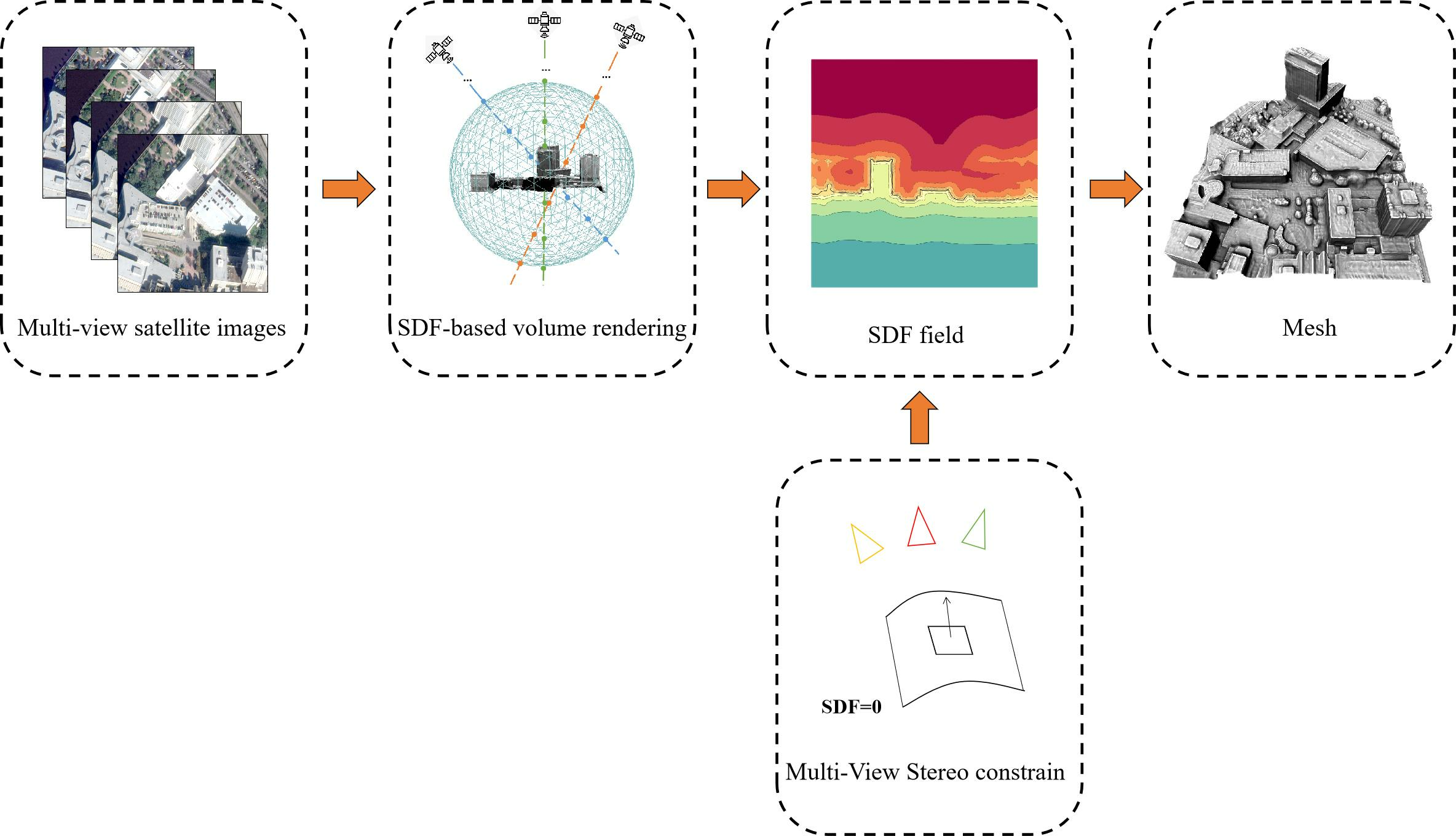
• For the first time, we applied implicit surface reconstruction techniques to satellite imagery, directly generating high-quality 3D mesh models.
• We introduce a robust MVS constraint for accurately learning the implicit surface. By minimizing the photo-consistency between multi-view satellite images, we guarantee that the learned surface is geometry-consistent.
• We introduce the latent appearance in the network architecture to learn the seasonal variations of the satellite images. The learned latent allows for the realistic rendering of novel views with different seasonal appearances, achieving varied seasonal texture mapping for the reconstructed mesh.

2. Related Work

2.1. Pair-Based Satellite Reconstruction

Pair-based satellite reconstruction commonly involves pair selection, stereo rectification, dense stereo matching, triangulation, and depth fusion. Disparity estimation is crucial, and SGM is a popular choice for satellite imagery due to its balanced trade-off between accuracy and computational efficiency [24]. SGM variants, including MGM [5,25], tSGM [26], and Semi-Global Block Matching [27], have been employed to improve efficiency and accuracy in disparity estimation. Furthermore, the deep learning method is progressively being applied to the disparity map estimation of satellite images [28,29,30]. Gómez et al. [28] incorporate the GANet [31] method into the S2P framework to produce disparity maps for satellite images. By overcoming negative disparity and GPU memory limitations, GANet provides enhanced and accurate depth estimations. He et al. [29] introduce a novel dual-scale network for disparity map estimation on high-resolution satellite images. By capturing the dual-scale structures, the network enhances the quality and accuracy of disparity estimation. Marí et al. [30] conducted fine-tuning of established stereo networks, such as Pyramid Stereo Matching [32] and Hierarchical Stereo Matching [33], utilizing a stereo-matching benchmark designed for aerial imagery. This fine-tuning process enhance the networks’ generalization capabilities, improving performance on satellite images.

However, it is essential to acknowledge that these methods primarily focus on pair-wise matching and do not fully exploit the potential of multi-view data. Therefore, due to the lack of redundant view information, these methods struggle to address the challenges posed by seasonal and dynamic variations.

2.2. NeRF-Based Satellite Photogrammetry

Neural Radiance Fields (NeRF) encode 3D scenes by mapping spatial locations to color and volume density through an MLP, generating novel views and high-quality 3D geometry. NeRF excels at handling complex light propagation and reflection compared to traditional matching methods, resulting in more realistic images.

In satellite imagery, the NeRF method has been successfully applied in several studies. S-NeRF leverages the direction of solar rays in the input images to render precise building shadows. Taking it a step further, Sat-NeRF enhances the capabilities of S-NeRF by directly incorporating the actual RPC camera models associated with the satellite images. Additionally, Sat-NeRF introduces a dedicated module to handle transient objects. EO-NeRF [34] leverages the NeRF technique to model the shadows within the scene, ensuring that building shadows align with the scene’s geometry. By utilizing shadow information for geometric inference, it achieves highly accurate and detailed DSM reconstruction. However, it should be noted that these approaches still rely on 2.5D DSMs for representing the 3D geometry.

2.3. Nueal Surface Reconstruction

The potential of volume rendering in reconstructing 3D surfaces has been explored. The NeuS method establishes a functional relationship between the spatial distribution of volume density and the SDF field, ensuring an unbiased volume density distribution on the object surface. By leveraging volume rendering techniques, the SDF field is optimized to enhance the accuracy of surface reconstruction. Additionally, Neuralrecon-W introduces a hybrid voxel- and surface-guided sampling technique that improves ray sampling efficiency around surfaces, resulting in significant advancements in large-scale reconstruction. Geo-NeuS enables the multi-view geometry constraints to optimize the true surface of the SDF field. Motivated by recent advances in monocular geometry prediction, MonoSDF [35] constrains the scene’s SDF using depth and normal cues predicted by general-purpose monocular networks, significantly improving reconstruction quality and optimization time. Neuralangelo [36] combines multiresolution 3D hash grids and neural surface rendering to achieve large-scale dense 3D surface reconstruction from multi-view images. To enhance the efficiency of the NeuS method, NeuS2 [37] utilizes multiresolution hash encodings, optimized second-order derivatives, and a progressive learning strategy, achieving nearly a hundred-fold speedup while maintaining reconstruction quality. While neural surface reconstruction methods have achieved remarkable 3D reconstruction results in ground imagery, successful application in satellite imagery is yet to be realized.

2.4. Photometric 3D Reconstruction

Photometric 3D reconstruction [38,39] aims to recover the three-dimensional structure of a scene from its 2D images by analyzing the changes in lighting conditions across different viewpoints. This method capitalizes on the variations in illumination, shadows, and reflections to infer depth information and create a detailed 3D representation [40]. Rothermel et al. [7] introduce a photometric refinement method to enhance the initial coarse mesh of a 2.5D DSM. This method iteratively optimizes vertex positions to enhance photo-consistency between images, achieving multi-view satellite reconstruction. Similarly, Lv et al. [41] refine the geometric features of a generated 3D mesh model by utilizing the variational energy function [42] among images. Additionally, the subdivision of the 3D mesh is guided by a combination of texture and projection information, resulting in fine-detail reconstruction. These methods rely on coarse initial geometry, while our method reconstructs the mesh directly from satellite images.

2.5. Perspective Approximate for RPC Camera

VisSat proposed a method to approximate the RPC camera model with a pinhole camera model, enabling the application of widely used vision-based techniques to satellite imagery. This advancement allows for the rapid integration of structure from motion (SfM) [43,44,45], multi-view stereo (MVS) [46,47,48], and NeRF into satellite image analysis. Building upon this approximation, S-NeRF successfully applied the pinhole camera-based NeRF method to satellite imagery, facilitating shadow detection, albedo synthesis, and transient object filtering. While the pinhole camera approximation introduces some accuracy loss compared to the RPC camera [28], existing techniques based on perspective projection, such as ray tracing and plane-induced homography, can be directly applied to satellite imagery.

3. Method

We aim to estimate a scene’s SDF based on multi-view satellite images and reconstruct the mesh surface with the zero-level set. The SDF of the scene is learned by the SDF-based volume rendering framework (described in Section 3.1), and the refinement of the surface is achieved through additional constraints imposed by the multi-view images to enhance details (described in Section 3.2). Finally, we introduce our network architecture (described in Section 3.3), loss function, and implementation details (described in Section 3.4). The overview of our method can be seen in Figure 1.

3.1. SDF-Based Volume Rendering

In the volume rendering framework, the color of individual rays is traced across the scene and projected onto the known pixels. Specifically, each ray is traced across the scene and inserted in a normalized sphere at $O_{near}$ and $O_{far}$. Between points $O_{near}$ and $O_{far}$, we sample a set of points denoted as:

$$\{X_i=O_{near}+t_{i}V| i=\mathrm{0,1},\dots ,n-1\}.$$

(1)

The view direction is represented by $V$, $n$ is the number of sample points in each ray, and $t_i$ is a constant value. The rendered color of a ray, $c\left(r\right)$, is obtained through a weighted integration of the predicted colors, $c_i$, at various points along the ray. The color $c\left(r\right)$ of a ray is computed as:

$$c\left(r\right)=\sum _{i=1}^n{T}_i{\alpha }_i{c}_i.$$

(2)

The weight assigned to the predicted color at each point, $X_i$, along the ray, is determined by two factors: the transmittance factor, $T_i$, which represents the probability of the ray reaching that point without encountering any obstructions, and the alpha compositing value, ${\alpha }_i$, which encodes the opacity. These values, $T_i$ and ${\alpha }_i$, are calculated based on the predicted volume density, ${\sigma }_i$, at $X_i$:

$${\alpha }_i=1-exp\left(-{\sigma }_i{\delta }_i\right); T_i=\prod _{j=1}^{i-1}\left(1-{\alpha }_j\right)$$

(3)

where ${\delta }_i$ represents the distance between two consecutive points along the ray, specifically ${\delta }_i=t_{i+1}-t_i$. To train the SDF network with a volume rendering method, a probability density function known as S-density is introduced, denoted as ${\Phi }_s\left(d\right(X_i\left)\right)$, where $d\left(X_i\right)$ represents the signed distance of $X_i$. The opaque density ${\rho }_i$ follows the original definition in NeuS and is calculated as:

$${\rho }_i=max(\frac{\frac{\partial {\Phi }_s\left(d\left(X_i\right)\right)}{\partial t_i}}{{\Phi }_s\left(d\left(X_i\right)\right)},0)$$

(4)

where ${\Phi }_s$ represents the sigmoid function ${\Phi }_s\left(d\right(X_i\left)\right)=\frac{1}{1+exp(-s·d(X_i\left)\right)}$. The trainable parameter $s$ controls the concentration of the opaque density on the object’s surface [19]. When ${\rho }_i$ is decided by SDF value $d\left(X_i\right)$, the transmittance $T_i$ and predicted color adapt to:

$$T_i=\prod _{j=1}^{i-1}(1-{\rho }_j)$$

(5)

$$c\left(r\right)=\sum _{i=1}^n{T}_i{\rho }_i{c}_i$$

(6)

Finally, the SDF and color of the scene are learned by minimizing the loss between the rendered color and the real color of the input images:

$$L_{color}=\sum _{j=1}^m{‖c\left(r_j\right)-c_{GT}\left(r_j\right)‖}_2^2$$

(7)

$m$ is the number of rays in each batch, $c\left(r_j\right)$ is the color predicted by the volume rendering, and the $c_{GT}\left(r_j\right)$ is the pixel color intersected by the ray $r_j$.

3.2. Multi-View Stereo Constrain

Due to variations in solar radiation and atmospheric conditions, satellite images captured at different times may exhibit differences in radiance. However, the underlying texture of the objects remains consistent. Therefore, we use the photo-consistency constraint in MVS to supervise the SDF network, ensuring the learned surface maintains geometric consistency.

The scene is represented by the implicit SDF field, and the extracted surface is the zero-level set of the implicit function:

$$\partial \Omega =\left\{X|d\left(X\right)=0\right\}$$

(8)

We aim to optimize $\partial \Omega$ by MVS constraints across different views. Volume rendering learns the SDF and color in the scene through image rays. Similarly, we search for surface points where the SDF equals zero along these rays. We sample n points along a ray, with corresponding 3D coordinates X. The SDF value at each point is denoted as $d\left(X\right)$. To simplify, we express $d\left(X\right)$ as a function of $t$, i.e., $d\left(t\right)$ (see Formula (1)). The rays that pass through the surface of the object will always have two adjacent sample points, one located inside the object with an SDF value < 0 and the other located outside the object with an SDF value > 0:

$$T=\left\{t_i|d\left(t_i\right)·d\left(t_{i+1}\right)<0\right\}$$

(9)

T is the set of points that satisfy the condition. Based on those sampled points, we can obtain surface points through linear interpolation.

$$t^{*}=\frac{d\left(t_i\right)t_{i+1}-d\left(t_{i+1}\right)t_i}{t_i-t_{i+1}},t_i\in T$$

(10)

$$X^{*}=O_{near}+t^{*}V$$

(11)

For a given ray, there may be multiple $X^{*}$ points. We choose the one with the smallest t, corresponding to the outermost surface point that is least likely to be occluded, for optimization. The normal vector $N$ of a surface point $X^{*}$ can be computed as $N^{*}=\mathsf{\nabla }d\left(X^{*}\right)$. Thus, the plane at the surface point $X^{*}$ is represented as:

$${N^{*T}X}^{*}+l=0$$

(12)

Similar to traditional MVS methods [44,50], we assume that the object’s surface locally approximates a plane. Then, the relationship between the image point $x$ in the pixel patch $p_r$ of the reference image $I_r$ and the corresponding point $x^{\prime }$ in the pixel patch $p_s$ of the source image $I_s$ is described by the plane-induced homography H [23].

$$H=K_r\left(R_{sr}-\frac{N^T{t}_{sr}}{l}\right){K_s}^{-1}$$

(13)

$$x=H{x}^{\prime }$$

(14)

$(N,l)$ represents the plane parameters in the coordinate system of the image $I_s$. $K_s$ and $K_r$ are the intrinsic matrix of $I_s$ and $I_r$, respectively. $R_{sr}$ and $t_{sr}$ denote the relative pose of the image $I_r$ with respect to $I_s$. It is worth noting that the $K$, $R$, and $t$ of the satellite images are approximated by the VisSat method. We convert the color images to grayscale and utilize the normalized cross-correlation (NCC) operator to measure the similarity between different image patches. Considering that the ray emitted from pixel $x$ intersects the object surface at $X^{*}$, we extract a 5 × 5 image patch $p_s$ centered at $x$. By employing Equation (14), we map the pixel positions in the $p_s$ to the $p_r$. The NCC measures the similarity between the image patch $p_s$ and the corresponding patch $p_r$ in the reference image.

$$NCC=\frac{Cov\left(I_s\right(p_s),I_r(p_r\left)\right)}{\sqrt{Var\left(I_s\right(p_s),I_r(p_r\left)\right)}}$$

(15)

$Cov$ and $Var$ represent the covariance and variance functions, respectively. To address transient objects in satellite images and enhance the robustness of the algorithm, we calculate the NCC of the nine reference images and select the top three with the highest scores as the photo-consistency loss:

$$L_{photo}=\frac{\sum _j^m\sum _{i=1}^{3}1-{NCC}_{r_j}\left(I_s\left(p_s\right),I_r\left(p_{ri}\right)\right)}{3m}$$

(16)

Finally, by minimizing the photo-consistency loss $L_{photo}$, the positions and normal vectors of surface points are optimized to their accurate locations and orientations. Figure 2 illustrates ten examples of image patches induced by surface points. The vehicles always dynamically change in satellite imagery. The selection strategy based on the NCC score can effectively filter out image patches containing dynamic vehicles, reducing errors caused by these transient objects.

3.3. Network Architecture

Our methodology samples scene points along the rays emitted from image pixels. Each sampling point encompasses two key parameters: the position $X$ and the viewing direction $V$. As a result, our approach takes the three-dimensional coordinates $X$ and $V$ as input and employs the MLP to predict a one-dimensional SDF, denoted as $d\left(X\right)$, and a three-dimensional color $C$. As illustrated in Figure 3, our network architecture comprises two components: the SDF prediction module ${MLP}_{sdf}$ and the color prediction module ${MLP}_{color}$. Each module is structured with an input layer, multiple hidden layers, and an output layer, utilizing standard fully connected layers and Softplus activation functions. Specifically, the SDF prediction module ${MLP}_{sdf}$ comprises eight hidden layers. The input layer accepts the three-dimensional position vector $X$, while the output layer generates a 256-dimensional feature vector and a one-dimensional SDF $d\left(X\right)$. Furthermore, the skip connections [51] establish a linkage between the input and the output of the fourth layer, thereby facilitating enhanced information flow. The color prediction module ${MLP}_{color}$ consists of four hidden layers, and the output layer produces the color of the sampling point. The input layer comprises five vectors: a three-dimensional sampling point viewing direction, a three-dimensional sampling point position, a three-dimensional normal vector, a 256-dimensional feature vector, and a 256-dimensional latent vector. Notably, the normal vector calculated by the SDF is denoted as $N=\mathsf{\nabla } d\left(X\right)$, and the output feature vector from the SDF prediction module serves directly as the input feature vector for the color prediction module. Similar to [11,14,17], the image-dependent latent vectors $L_j$ (where j represents the image index) are embedded within the input layer to capture radiometric variations between different satellite images.

Furthermore, to improve the representation capabilities of low-dimensional vectors, we apply position encoding to vectors $X$ and $V$ before they enter the network. Specifically, position $X$ is encoded using six distinct frequency components, expanding its dimensionality from 3 to 39. Similarly, the sampling point viewing angle $V$ encoded four different frequency components, augmenting its dimensionality from 3 to 27. Finally, we employ weight normalization [52] to ensure training stability, mitigate potential numerical instability, and foster a robust and reliable learning process.

3.4. Loss Function and Implement Details

Our loss function is:

$$L=L_{color}+\alpha L_{photo}+\beta L_{Eikonal}$$

(17)

The color difference between the ground truth color and the rendered color is denoted as $L_{color}$ (described in Section 3.1). The $L_{photo}$ represents the photo-consistency loss (described in Section 3.2). Additionally,

$$L_{Eikonal}=\frac{1}{nm}\sum _{j=1}^m\sum _{i=1}^n{(\left|\mathsf{\nabla }{d}_{r_j}\left(X_i\right)\right|-1)}^2$$

(18)

$L_{Eikonal}$ is an Eikonal term [53] on the sampled points to regularize SDF values in 3D space.

We approximate the RPC camera model with a pinhole camera described in VisSat and perform bundle adjustment using COLMAP [43]. The normalized sphere of the scene is determined by the sparse points generated from SfM with statistical outlier filtering [54]. The batch size is set to 512 rays for each iteration. The model is trained using the Adam optimizer [55] with parameters (${\beta }_1=0.9$, ${\beta }_2=0.999$), and the total number of iterations is set to 300 k. The initial learning rate is 0.005 and decreases by a factor of ten every 150 k iterations. Training is accelerated using an RTX 3090 GPU, and it takes approximately 8 h to complete the training for one scenario. All experiments are conducted on Ubuntu 20.04 OS within a PyTorch [56] environment. The loss function weight $\alpha$ and $\beta$ are set to 0.5 and 0.1, respectively, for all experiments.

4. Results

4.1. Baseline and Datasets

We evaluate our method on different areas of interest (AOI) of the 2019 IEEE GRSS Data Fusion Contest [57,58]. This dataset includes WorldView-3 (WV3) satellite images with a 0.3 m Ground Sampling Distance (GSD) covering Jacksonville (JAX), Florida, USA, and Omaha (OMA), Nebraska, USA. Additionally, the dataset contains 0.5 m GSD lidar DSMs. The JAX test site consists of 26 images collected between 2014 and 2016. The OMA test site includes 43 images collected between 2014 and 2015 over Omaha (OMA). We compare our method with four baseline methods: (1) S2P pipeline. It utilizes the MGM method and involves pair-wise fusion of 10 manually selected image pairs through median filtering. (2) VisSat. It leverages the PatchMatch [44] method with an approximated pinhole camera. (3) S-NeRF. It is based on NeRF and models the direct and indirect illumination induced by the sun and sky. (4) Sat-NeRF. It is developed from S-NeRF and considers shadows and transient objects. For qualitative analysis, we convert the results of the baseline methods into meshes: the DSMs generated by S-NeRF, S2P, and Sat-NeRF are converted into meshes using GDAL. The 3D point cloud produced by the VisSat method is reconstructed to mesh using the visibility-based Delaunay method [59]. For quantitative analysis, we interpolate our meshes to obtain DSMs for altitude evaluation. The evaluation metrics include mean absolute error (MAE) and median absolute error (MED) compared to the lidar data. Additionally, we introduce an additional metric used by Bosch et al. [60], i.e., the percentage of error below 1 m (Perc-1m). The calculation formulas of the metrics are as follows:

$$MAE=\frac{1}{n}{\sum }_{i=1}^n\left|h_{recon,i}-h_{lidar,i}\right|$$

(19)

$$MED=median\left(\left|h_{recon,i}-h_{lidar,i}\right|\right) for i=\mathrm{1,2},\dots ,n$$

(20)

$$Perc-1m=\frac{\sum _{i\in n}\left[\left|h_{recon,i}-h_{lidar,i}\right|<1\right]}{n}\ast 100\%$$

(21)

where [∙] is the Iverson bracket. $h_{recon,i}$ and $h_{lidar,i}$ represent the elevation value of each pixel of the reconstruction DSM and lidar DSM, respectively. $n$ represents the total number of DSM pixels. To ensure a fair comparison, we evaluate our method on the same AOI as Sat-NeRF and S-NeRF. Furthermore, we select the OMA region with significant appearance differences for latent appearance experiments. Details of the AOIs used in this paper are provided in

Table 1. The details of experiment AOIs. JAX represents Jacksonville. OMA represents Omaha.

AOI	Images	Latitude	Longitude	Covering Size (m)
JAX_004	9	30.358	−81.706	[256 × 265]
JAX_068	17	30.349	−81.664	[256 × 265]
JAX_175	26	30.324	−81.637	[400 × 400]
JAX_214	21	30.316	−81.663	[256 × 265]
JAX_260	15	30.312	−81.663	[256 × 265]
OMA_132	43	41.295	−95.920	[400 × 400]
OMA_212	43	41.295	−95.920	[400 × 400]
OMA_246	43	41.276	−95.921	[400 × 400]
OMA_247	43	41.259	−95.938	[700 × 700]
OMA_248	43	41.267	−95.931	[400 × 400]
OMA_374	43	41.236	−95.920	[400 × 400]

and the images used in each AOI are shown in Figure 4.

4.2. Qualitative Analysis

An overview of the meshes reconstructed by our method is shown in Figure 5. As the figure illustrates, the mesh models reconstructed by our approach exhibit smoothness, detail, low noise, and sharpen-boundary. Buildings are essential targets in satellite reconstruction tasks. Compared to 2.5D DSM models, the 3D mesh can fully represent the building facades. Additionally, the building boundaries reconstructed by our method are distinct, as highlighted in the details presented in Figure 5a,e,f,i. This distinctiveness arises from the fact that building boundaries typically exhibit noticeable color variations, which the volume rendering technique can learn from color disparities to delineate sharp edges. The trees are challenged to be reconstructed due to their varying appearances across multi-date satellite images, influenced by changing seasons. In our network architecture, we have an image-dependent latent vector that encodes the different appearances of different seasons. This capability enables our method to accurately reconstruct trees, as demonstrated in Figure 5a,c. The thin structures in Figure 5h are challenging to represent by the 2.5D DSM, as each pixel in the DSM can only hold a single elevation value. Our method can effectively recover such thin structures, indicating that our implicit SDF representation can handle intricate topological structures. Furthermore, as a multi-view reconstruction approach, we exhibit better robustness in outlier removal compared to pair-based binocular methods. For instance, in the details of Figure 5b, despite the presence of the cars in the images, our mesh surface remains flat and smooth and devoid of elevations caused by the cars. This is attributed to the robust NCC calculation strategy described in Section 3.1, allowing our method to avoid noise caused by dynamic vehicles effectively. A similar scenario arises in Figure 5g, where the specular highlights appear on object surfaces due to the anisotropic material. Our approach, employing the robust NCC calculation strategy, is unaffected by this specular highlight and maintains the smoothness of the reconstructed mesh surface.

Figure 6 shows the mesh results of the AOI areas obtained with our method and baseline methods. We discuss those results from three aspects:

In general, S2P, S-NeRF, and Sat-NeRF exhibit noticeable noises in their results, which may be attributed to the lack of geometric regularization. Upon observation, it is found that transient objects are positively correlated with the presence of noise: the green dotted box regions in Figure 6 represent a rooftop parking lot where vehicles change. While Sat-NeRF considers the influence of transient objects and achieves lower noise than S-NeRF, the noise levels in NeRF-based methods remain significantly higher than other approaches. In comparison, VisSat and our method exhibit lower noise and smoother surfaces. Our approach employs a robust NCC computation strategy (described in Section 3.2), which effectively eliminates the influence of dynamic objects such as vehicles. As a result, the reconstructed mesh surface exhibits smoothness and low noise.

As demonstrated on JAX_004 and JAX_068 in Figure 6, the results from VisSat and S2P appear blurry and distorted, while S-NeRF, Sat-NeRF, and our method, all based on the volume rendering technique, display straight and prominent building contours. This indicates that the volume rendering technique is adept at learning sharp edges from color variation. Examining the building details in JAX_214 and JAX_260, Sat-NeRF and our method demonstrates the ability to capture fine details that other methods fail to reproduce. In contrast, the details in our meshes are closer to lidar data than Sat-NeRF. This is because our method utilized the MVS constraints to enhance reconstruction details. Furthermore, due to the discrete nature of 2.5D DSM, the transformed DSM exhibits jagged artifacts in areas with significant elevation changes, such as sloping roofs or building boundaries (see lidar data detail on JAX_260). However, the mesh model generated by our method is free from such jagged artifacts.

Vegetation often changes in multi-date satellite images, posing challenges for reconstruction. Only our method provides an appropriate and complete representation of tree vegetation (see the details on JAX_004 in Figure 6). The tree results from VisSat appear excessively blurry, while the mean filtering employed by S2P fuses pair-wise point clouds and leads to the loss of some trees. Vegetation and transient objects exhibit dynamic variations, resulting in significant noise in the tree portions of S-NeRF and Sat-NeRF. The robust NCC computational strategy utilized in our approach is advantageous for tree reconstruction, as it requires only three instances of trees with similar textures to achieve reconstruction.

4.3. Quantitative Analysis

The current satellite multi-view reconstruction dataset only provides DSM as the ground truth. Therefore, we interpolated our mesh models into the DSMs for quantitative validation and assessed the altitude error.

Table 2. The error metric of different methods on JAX AOIs. The upward-pointing arrows indicate that a substantial value signifies high accuracy, while the downward-pointing arrows indicate that a minor value signifies high accuracy.

	JAX_004			JAX_068			JAX_214			JAX_260			Mean
	MAE↓	MED↓	Perc-1 m↑	MAE↓	MED↓	Perc-1 m↑	MAE↓	MED↓	Perc-1m↑	MAE↓	MED↓	Perc-1 m↑	MAE↓	MED↓	Perc-1 m↑
VisSat [21]	1.700	0.794	0.523	1.383	0.766	0.702	2.208	1.118	0.346	1.647	0.948	0.384	1.734	0.906	0.489
S2P [5]	2.675	1.570	0.084	1.686	0.796	0.733	2.674	0.698	0.646	2.166	0.854	0.397	2.300	0.980	0.465
S-NeRF [14]	1.831	1.232	0.359	1.496	0.856	0.560	3.686	2.388	0.204	3.245	2.591	0.150	2.565	1.767	0.319
Sat-NeRF [15]	1.417	0.798	0.519	1.276	0.660	0.644	2.126	1.034	0.471	2.429	1.759	0.223	1.812	1.063	0.464
Ours	1.549	0.554	0.583	1.146	0.570	0.751	2.022	0.982	0.499	1.359	0.674	0.449	1.519	0.695	0.571

illustrates the quantitative results of various methods in four AOI regions. Our method consistently achieves the first- or second-best results across metrics and scenes. Additionally, our method outperforms the others regarding the average MAE, MED, and Perc-1m. Sat-NeRF, as an improved version of S-NeRF, surpasses the latter in all metrics. Notably, the quantitative results of VisSat are inferior to our method but superior to S2P. This is because the VisSat method in this paper converts the MVS point cloud to DSM after Delaunay triangulation, effectively reducing noise in the original point cloud. Figure 7 shows that the lack of effective geometric regularization leads to prominent boundaries and noticeable noise in both S-NeRF and Sat-NeRF. S2P, which generates point clouds through stereo pairs and applies median filtering for fusion, encounters significant discrepancies in vegetation between different pairs, resulting in incomplete reconstructions (as observed in JAX_004 in Figure 7). VisSat exhibits lower noise but blurred boundaries. Despite losing the building side geometries during the conversion from 3D mesh to 2.5D DSM, our method achieves clear boundaries and produces smooth results.

4.4. Ablation Study

The overall loss in this paper consists of three parts: color loss, Eikonal loss, and photo loss. To evaluate the impact of those terms, we tested different combinations, and their effects were explored. Figure 8 shows the results. Eikonal loss can constrain the SDF gradient at any position in space, which has a regularizing effect. As a result, Model-2 has less noise than Model-1. When comparing Model-3 and Model-2, the photo-consistent constraint can optimize the SDF network more accurately and smoothly, leading to significant performance improvements.

4.5. Latent Appearance and Texturing

Similar to NeRF-W [11], we embed a low-dimensional latent vector in each image to learn the intrinsic appearance of different satellite images. Utilizing the learned latent vector, we can modify the lighting and appearance of rendered images without altering the underlying 3D geometry.

To achieve this effect, we conducted experiments in the OMA region, which exhibits a temperate continental climate with distinct seasons. The AOI in the OMA_132 consists of satellite images that showcase significant variations, as depicted in the first row of Figure 9. In our approach, we embed the latent vector in an MLP to learn the unique appearance of each image during the training process. When rendering images, replacing the latent vector of different images will result in corresponding appearances. Figure 9 demonstrates how the colors of land, vegetation, and lakes change across different seasons. By capturing these variations, the latent vector can apply them to all images, resulting in a consistent appearance in the rendered images. Based on these rendered images, the reconstruction mesh model can be textured with a consistent appearance, as shown in Figure 10. It is worth noting that due to the approximated pinhole camera, state-of-the-art methods [61] can be directly employed for texturing the mesh. Our method allows for a flexible appearance selection and achieves consistent texture mapping results compared to the original images. We encourage readers to view our accompanying video on the project website (https://jieeeeeeeeeee.github.io/sat-mesh/, accessed on 30 August 2023) to see this effect when rendering paths of novel views.

5. Discussion

5.1. Our One-Stage Method vs. Two-Stage Methods

Our approach is a one-stage method that directly generates mesh models from multi-view satellite images. Popular methods like NASA Ames stereo pipeline [2], MicMac [3], RSP [4,5], and S2P [5] are pair-based two-stage methods. In the case of pair-based methods, views are organized into pairs; each pair is processed using two-view stereo matching methods to create elevation models or point clouds, and then these pair-wise reconstructions are combined to obtain an outcome [62]. However, two-stage methods possess two notable disadvantages: (1). Underutilization of Multi-view Data: These methods primarily focus on pair-wise matching and fail to fully exploit the potential of multi-view data. (2). Error Propagation in Two-Stage Methods: In the case of two-stage methods, a problem in one step can potentially impact subsequent steps, leading to the propagation and accumulation of errors. Consequently, cumulative errors may arise from point clouds to DSMs during the conversion process. As a one-stage approach, our method concurrently processes multiple-view satellite images, effectively utilizing the redundancy inherent in these views. For instance, in Section 3.2, our approach selects the top three highest normalized cross-correlation (NCC) values from nine images for subsequent optimization. This strategy mitigates the adverse effects introduced by dynamic vehicles. Furthermore, our method can capitalize on the multi-view images to learn seasonal variations, enabling texture mapping with consistent seasonal appearances.

5.2. Computing Power

Table 3. Time consumption of our method and compared methods.

Methods	JAX_004	JAX_068	JAX_214	JAX_260
VisSat [21]	3.5 min	7.5 min	9.4 min	5.9 min
S2P [5]	19.2 min	21.5 min	25.4 min	22.6 min
S-NeRF [14]	~8 h	~8 h	~8 h	~8 h
Sat-NeRF [15]	~10 h	~10 h	~10 h	~10 h
Ours	~8 h	~8 h	~8 h	~8 h

compares the time consumption of our method and the reference methods. Among these, both VisSat and S2P complete reconstruction for each scene within 25 min as traditional multi-view reconstruction approaches. On the other hand, methods like S-NeRF, Sat-NeRF, and our approach employ neural network models, and each scene’s reconstruction time extends beyond 8 h. Despite being a one-stage solution, our method’s efficiency does not match traditional methods like S2P and VisSat. Traditional methods benefit from explicit and interpretable optimization parameters, often involving a lesser parameter count. However, within our methodology, the MLP contains a substantial number of parameters, with around 800,000 parameters to be optimized. Moreover, training the MLP demands significant computational resources to ensure effective training and model optimization. In the future, it is essential for us to refer to techniques that accelerate volume rendering training, such as [13,37], to reduce the computational time of our method.

The memory usage of our method on different datasets is shown in

Table 4. GPU memory consumption of our method. The unit of the GPU memory in the table is MB.

	JAX_004	JAX_068	JAX_214	JAX_260	OMA_132	OMA_212	OMA_246	OMA_247	OMA_374
Input images	9	17	21	15	43	43	43	43	43
Our method without MVS constrain	5027	5047	5049	5047	5267	5267	5267	5267	5267
Our method with MVS constrain	5671	5691	5691	5691	5911	5911	5911	5911	5911

. From the table, it is evident that the GPU memory consumption of our method is positively correlated with the number of input images. Comparing the JAX_004 and OMA_212 datasets, despite an increase of 34 images, the GPU memory only rises by 4%. This is attributed to our method’s primary GPU memory consumption being influenced by scene sampling points, which remain consistent regardless of the image number. During training, our method processes 512 rays, each of which samples 128 scene points. These 65,536 points encompass variables like transmittance ($T$), opaque density ($\rho$), color ($C$), and others, which consume around 4.5 GB of GPU memory.

The MVS constraint requires additional memory storage for variables such as NCC and homography matrix ($H$) at the sampling points. As a result, the GPU memory increases by approximately 12% when photo-consistency operations are included (refer to the second and third columns of Table 4). In summary, the input image count for multi-view satellite reconstruction tasks typically remains within 50 images. Our method’s GPU memory consumption for each AOI remains within 6 GB.

6. Conclusions

We propose Sat-Mesh, a novel method for satellite implicit surface reconstruction. Our approach leverages multi-view satellite imagery to learn the scene’s SDF and employs the marching cubes algorithm to generate a mesh model. In contrast to popular pair-based satellite reconstruction methods, our approach fully utilizes the redundancy of multi-view information and employs a more robust photo-consistency constraint to improve the accuracy of the implicit surface. Additionally, we learn the appearance attributes of images during the training process, allowing us to render appearance-consistent images by learned latent vectors. By mapping rendered images with different appearances, we obtain texture meshes with diverse seasonal features. However, our method has some limitations. Firstly, it does not consider the influence of shadows on the reconstruction. Secondly, it has relatively low computational efficiency. Lastly, we believe that re-implementing our method with a high-precision RPC model would be beneficial. We hope that future research can address these challenges and improve this work.

References

1. Zhao, Q.; Yu, L.; Du, Z.; Peng, D.; Hao, P.; Zhang, Y.; Gong, P. An overview of the applications of earth observation satellite data: Impacts and future trends. Remote Sens. 2022, 14, 1863. [Google Scholar] [CrossRef]
2. Beyer, R.A.; Alexandrov, O.; McMichael, S. The Ames Stereo Pipeline: NASA’s open source software for deriving and processing terrain data. Earth Space Sci. 2018, 5, 537–548. [Google Scholar] [CrossRef]
3. Rupnik, E.; Daakir, M.; Pierrot Deseilligny, M. MicMac—A free, open-source solution for photogrammetry. Open Geospat. Data Softw. Stand. 2017, 2, 14. [Google Scholar] [CrossRef]
4. Qin, R. Rpc stereo processor (rsp)—A software package for digital surface model and orthophoto generation from satellite stereo imagery. ISPRS Ann. Photogramm. Remote Sens. Spat. Inf. Sci. 2016, 3, 77–82. [Google Scholar] [CrossRef]
5. Facciolo, G.; De Franchis, C.; Meinhardt-Llopis, E. Automatic 3D reconstruction from multi-date satellite images. In Proceedings of the IEEE Conference on Computer Vision and Pattern Recognition Workshops, Honolulu, HI, USA, 21–26 July 2017; pp. 57–66. [Google Scholar]
6. Hirschmuller, H. Stereo processing by semiglobal matching and mutual information. IEEE Trans. Pattern Anal. Mach. Intell. 2007, 30, 328–341. [Google Scholar] [CrossRef] [PubMed]
7. Rothermel, M.; Gong, K.; Fritsch, D.; Schindler, K.; Haala, N. Photometric multi-view mesh refinement for high-resolution satellite images. ISPRS J. Photogramm. Remote Sens. 2020, 166, 52–62. [Google Scholar] [CrossRef]
8. Bullinger, S.; Bodensteiner, C.; Arens, M. 3D Surface Reconstruction From Multi-Date Satellite Images. arXiv 2021, arXiv:2102.02502. [Google Scholar] [CrossRef]
9. Park, S.-Y.; Seo, D.; Lee, M.-J. GEMVS: A novel approach for automatic 3D reconstruction from uncalibrated multi-view Google Earth images using multi-view stereo and projective to metric 3D homography transformation. Int. J. Remote Sens. 2023, 44, 3005–3030. [Google Scholar] [CrossRef]
10. Mildenhall, B.; Srinivasan, P.P.; Tancik, M.; Barron, J.T.; Ramamoorthi, R.; Ng, R. Nerf: Representing scenes as neural radiance fields for view synthesis. Commun. ACM 2021, 65, 99–106. [Google Scholar] [CrossRef]
11. Martin-Brualla, R.; Radwan, N.; Sajjadi, M.S.; Barron, J.T.; Dosovitskiy, A.; Duckworth, D. Nerf in the wild: Neural radiance fields for unconstrained photo collections. In Proceedings of the IEEE/CVF Conference on Computer Vision and Pattern Recognition, Nashville, TN, USA, 20–25 June 2021. [Google Scholar]
12. Barron, J.T.; Mildenhall, B.; Verbin, D.; Srinivasan, P.P.; Hedman, P. Mip-nerf 360: Unbounded anti-aliased neural radiance fields. In Proceedings of the IEEE/CVF Conference on Computer Vision and Pattern Recognition, New Orleans, LA, USA, 18–24 June 2022; pp. 5470–5479. [Google Scholar]
13. Müller, T.; Evans, A.; Schied, C.; Keller, A. Instant neural graphics primitives with a multiresolution hash encoding. ACM Trans. Graph. 2022, 41, 1–15. [Google Scholar] [CrossRef]
14. Derksen, D.; Izzo, D. Shadow neural radiance fields for multi-view satellite photogrammetry. In Proceedings of the IEEE/CVF Conference on Computer Vision and Pattern Recognition, Nashville, TN, USA, 19–25 June 2021; pp. 1152–1161. [Google Scholar]
15. Marí, R.; Facciolo, G.; Ehret, T. Sat-nerf: Learning multi-view satellite photogrammetry with transient objects and shadow modeling using rpc cameras. In Proceedings of the IEEE/CVF Conference on Computer Vision and Pattern Recognition, New Orleans, LA, USA, 19–20 June 2022; pp. 1311–1321. [Google Scholar]
16. Fu, Q.; Xu, Q.; Ong, Y.S.; Tao, W. Geo-neus: Geometry-consistent neural implicit surfaces learning for multi-view reconstruction. Adv. Neural Inf. Process. Syst. 2022, 35, 3403–3416. [Google Scholar]
17. Sun, J.; Chen, X.; Wang, Q.; Li, Z.; Averbuch-Elor, H.; Zhou, X.; Snavely, N. Neural 3d reconstruction in the wild. In Proceedings of the ACM SIGGRAPH 2022 Conference Proceedings, Vancouver, BC, Canada, 7–11 August 2022; pp. 1–9. [Google Scholar]
18. Wang, Y.; Skorokhodov, I.; Wonka, P. PET-NeuS: Positional Encoding Tri-Planes for Neural Surfaces. In Proceedings of the IEEE/CVF Conference on Computer Vision and Pattern Recognition, Vancouver, BC, Canada, 17–24 June 2023; pp. 12598–12607. [Google Scholar]
19. Wang, P.; Liu, L.; Liu, Y.; Theobalt, C.; Komura, T.; Wang, W. Neus: Learning neural implicit surfaces by volume rendering for multi-view reconstruction. arXiv 2021, arXiv:2106.10689. [Google Scholar]
20. Bojanowski, P.; Joulin, A.; Lopez-Paz, D.; Szlam, A. Optimizing the latent space of generative networks. arXiv 2017, arXiv:1707.05776. [Google Scholar]
21. Zhang, K.; Snavely, N.; Sun, J. Leveraging vision reconstruction pipelines for satellite imagery. In Proceedings of the IEEE/CVF International Conference on Computer Vision Workshops, Seoul, Republic of Korea, 27–28 October 2019. [Google Scholar]
22. Kajiya, J.T.; Von Herzen, B.P. Ray tracing volume densities. ACM SIGGRAPH Comput. Graph. 1984, 18, 165–174. [Google Scholar] [CrossRef]
23. Hartley, R.; Zisserman, A. Multiple View Geometry in Computer Vision; Cambridge University Press: Cambridge, UK, 2003. [Google Scholar]
24. Zabih, R.; Woodfill, J. Non-parametric local transforms for computing visual correspondence. In Proceedings of the Computer Vision—ECCV’94: Third European Conference on Computer Vision, Stockholm, Sweden, 2–6 May 1994; Springer: Berlin/Heidelberg, Germany; Volume II 3, pp. 151–158. [Google Scholar]
25. Facciolo, G.; De Franchis, C.; Meinhardt, E. MGM: A significantly more global matching for stereovision. In Proceedings of the BMVC 2015, Swansea, UK, 7–10 September 2015. [Google Scholar]
26. Rothermel, M.; Wenzel, K.; Fritsch, D.; Haala, N. SURE: Photogrammetric surface reconstruction from imagery. In Proceedings of the LC3D Workshop, Berlin, Germany, 4–5 December 2012; Volume 8. [Google Scholar]
27. Lastilla, L.; Ravanelli, R.; Fratarcangeli, F.; Di Rita, M.; Nascetti, A.; Crespi, M. FOSS4G DATE for DSM generation: Sensitivity analysis of the semi-global block matching parameters. Int. Arch. Photogramm. Remote Sens. Spat. Inf. Sci. 2019, 42, 67–72. [Google Scholar] [CrossRef]
28. Gómez, A.; Randall, G.; Facciolo, G.; von Gioi, R.G. An experimental comparison of multi-view stereo approaches on satellite images. In Proceedings of the IEEE/CVF Winter Conference on Applications of Computer Vision, Waikoloa, HI, USA, 3–8 January 2022; pp. 844–853. [Google Scholar]
29. He, S.; Zhou, R.; Li, S.; Jiang, S.; Jiang, W. Disparity estimation of high-resolution remote sensing images with dual-scale matching network. Remote Sens. 2021, 13, 5050. [Google Scholar] [CrossRef]
30. Marí, R.; Ehret, T.; Facciolo, G. Disparity Estimation Networks for Aerial and High-Resolution Satellite Images: A Review. Image Process. Line 2022, 12, 501–526. [Google Scholar] [CrossRef]
31. Zhang, F.; Prisacariu, V.; Yang, R.; Torr, P.H. Ga-net: Guided aggregation net for end-to-end stereo matching. In Proceedings of the IEEE/CVF Conference on Computer Vision and Pattern Recognition, Long Beach, CA, USA, 15–20 June 2019; pp. 185–194. [Google Scholar]
32. Chang, J.-R.; Chen, Y.-S. Pyramid stereo matching network. In Proceedings of the IEEE conference on Computer Vision and Pattern Recognition, Salt Lake City, UT, USA, 18–23 June 2018; pp. 5410–5418. [Google Scholar]
33. Yang, G.; Manela, J.; Happold, M.; Ramanan, D. Hierarchical deep stereo matching on high-resolution images. In Proceedings of the IEEE/CVF Conference on Computer Vision and Pattern Recognition, Long Beach, CA, USA, 15–20 June 2019; pp. 5515–5524. [Google Scholar]
34. Marí, R.; Facciolo, G.; Ehret, T. Multi-Date Earth Observation NeRF: The Detail Is in the Shadows. In Proceedings of the IEEE/CVF Conference on Computer Vision and Pattern Recognition, Vancouver, BC, Canada, 17–24 June 2023; pp. 2034–2044. [Google Scholar]
35. Yu, Z.; Peng, S.; Niemeyer, M.; Sattler, T.; Geiger, A. Monosdf: Exploring monocular geometric cues for neural implicit surface reconstruction. Adv. Neural Inf. Process. Syst. 2022, 35, 25018–25032. [Google Scholar]
36. Li, Z.; Müller, T.; Evans, A.; Taylor, R.H.; Unberath, M.; Liu, M.-Y.; Lin, C.-H. Neuralangelo: High-Fidelity Neural Surface Reconstruction. In Proceedings of the IEEE/CVF Conference on Computer Vision and Pattern Recognition, Vancouver, BC, Canada, 17–24 June 2023; pp. 8456–8465. [Google Scholar]
37. Wang, Y.; Han, Q.; Habermann, M.; Daniilidis, K.; Theobalt, C.; Liu, L. Neus2: Fast learning of neural implicit surfaces for multi-view reconstruction. arXiv 2022, arXiv:2212.05231. [Google Scholar]
38. Ju, Y.; Peng, Y.; Jian, M.; Gao, F.; Dong, J. Learning conditional photometric stereo with high-resolution features. Comput. Vis. Media 2022, 8, 105–118. [Google Scholar] [CrossRef]
39. Chen, G.; Han, K.; Wong, K.-Y.K. PS-FCN: A flexible learning framework for photometric stereo. In Proceedings of the European conference on computer vision (ECCV), Munich, Germany, 8–14 September 2018; pp. 3–18. [Google Scholar]
40. Yao, Z.; Li, K.; Fu, Y.; Hu, H.; Shi, B. Gps-net: Graph-based photometric stereo network. Adv. Neural Inf. Process. Syst. 2020, 33, 10306–10316. [Google Scholar]
41. Lv, B.; Liu, J.; Wang, P.; Yasir, M. DSM Generation from Multi-View High-Resolution Satellite Images Based on the Photometric Mesh Refinement Method. Remote Sens. 2022, 14, 6259. [Google Scholar] [CrossRef]
42. Qu, Y.; Yan, Q.; Yang, J.; Xiao, T.; Deng, F. Total Differential Photometric Mesh Refinement with Self-Adapted Mesh Denoising. Photonics 2022, 10, 20. [Google Scholar] [CrossRef]
43. Schonberger, J.L.; Frahm, J.-M. Structure-from-motion revisited. In Proceedings of the IEEE Conference on Computer Vision and Pattern Recognition, Las Vegas, NV, USA, 27–30 June 2016; pp. 4104–4113. [Google Scholar]
44. Schönberger, J.L.; Zheng, E.; Frahm, J.-M.; Pollefeys, M. Pixelwise view selection for unstructured multi-view stereo. In Proceedings of the Computer Vision–ECCV 2016: 14th European Conference, Amsterdam, The Netherlands, 11–14 October 2016; Part III 14. pp. 501–518. [Google Scholar]
45. Xiao, T.; Wang, X.; Deng, F.; Heipke, C. Sequential Cycle Consistency Inference for Eliminating Incorrect Relative Orientations in Structure from Motion. PFG–J. Photogramm. Remote Sens. Geoinf. Sci. 2021, 89, 233–249. [Google Scholar] [CrossRef]
46. Furukawa, Y.; Hernández, C. Multi-view stereo: A tutorial. In Foundations and Trends® in Computer Graphics and Vision; Now Publishers Inc.: Hanover, MA, USA, 2015; Volume 9, pp. 1–148. [Google Scholar]
47. Romanoni, A.; Matteucci, M. Tapa-mvs: Textureless-aware patchmatch multi-view stereo. In Proceedings of the IEEE/CVF International Conference on Computer Vision, Seoul, Republic of Korea, 27 October–2 November 2019; pp. 10413–10422. [Google Scholar]
48. Xu, Q.; Tao, W. Multi-Scale Geometric Consistency Guided Multi-View Stereo. In Proceedings of the Computer Vision and Pattern Recognition (CVPR), Long Beach, CA, USA, 15–20 June 2019. [Google Scholar]
49. Lorensen, W.E.; Cline, H.E. Marching cubes: A high resolution 3D surface construction algorithm. In Seminal Graphics: Pioneering Efforts That Shaped the Field; Association for Computing Machinery: New York, NY, USA, 1998; pp. 347–353. [Google Scholar]
50. Furukawa, Y.; Ponce, J. Accurate, dense, and robust multi-view stereopsis (pmvs). In Proceedings of the IEEE Computer Society Conference on Computer Vision and Pattern Recognition, Minneapolis, MN, USA, 18–23 June 2007. [Google Scholar]
51. Park, J.J.; Florence, P.; Straub, J.; Newcombe, R.; Lovegrove, S. Deepsdf: Learning continuous signed distance functions for shape representation. In Proceedings of the IEEE/CVF Conference on Computer Vision and Pattern Recognition, Long Beach, CA, USA, 15–20 June 2019; pp. 165–174. [Google Scholar]
52. Salimans, T.; Kingma, D.P. Weight normalization: A simple reparameterization to accelerate training of deep neural networks. arXiv 2016, arXiv:1602.07868. [Google Scholar]
53. Gropp, A.; Yariv, L.; Haim, N.; Atzmon, M.; Lipman, Y. Implicit geometric regularization for learning shapes. arXiv 2020, arXiv:2002.10099. [Google Scholar]
54. Zhou, Q.-Y.; Park, J.; Koltun, V. Open3D: A modern library for 3D data processing. arXiv 2018, arXiv:1801.09847. [Google Scholar]
55. Kingma, D.P.; Ba, J. Adam: A method for stochastic optimization. arXiv 2014, arXiv:1412.6980. [Google Scholar]
56. Paszke, A.; Gross, S.; Massa, F.; Lerer, A.; Bradbury, J.; Chanan, G.; Killeen, T.; Lin, Z.; Gimelshein, N.; Antiga, L. Pytorch: An imperative style, high-performance deep learning library. arXiv 2019, arXiv:1912.01703. [Google Scholar]
57. Bosch, M.; Foster, K.; Christie, G.; Wang, S.; Hager, G.D.; Brown, M. Semantic stereo for incidental satellite images. In Proceedings of the 2019 IEEE Winter Conference on Applications of Computer Vision (WACV), Waikoloa, HI, USA, 7–11 January 2019; pp. 1524–1532. [Google Scholar]
58. Le Saux, B.; Yokoya, N.; Hänsch, R.; Brown, M. 2019 ieee grss data fusion contest: Large-scale semantic 3d reconstruction. IEEE Geosci. Remote Sens. Mag. (GRSM) 2019, 7, 33–36. [Google Scholar] [CrossRef]
59. Delaunoy, A.; Prados, E. Gradient flows for optimizing triangular mesh-based surfaces: Applications to 3d reconstruction problems dealing with visibility. Int. J. Comput. Vis. 2011, 95, 100–123. [Google Scholar] [CrossRef]
60. Bosch, M.; Kurtz, Z.; Hagstrom, S.; Brown, M. A multiple view stereo benchmark for satellite imagery. In Proceedings of the 2016 IEEE Applied Imagery Pattern Recognition Workshop (AIPR), Washington, DC, USA, 18–20 October 2016; pp. 1–9. [Google Scholar]
61. Waechter, M.; Moehrle, N.; Goesele, M. Let there be color! Large-scale texturing of 3D reconstructions. In Proceedings of the Computer Vision–ECCV 2014: 13th European Conference, Zurich, Switzerland, 6–12 September 2014; Part V 13. pp. 836–850. [Google Scholar]
62. Gómez, A.; Randall, G.; Facciolo, G.; von Gioi, R.G. Improving the Pair Selection and the Model Fusion Steps of Satellite Multi-View Stereo Pipelines. In Proceedings of the IEEE/CVF Winter Conference on Applications of Computer Vision, Seoul, Republic of Korea, 27 October–2 November 2019; pp. 6344–6353. [Google Scholar]
Figure 1. Overview of Sat-Mesh. Each input satellite imagery emits rays and samples the scene points along those rays. The positions and directions of the sampled points are input to two MLPs, which predict the SDF and color, respectively. We can learn the scene’s SDF from the pixel color through the SDF-based volume rendering process. Additionally, we apply the MVS constraint on the surface where SDF = 0. By minimizing photo-consistency loss, we guarantee that the learned surface is geometry-consistent. Finally, the mesh is extracted from the learned SDF using the marching cubes algorithm [49].
Remotesensing 15 04297 g001
Figure 2. Ten examples of image patches induced by surface points. The S represents the image patch of the source image, and Ri denotes the image patch in the i-th reference image. The static image patches indicate that the texture induced by the surface point remains static in the image. In contrast, the dynamic image patches indicate that the texture induced by the surface point varies across different images. While dealing with the dynamic image patches, the blue boxes highlight the three patches with the highest NCC among the nine reference images. This strategy effectively filters out the dynamic vehicles and improves the accuracy and reliability of the NCC calculations.
Remotesensing 15 04297 g002
Figure 3. Our network architecture.
Remotesensing 15 04297 g003
Figure 4. The images used in each AOI.
Remotesensing 15 04297 g004
Figure 5. Overview of the meshes reconstructed by our method. (ai) presents the mesh reconstruction results for various AOIs, along with images and mesh details. The red boxes represent the enlarged regions.
Remotesensing 15 04297 g005
Figure 6. The mesh results on JAX AOIs. Top to bottom: JAX_004, JAX_068, JAX_214, JAX_260. The red boxes show the enlarged mesh details.
Remotesensing 15 04297 g006
Figure 7. The DSMs produced by different methods on JAX AOIs. Top to bottom: JAX_004, JAX_068, JAX_214, JAX_260.
Remotesensing 15 04297 g007
Figure 8. Mesh quality of ablation models. The upward-pointing arrows indicate that a substantial value signifies high accuracy, while the downward-pointing arrows indicate that a minor value signifies high accuracy.
Remotesensing 15 04297 g008
Figure 9. Rendered images with different latent appearances based on three different capture dates: Image_1 captured on 15 August 2015, Image_2 captured on 20 February 2015, and Image_3 captured on 7 January 2015. Those three images are picked from the origin images collection (see red box in the first row).
Remotesensing 15 04297 g009
Figure 10. Textured mesh using rendered images with different latent appearances.
Remotesensing 15 04297 g010