Article

Fast Variational Bayesian Inference for Space-Time Adaptive Processing

National Key Laboratory of Radar Signal Processing, Xidian University, Xi’an 710071, China
*
Author to whom correspondence should be addressed.
Remote Sens. 2023, 15(17), 4334; https://doi.org/10.3390/rs15174334
Submission received: 7 August 2023 / Revised: 28 August 2023 / Accepted: 31 August 2023 / Published: 2 September 2023

Abstract

:
Space-time adaptive processing (STAP) approaches based on sparse Bayesian learning (SBL) have attracted much attention for the benefit of reducing the training samples requirement and accurately recovering sparse signals. However, it has the problem of a heavy computational burden and slow convergence speed. To improve the convergence speed, the variational Bayesian inference (VBI) is introduced to STAP in this paper. Moreover, to improve computing efficiency, a fast iterative algorithm is derived. By constructing a new atoms selection rule, the dimension of the matrix inverse problem can be substantially reduced. Experiments conducted on the simulated data and measured data verify that the proposed algorithm has excellent clutter suppression and target detection performance.

1. Introduction

Space-time adaptive processing (STAP) is widely studied and applied in airborne phased array radar for clutter suppression and target detection [1,2,3,4,5]. The performance of STAP is related to the clutter plus noise covariance matrix (CNCM), which is estimated by the training samples adjacent to the cell under test (CUT). More than two times the system degrees of freedom (DOFs) of independent and identically distributed (IID) training samples are required to estimate the CNCM [6,7]. However, it is difficult to obtain enough training samples in a practical environment.
Various algorithms have been proposed to improve the STAP performance with a small number of training samples. Reduced-rank (RR) approaches make use of the structural characteristics of the covariance matrix to reduce the requirement for samples, such as principal components (PC), the multistage winner filter (MWF), and cross-spectral metric (CSM) [8,9,10,11]. Reduced-dimension (RD) approaches reduce the requirement for samples by selecting space-time or angle-Doppler channels, such as joint-domain localization (JDL), the extend factor approach (EFA), and auxiliary channel processor (ACP) [12,13,14,15]. However, the performance of the RR or RD approaches is affected due to complex practical environments. Knowledge-aided (KA) [16,17,18] approaches use prior knowledge to improve clutter suppression performance. Nevertheless, it is hard to obtain precise prior knowledge. Additionally, some covariance estimation algorithms in limited samples have been proposed, such as the fast maximum likelihood (ML) estimation [19], rank-constrained ML estimation [20], knowledge-aided ML estimation [21], and distribution-free covariance estimation [22]. These approaches are sensitive to model mismatch.
Motivated by the compressed sensing (CS) theory, sparse recovery STAP (SR-STAP) methods have attracted much attention over the last few years [23,24,25,26]. Using the norm minimization method and the sparsity of the clutter spectrum, SR-STAP approaches can improve the clutter suppression performance with few samples or even a single sample. Currently, several SR methods have been proposed. In [27], a convex optimization algorithm named the focal underdetermined system solver (FOCUSS) was proposed, which uses the p norm penalty to relax the cost function. This kind of algorithm requires a suitable regularization parameter. However, the parameter chosen empirically is not robust to environmental change. A greedy pursuit approach, an orthogonal matching pursuit, is presented in [28]. It performs well when the signal sparsity is known. The difficulty in obtaining signal sparsity in practice limits the application of this type of approach. For its self-regularizing nature, sparse Bayesian learning (SBL) has received much attention and has been applied to STAP [29,30,31]. However, the problems of heavy computational burden and slow convergence speed prevent its practical application.
Variational Bayesian inference (VBI) can be seen as a Bayesian approximate method that deals with the SR problem by maximizing a lower bound of likelihood function [32,33,34]. Compared with SBL, VBI replaces the point estimation of parameters with approximate posterior distribution estimates, which gives it a fast convergence speed. The VBI has been widely used in the fields of engineering and signal processing, some of which include model degradation analysis [35], statistical properties estimation [36], and Orthogonal Time Frequency Space (OTFS) modulation [37]. In this paper, the VBI algorithm with multiple measurement vectors (MMV) is introduced in STAP (M-VBI-STAP). Because of the matrix inverse operation, the computational burden is still heavy. To reduce the computational complexity, a fast STAP algorithm based on VBI is proposed. The following are the main contributions of this paper:
(1)
The frame of VBI with multiple measurement vectors is generalized to the STAP application. This allows for an increase in convergence speed.
(2)
In order to improve computational efficiency, a fast STAP algorithm based on VBI (M-FVBI-STAP) is proposed. A new atoms selection rule is constructed, which is able to substantially reduce the dimension of the matrix inverse problem.
(3)
Numerous experiment results on simulated data and measured data illustrate that the proposed algorithm can achieve better clutter suppression and target detection performance.
The remainder of this paper is outlined as follows. The signal model and Bayesian model are introduced in Section 2. In Section 3, the VBI algorithm is extended to STAP and proposes a fast STAP method based on VBI. Computational complexity analysis is detailed in Section 4. Section 5 shows the experimental results. The conclusions are presented in Section 6.
Notation: Matrices, vectors, and scalar quantities are denoted by boldface uppercase, boldface lowercase, and lightface letters, respectively. The symbols and I represent the complex filed and the identity matrix. For a matrix X , ( X ) 1 , ( X ) T , and ( X ) H denote the inverse, transpose and conjugate transpose of X , respectively. 2 , 2 , 0 , and F denote the 2 , 2 , 0 and Frobenius norms, respectively. d i a g ( x ) denotes a diagonal matrix whose diagonal element is x . stands for the kronecker product. denotes the expectation.

2. Signal Model and Bayesian Model

2.1. Signal Model

The system under consideration is a side-looking airborne-phased array radar with a uniform linear array (ULA), which consists of N elements spaced at half a wavelength. The radar transmits M pulses at a constant pulse repetition frequency (PRF) in a coherent processing interval (CPI). Ignoring the range ambiguity, the received space-time signal is modeled as
x = x c + x t + n   = i = 1 N c α i s ( f d , i , f s , i ) + α t a t + n
where x c is the clutter component; N c denotes the number of clutter patches for each range cell; x t stands for the target component; n denotes the complex white Gaussian noise; f d , i and f s , i are the normalized Doppler frequency and normalized spatial frequency; α t and α i are the complex amplitude of the target and the i-th clutter patch, respectively; a t represents the space-time steering vector of the target and s ( f d , i , f s , i ) is the space-time steering vector of the clutter with the form
s ( f d , i , f s , i ) = s t ( f d , i ) s s ( f s , i )
where s t ( f d , i ) and s s ( f s , i ) are the temporal steering vector and spatial steering vector
s t ( f d , i ) = [ 1 , exp ( j 2 π f d , i ) , , exp ( j 2 π ( M 1 ) f d , i ) ] T
s s ( f s , i ) = [ 1 , exp ( j 2 π f s , i ) , , exp ( j 2 π ( N 1 ) f s , i ) ] T
The optimum weight of the STAP filter is obtained from the problem,
{ min w w H R c + n w s . t . w H a t = 1 .
The optimum weight of the STAP filter can be acquired by
w o p t = R c + n 1 a t a t H R c + n 1 a t .
This assumes that the clutter and noise components are mutually uncorrelated. Then, the clutter plus noise covariance matrix (CNCM) can be written as
R c + n = R c + R n   = x x H + σ 2 I
where R c M N × M N and R n M N × M N represent the CCM and noise covariance matrix and σ 2 is the power of the noise.
For the SR-STAP algorithms, the angle-Doppler plane is uniformly discretized into K = N s N d grids. Here, N s = ρ s N and N d = ρ d M are the number of angle bins, and Doppler bins, respectively. The received signal X N M × L from L IID training samples can be written as
X = Φ A + N
where Φ = [ s 1 , s 2 , s K ] M N × K is the dictionary matrix, A = [ α 1 , α 2 , , α L ] K × L denotes the sparse coefficient matrix, and N = [ n 1 , n 2 , , n L ] M N × L represents the noise matrix.
The angle-Doppler profile can be estimated by solving the following problem:
A = arg min A A 2 , 0 s . t . X Φ A F 2 ε
where ε is the noise error tolerance. Thus, the CNCM can be estimated by
R ˜ c + n = 1 L l = 1 L Φ d i a g ( α l 2 ) Φ H + σ 2 I M N .

2.2. Bayesian Model

From a Bayesian perspective, noise is assumed to be a zero-mean complex of Gaussian distribution. Then, the complex Gaussian likelihood for the X can be modeled as
p ( X | A , σ 2 ) = l = 1 L C N ( x l | Φ α l , δ 1 I M N )
where δ = σ 2 is the noise precision. According to the conjugate prior principle [38], the δ follows a Gamma distribution,
p ( δ ) = G a m m a ( δ | c , d )
where G a m m a ( δ | c , d ) = d c γ ( c ) δ c 1 exp ( d δ ) , γ ( c ) is the Gamma function and c and d represent the shape parameter and scale parameter.
To model the sparse coefficient, a complex Gaussian prior is employed first for each column of A
p ( α l | λ ) = k = 1 K C N ( a k , l | 0 , λ k 1 )
where λ = [ λ 1 , , λ k , , λ K ] T . A Gamma prior is assigned on the hyper-parameter λ k
p ( λ k ) = G a m m a ( λ k | a , b )
In a word, the Bayesian model of the received signal has been established. Figure 1 shows the corresponding graphical model. Each node represents a conditional probability density.

3. Proposed Algorithm

In this section, a VBI-based STAP algorithm is derived for the MMV case. Then, a fast iterative structure is proposed to improve the computational efficiency of M-VBI-STAP.

3.1. VBI Algorithm

The set of hiding variables for the Bayesian model denotes Ω = [ A , λ , δ ] . The marginal likelihood function p ( X ) needs to be calculated to obtain the closed form of the posterior distribution p ( Ω | X ) . Since p ( X ) is intractable, it can be decomposed as
ln p ( X ) = L ( q ) + K L ( q | p )
with
L ( q ) = q ( Ω ) ln ( p ( X , Ω ) q ( Ω ) ) d Ω
and
K L ( q | p ) = q ( Ω ) ln ( p ( Ω | X ) q ( Ω ) ) d Ω
where q ( Ω ) denotes a variational distribution, L ( q ) is the lower bound of ln p ( X ) , and K L ( q | p ) represents the Kullback–Leibler divergence between the p ( Ω | X ) and q ( Ω ) regularization parameters. The VBI algorithm approximates the posterior distribution using the factorized variable distribution. Assuming the variables are independent of each other, the factorized variable distribution can be expressed as
q ( Ω ) = q ( X ) q ( λ ) q ( δ ) .
Maximizing L ( q ) , the optimal factorized variable distribution is
ln q ( Ω ) = ln p ( X , Ω ) q ( Ω \ Ω i ) + const
where Ω \ Ω i means removing Ω i from Ω , and
p ( X , Ω ) = p ( X | A , λ , δ ) p ( A | λ ) p ( λ ) p ( δ )
Combining Equations (19) and (20), the following gives the iterative update procedure of the variational parameters:
(1)
update A
ln q ( A ) = ln p ( X | A , λ , δ ) + ln p ( A | λ ) q ( Ω \ X ) + const   = δ l = 1 L x l Φ α l 2 2 + l = 1 L α l H d i a g ( λ ) α l + const
It can be found that q ( A ) obeys the Gaussian distribution
q ( A ) = l = 1 L C N ( α l | μ l , Σ )
where
μ l = δ Σ Φ H x l
Σ = d i a g ( λ ) d i a g ( λ ) Φ H ( δ I M N + Φ d i a g ( λ ) Φ H ) 1 Φ d i a g ( λ )
(2)
Update λ
ln q ( λ ) = ln p ( A | λ ) + ln p ( λ ) q ( Ω \ λ ) + const   = k = 1 K [ ( a + L 1 ) ln λ k ( b + l = 1 L a k , l a k , l H ) λ k ]
From Equation (25), q ( λ ) follows Gamma distribution and λ k can be obtained by
λ k = a + L b + l = 1 L a k , l a k , l H
where a k , l a k , l H = μ k , l 2 + Σ k , k , μ k , l is the k-th element of μ l and Σ k , k denotes the k-th main diagonal element of Σ .
(3)
Update δ :
ln q ( δ ) = ln ln p ( X | A , λ , δ ) + ln p ( δ ) q ( Ω \ δ ) + const   = ( M N L + c 1 ) ln δ ( l = 1 L x l Φ α l 2 2 + d ) δ
Then, the result of δ is
δ = M N L + c X Φ μ F 2 + t r a c e ( Σ Φ H Φ ) + d
When the maximum number of iterations or the predefined stop condition is reached, the iterative procedure is terminated. Finally, the CNCM can be estimated by
R ˜ c + n = 1 L l = 1 L k = 1 K μ k , l 2 s k s k H + σ 2 I M N .
For clarification, the steps of the M-VBI-STAP algorithm are described in Algorithm 1.
Algorithm 1: Pseudocode of the M-VBI.
step 1: Input: data  X and dictionary  Φ ;
step 2: Initialize:  a = b = c = d = 10 6 ,  λ ( 0 ) = 1;
step 3: While if it does not converge:
   1. Calculate μ l , and Σ by Equations (23) and (24);
   2. Calculate λ by Equation (26);
   3. Calculate δ by Equation (28);
   End
step 4: Obtain CNCM R ˜ c + n by Equation (29);
step 5: Output: the STAP weight.

3.2. Variational Fast Solution

In a previous subsection, the updated criteria for the variational parameters were derived. However, the real-time performance of the algorithm is also crucial due to the matrix inverse operation in Equation (24). In addition, the overcomplete dictionaries used in the traditional SR-STAP algorithms also affect the computational efficiency. Here, a fast algorithm to reduce the computational complexity is introduced by analyzing the behavior of the distribution q ( λ ) . The high dimensional matrix inverse operation and a full dictionary are not needed in the fast algorithm.
The μ k , l 2 + Σ k , k in Equation (26) can be rewritten as e k H ( μ l μ l H + Σ ) e k , where e k is the k-th column of the unit matrix with the dimension K. By noting μ l μ l H = δ 2 Σ Φ H x l x l H Φ Σ H and d i a g ( λ ) = k = 1 K λ k e k e k H , Equation (24) is equivalent to
Σ = ( δ Φ H Φ + j k λ k e k e k H + λ j e j e j H ) 1   = Σ ¯ j Σ ¯ j e j e j H Σ ¯ j λ j 1 + e j H Σ ¯ j e j
where the Woodbury Matrix Identity is used in the second expression, and Σ ¯ j = ( δ Φ H Φ + j k λ k e k e k H ) 1 .
Defining ς j = e j H Σ ¯ j e j and ρ j , l = δ e j H Σ ¯ j Φ H x l , the modified version of Equation (26) can be obtained
λ j ( t + 1 ) = ( a + L ) ( 1 + λ j ( t ) ς j ) b + l = 1 L ( ρ j , l 2 + ς j + λ j ( t ) ς j 2 )
where t is the number of iterations. For brevity, when setting a = b = 0 , Equation (31) can be seen as nonlinear maps λ j ( t + 1 ) = Γ ( λ j ( t ) ) . Calculating the stationary points of this map [39], the optimal λ j is
λ j = { L [ l = 1 L ( ρ j , l 2 ς j ) ] 1 , l = 1 L ( ρ j , l 2 ς j ) > 0 , l = 1 L ( ρ j , l 2 ς j ) 0
This means that:
(1)
If s j is excluded from the model and l = 1 L ( ρ j , l 2 ς j ) > 0 , add s j to the model;
(2)
If s j is in the model and l = 1 L ( ρ j , l 2 ς j ) > 0 , re-estimate λ j ;
(3)
If s j is in the model and l = 1 L ( ρ j , l 2 ς j ) 0 , remove s j from the model.
To efficiently compute ς j and ρ j , l , the dictionary and sparse coefficient are set as Ψ ( 0 ) , α ( 0 ) = 0 . Thus, the Σ ¯ j can be written as
Σ ¯ j = ( δ Ψ H Ψ + d i a g ( α ) δ Ψ H s j δ s j H Ψ δ s j H s j ) 1
Using the block matrix inversion, Equation (35) is equivalent to
Σ ¯ j = ( Σ + γ j δ 2 Σ Ψ H s j s j H Ψ Σ γ j δ Σ Ψ H s j γ j δ s j H Ψ Σ γ j )
where γ j = ( δ s j H s j δ 2 s j H Ψ Σ Ψ H s j ) 1 , Σ = ( δ Ψ H Ψ + d i a g ( α ) ) 1 is the variance and the mean is μ l = δ Σ Ψ H x l .
Then, ς j and ρ j , l can be updated as
ς j = ( δ s j H s j δ 2 s j H Ψ Σ Ψ H s j ) 1
ρ j , l = δ ς j s j H x l δ 2 ς j s j H Ψ Σ Ψ H x l
The computation complexity of sequential selecting all dictionary atoms is still large. Inspired by the marginal likelihood maximization algorithm [40], a function f ( λ j ) can be constructed which has a unique maximum value for λ j . Combining Equations (25) and (31), we have
f ( λ j ) = L ln λ j l = 1 L ( ρ j , l 2 ς j ) λ k
In the ( t + 1 ) iteration, we maximize the incremental f ( λ j ) to select a candidate atom. The serial number z is obtained by
z = arg max j , 1 j N s N d [ f ( ( λ j ) ( t + 1 ) ) f ( ( λ j ) ( t ) ) ]
Utilizing Equation (38), the computational complexity decreases because the number of the selected atoms is smaller than the size of dictionary. In summary, an iterative process to update parameter λ j can be obtained. The update formulas are detailed in Appendix A. The pseudocode of the proposed M-F-VBI algorithm is described in Algorithm 2.
Algorithm 2: Pseudocode of the M-F-VBI.
step 1: Input: data  X and dictionary  Φ ;
step 2: Initialize:  λ ( 0 ) = 0, Ψ ( 0 ) = , and E 0 = I ;
step 3: While, if it does not converge:
   1. Calculate all λ j , j by (31) and choose the atomic index by (38);
   2. If s j is in the model and l = 1 L ( ρ j , l 2 ς j ) 0 , use (44)–(47) to update parameters; If s j is in the model and l = 1 L ( ρ j , l 2 ς j ) > 0 , use (48)–(51) to update parameters; If s j is excluded from the model and l = 1 L ( ρ j , l 2 ς j ) > 0 , use (53)–(56) to update parameters.
   3. Update δ by (28).
   End
step 4: Obtain CNCM R ˜ c + n by (29);
step 5: Output: the STAP weight.

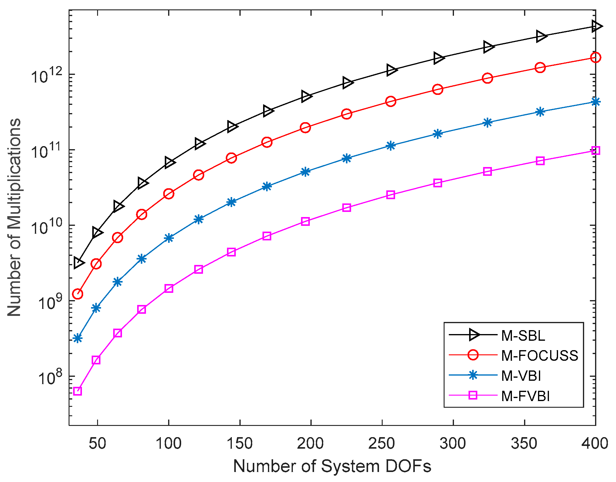
4. Computational Complexity Analysis

The computational complexity of the proposed algorithm is investigated via the number of complex multiplications, and the lower-order terms of the multiplication are omitted. In the proposed M-FVBI-STAP algorithm, the computational complexity is related to the dimension of Ψ M N × P . P is the number of selected atoms that is assumed to be twice the rank of the clutter. The most computational part of M-VBI-STAP is Equation (24). Table 1 shows the computational complexity of different approaches. T S B L , T F O C U S S , T V B I and T F V B I represent the number of iterations of M-FOCUSS-STAP, M-SBL-STAP [24], M-VBI-STAP and M-FVBI-STAP. The results are plotted in Figure 2. As the number of system DOFs increases, it is observed that the computational complexity of the M-VBI-STAP is lower than M-SBL-STAP and M-FOCUSS-STAP. Compared to M-VBI-STAP, M-FVBI-STAP can improve computational efficiency.

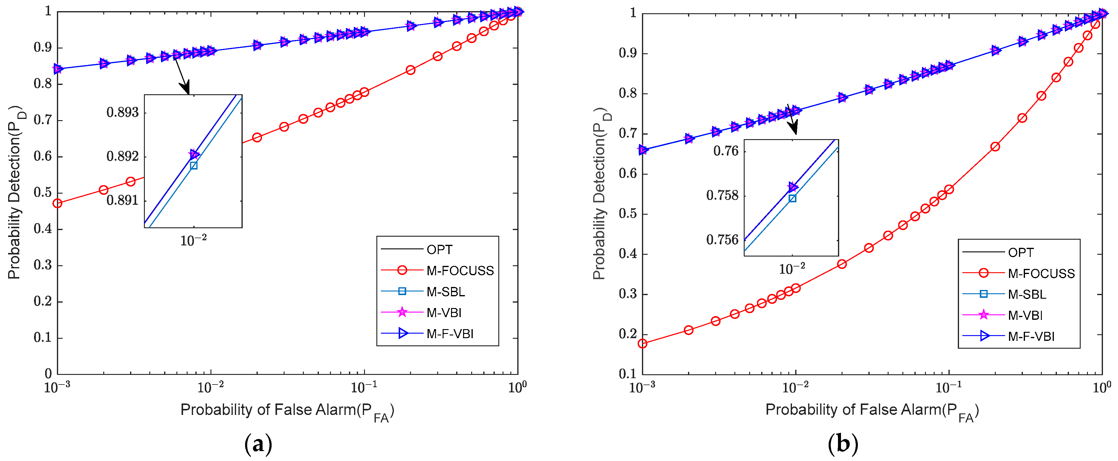
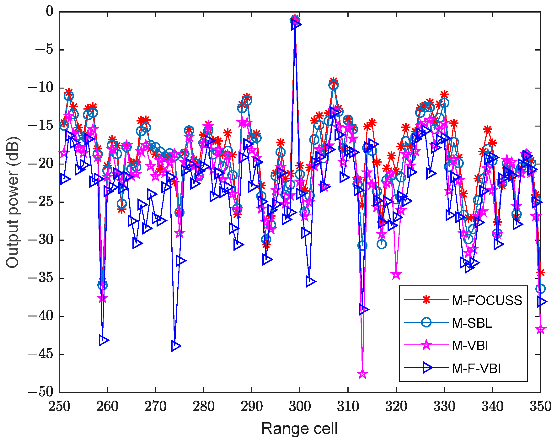
5. Numerical Experiments
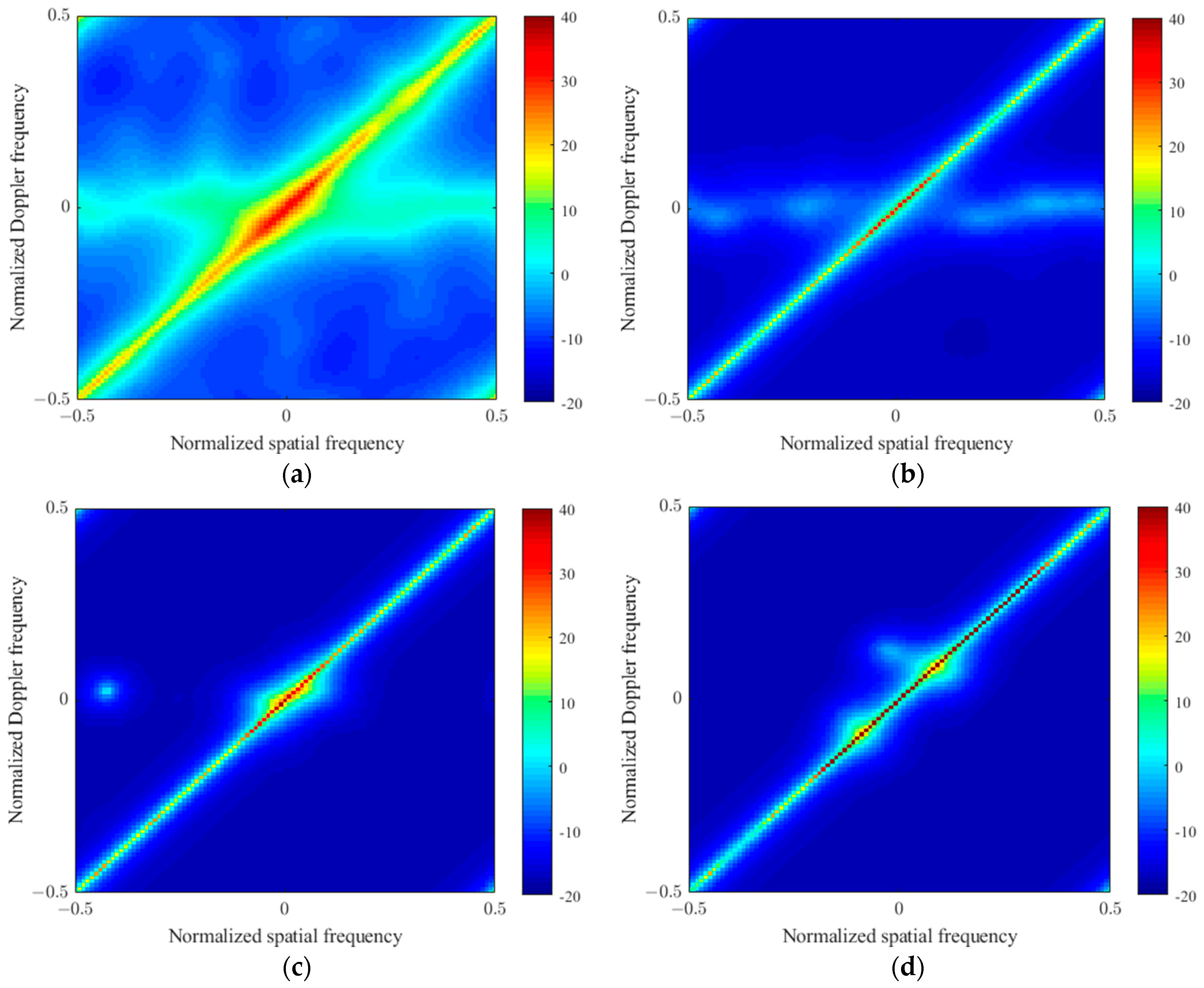
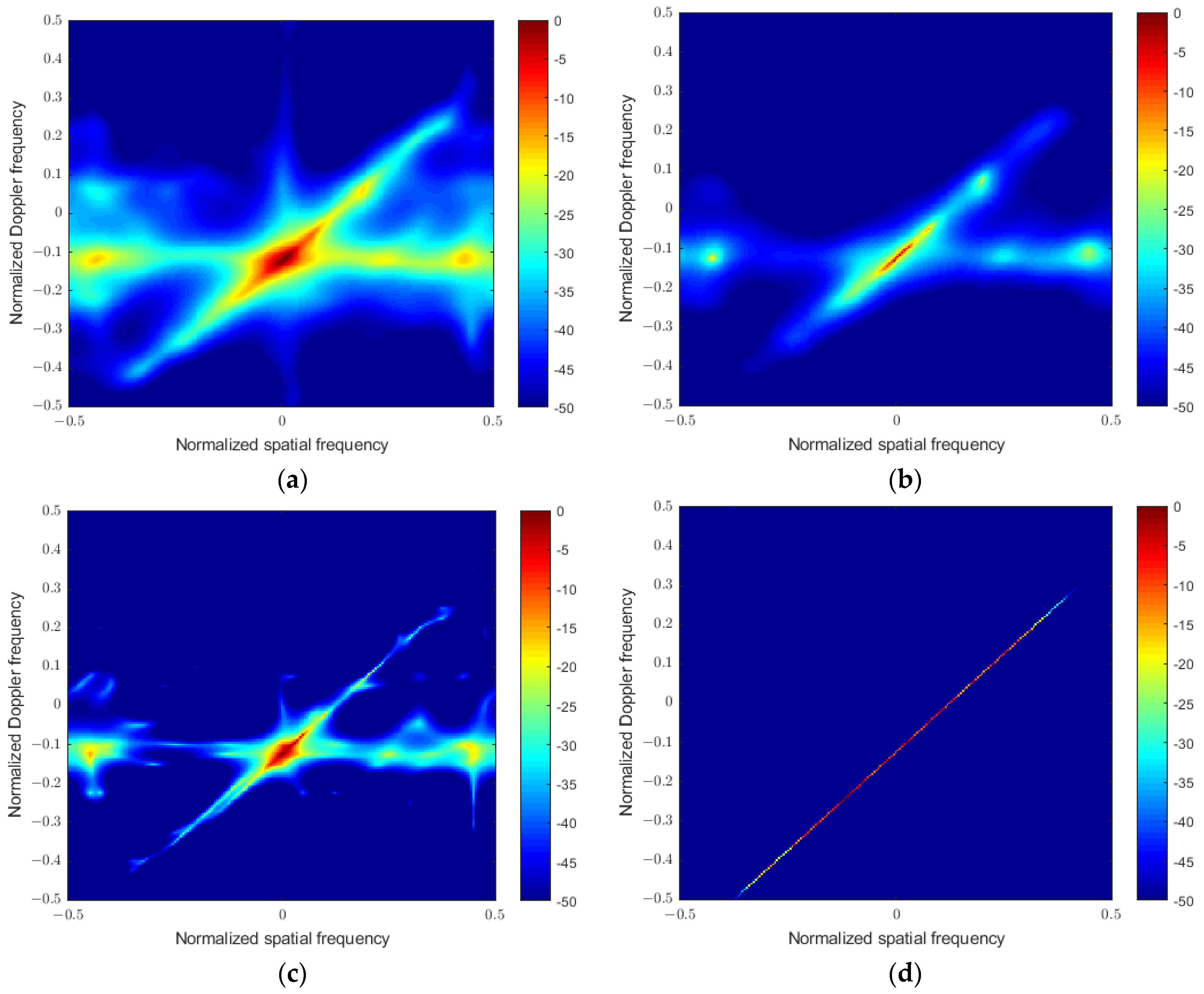
5.1. Simulated Data

In this section, numerical experiments are conducted to illustrate the STAP and target detection performance of the proposed algorithm on simulated data. The main parameters of the simulations are listed in Table 2 and ρ s = ρ d = 5 . For comparison, M-SBL-STAP and M-FOCUSS-STAP are presented. In addition, the optimal STAP with known CNCM and diagonal loading SMI-STAP (LSMI-STAP) are also included. The results are averaged over 100 Monte Carlo trials, and the number of training samples used in all experiments is ten. To measure the performance of clutter suppression, the improvement factor (IF) and signal-to-interference plus noise ratio (SINR) loss are used, which are denoted as
I F = | w H a t | w H R c + n w t r ( R c + n ) a t H a t
L S I N R = σ 2 M N | w H a t | 2 w H R c + n w
The STAP performance in terms of Capon spectra is first investigated. Figure 3a plots the optimal spectrum with known CNCM. From Figure 3b–f, it can be noted that the estimation results of the proposed M-FVBI, M-VBI algorithm, and M-SBL-STAP are close to the optimal spectrum. In addition, the spectra of M-FOCUSS-STAP have an extension in the main-lobe region. It can also be seen that the spectrum is inaccurate when estimated by LSMI-STAP due to the lack of training samples. Figure 4 plots the Capon spectra with gain–phase (GP) error, which are set as 0.05 and 2°. Compared to Figure 3a, it can be seen that the results of the proposed M-FVBI, M-VBI algorithm, and M-SBL-STAP are close to the optimal spectrum.
Then, the IF curves of different approaches against the normalized Doppler frequency in the main beam direction are presented in Figure 5. It is shown in Figure 5 that M-FVBI-STAP, M-VBI-STAP, and M-SBL-STAP have a similar performance, which is near the optimal performance. In the main-lobe area, the curves of the M-FOCUSS-STAP are broader than others.
For the next experiment, the average SINR loss curves versus the number of training samples are plotted in Figure 6, which were calculated as the mean SINR loss curves for f d = ( 0.5 , 0.1 ) ( 0.1 , 0.5 ) . It can be seen from Figure 6 that all the approaches achieved a relatively stable performance when the number of training samples was more than three, and the stable performance of M-FOCUSS-STAP was worse than others. The M-VBI-STAP and M-FVBI-STAP had the best performance.
For a clearer illustration, the target detection performance of the proposed algorithm was accessed. According to [41], the probability of detection (PD) versus the probability of false alarm (PFA) is defined as
P D = P F A 1 1 + ξ
where ξ is the output signal-to-clutter-plus-noise ratio (SCNR). We set the target located in the main beam direction.
As shown in Figure 7, the receiver operating characteristics (ROC) (i.e., PD versus PFA) are plotted with the target signal-to-noise ratio (SNR), 0 dB and −4 dB, respectively. The normalized Doppler frequency is f d = 0.1 . It can be seen that the detection performances of the M-SBL-STAP, M-VBI-STAP, and M-FVBI-STAP are close to optimal. Another notable result is that the detection performances increased with the growth of the SNR value. The ROC results with f d = 0.3 are shown in Figure 8. The detection performance increased compared to f d = 0.1 . In both cases, M-VBI-STAP and M-FVBI-STAP are considered optimal.
Finally, the average running time for different cases is summarized in Table 3. The experiments were conducted by MATLAB 2017b on the computer equipped with Intel(R) Xeon(R) E5-2620 CPU @ 2.10Hz 2.10Hz and 64G RAM. It was found that the average running time of M-VBI-STAP was less than M-SBL-STAP. M-FVBI-STAP significantly accelerated the average running time.

5.2. Measured Data

In this subsection, the performance of the proposed algorithm is accessed with publicly available data from Multi-Channel Airborne Radar Measurement (MCARM) data. [42]. The airborne radar of the MCARM can be viewed as side looking. In CPI data, the number of coherent pluses, array elements, and range cells are 128, 22, and 630, respectively. For 12 pluses, data from the first space channels are selected for experimental analysis. There is a target added in the 320th range cell. Since the first 150 range cells cannot be used, the clutter power spectrum shown in Figure 9 was estimated using ten training samples selected from ye 151st range cell to the 630th range cell. It can be seen that all the approaches can recover the clutter ridge. The spectra of the M-FOCUSS-STAP have an extension in the main-lobe region. In addition, M-FVBI-STAP estimated CNCM by selecting the atoms. Thus, the clutter ridge of the M-FVBI-STAP is concentrated on a diagonal line.
The STAP output power from the 280th range cell to the 360th range cell is depicted in Figure 10. The generalized inner product (GIP) method [43] was used to select ten range cells of the twenty range cells around the CUT as the training samples. Additionally, four range cells on each side of the CUT were chosen as the guard cells. It can be observed that all algorithms clearly detected the target. To further illustrate the detection performance, the output signal to clutter plus noise ratio (SCNR) was calculated at the target range cell. The result corresponding to the algorithms is listed in Table 4. The proposed algorithm clearly had the best detection performance of all approaches.

6. Conclusions

In this paper, the framework of VBI into the STAP algorithm has been developed, which can improve the convergence speed compared to SBL. Due to the heavy computational burden caused by the matrix inverse operation, a fast iterative algorithm was derived. The numerical results of the simulated data and measured data demonstrate that the proposed algorithm has superior STAP and target detection performance and can effectively reduce computational complexity. VBI still belongs to SR algorithms, which require dictionary construction. When the grid mismatch exists, the performance of VBI decreases. The direction for future research is mitigating the grid mismatch effect on SR-STAP.

Author Contributions

Conceptualization, T.W.; methodology, X.Z.; validation, X.Z. and D.W.; writing—original draft preparation, X.Z.; writing—review and editing, D.W.; visualization, X.Z. and D.W.; supervision, T.W.; project administration, T.W. All authors have read and agreed to the published version of the manuscript.

Funding

This research was funded by the National Key R&D Program of China, grant number 2021YFA1000400.

Data Availability Statement

Not applicable.

Conflicts of Interest

The authors declare no conflict of interest.

Appendix A

(1)
Update formulas for removing the atoms.
We define the Σ ¯ j as
Σ ¯ j = ( δ Ψ j ¯ H Ψ j ¯ + d i a g ( α j ¯ ) δ Ψ j ¯ H s j δ s j H Ψ j ¯ δ s j H s j ) 1
where Ψ j ¯ and α j ¯ are the dictionary and sparse coefficient by removing s j and λ j . Using the block matrix inversion, Equation (A5) is equivalent to
Σ ¯ j = ( Σ ˜ + γ j δ 2 Σ ˜ Ψ j ¯ H s j s j H Ψ j ¯ Σ ˜ γ j δ Σ ˜ Ψ j ¯ H s j γ j δ s j H Ψ j ¯ Σ ˜ γ j )
where γ j = ( δ s j H s j δ 2 s j H Ψ j ¯ Σ ˜ Ψ j ¯ H s j ) 1 , Σ ˜ represents the variance of the current model,
Σ ˜ = ( δ Ψ j ¯ H Ψ j ¯ + d i a g ( α j ¯ ) ) 1 = [ Σ Σ e j e j H Σ e j H Σ e j ] j ¯ j ¯
and the mean of the model is
μ ˜ l = [ μ l Σ e j e j H μ l e j H Σ e j ] j ¯
Then, ς j and ρ j , l can be updated as
ς j = ( δ s j H s j δ 2 s j H Ψ j ¯ Σ ˜ Ψ j ¯ H s j ) 1
ρ j , l = δ ς j s j H x l δ 2 ς j s j H Ψ j ¯ Σ ˜ Ψ j ¯ H x l
(2)
Update the formulas of re-estimating atoms.
The variance of the current model is
Σ ˜ = Σ κ Σ e j e j H Σ
where κ = λ j e j H α 1 + ( e j H Σ e j ) ( λ j e j H α ) . The mean of the model is
μ ˜ l = μ l κ e j H Σ e j e j H μ l
Then, ς j and ρ j , l can be updated as
ς j = ( δ s j H s j δ 2 s j H Ψ Σ ˜ Ψ H s j ) 1
ρ j , l = δ ς j s j H x l δ 2 ς j s j H Ψ Σ ˜ Ψ H x l
(3)
Update the formulas for adding atoms.
The variance of the current model can be defined as
Σ ˜ = ( δ Ψ H Ψ + d i a g ( α ) δ Ψ H s j δ s j H Ψ δ s j H s j ) 1
where s j Ψ . Using block matrix inversion, Equation (A5) is equivalent to
Σ ˜ = ( Σ + γ j δ 2 Σ Ψ H s j s j H Ψ Σ γ j δ Σ Ψ H s j γ j δ s j H Ψ Σ γ j )
where γ j = ( δ s j H s j + λ j δ 2 s j H Ψ Σ Ψ H s j ) 1 . The mean of the model is
μ ˜ l = δ Σ ˜ Ψ j H x l
where Ψ j = [ Ψ , s j ] . Then, ς j and ρ j , l can be updated as
ς j = ( δ s j H s j + λ j δ 2 s j H Ψ j Σ ˜ Ψ j H s j ) 1
ρ j , l = δ ς j s j H x l δ 2 ς j s j H Ψ j Σ ˜ Ψ j H x l

References

  1. Ward, J. Space-Time Adaptive Processing for Airborne Radar; Technical Report; MIT Lincoln Laboratory: Lexington, KY, USA, 1994. [Google Scholar]
  2. Brennan, L.E.; Reed, L.S. Theory of adaptive radar. IEEE Trans. Aerosp. Electron. Syst. 1973, 9, 237–251. [Google Scholar] [CrossRef]
  3. Smith, S.T. Adaptive radar. In Wiley Encyclopedia of Electrical and Electronics Engineering; Wiley: Hoboken, NJ, USA, 2001. [Google Scholar]
  4. Melvin, W.L. Space-time adaptive processing and adaptive arrays: Special collection of papers. IEEE Trans. Aerosp. Electron. Syst. 2000, 36, 508509. [Google Scholar] [CrossRef]
  5. Klemm, R. Principles of Space-Time Adaptive Processing; The Institution of Electrical Engineers: London, UK, 2006. [Google Scholar]
  6. Reed, L.S.; Mallet, J.D.; Brennan, L.E. Rapid convergence rate in adaptive arrays. IEEE Trans. Aerosp. Electron. Syst. 1974, 10, 853–863. [Google Scholar] [CrossRef]
  7. Pallotta, L.; Farina, A.; Smith, S.T.; Giunta, G. Phase-only space-time adaptive processing. IEEE Access 2021, 9, 147250–147263. [Google Scholar] [CrossRef]
  8. Haimovich, A.M.; Bar-Ness, Y. An eigenanalysis interference canceller. IEEE Trans. Signal Process. 1991, 39, 76–84. [Google Scholar] [CrossRef]
  9. Hua, Y.; Nikpour, M.; Stoica, P. Optimal reduced rank estimation and filtering. IEEE Trans. Signal Process. 2001, 49, 457–469. [Google Scholar]
  10. Goldstein, J.S.; Reed, I.S.; Scharf, L.L. A multistage representation of the Wiener filter based on orthogonal projections. IEEE Trans. Inf. Theory 1998, 44, 2943–2959. [Google Scholar] [CrossRef]
  11. Haimovich, A. The eigencanceler: Adaptive radar by eigenanalysis methods. IEEE Trans. Aerosp. Electron. Syst. 1996, 32, 532–542. [Google Scholar] [CrossRef]
  12. Wang, H.; Cai, L. On adaptive spatial-temporal processing for airborne surveillance radar systems. IEEE Trans. Aerosp. Electron. Syst. 1994, 30, 660–670. [Google Scholar] [CrossRef]
  13. Klemm, R. Adaptive airborne MTI: An auxiliary channel approach. IEEE Proc. F Commun. Radar Signal Process. 1987, 134, 269–276. [Google Scholar] [CrossRef]
  14. DiPietro, R.C. Extended factored space-time processing for airborne radar systems. Signals Syst. Comput. 1992, 1, 425–430. [Google Scholar]
  15. Zhang, W.; He, Z.; Li, J.; Liu, H.; Sun, Y. A method for finding best channels in beam-space post-Doppler reduced-dimension STAP. IEEE Trans. Aerosp. Electron. Syst. 2014, 50, 254–264. [Google Scholar] [CrossRef]
  16. Lin, X.; Blum, R.S. Robust STAP algorithms using prior knowledge for airborne radar applications. Signal Process. 1999, 79, 273–287. [Google Scholar] [CrossRef]
  17. Guerci, J.R.; Baranoski, E.J. Knowledge-aided adaptive radar at DARPA: An overview. IEEE Signal Process. 2006, 23, 41–50. [Google Scholar] [CrossRef]
  18. Gerlach, K.; Picciolo, M.L. Airborne/spacebased radar STAP using a structured covariance matrix. IEEE Trans. Aerosp. Electron. Syst. 2003, 39, 269–281. [Google Scholar] [CrossRef]
  19. Steiner, M.; Gerlach, K. Fast converging adaptive processor or a structured covariance matrix. IEEE Trans. Aerosp. Electron. Syst. 2000, 36, 1115–1126. [Google Scholar] [CrossRef]
  20. Kang, B.; Monga, V.; Rangaswamy, M. Rank-constrained maximum likelihood estimation of structured covariance matrices. IEEE Trans. Aerosp. Electron. Syst. 2014, 50, 501–515. [Google Scholar] [CrossRef]
  21. De Maio, A.; De Nicola, S.; Landi, L.; Farina, A. Knowledge-aided covariance matrix estimation: A MAXDET approach. IET Radar Sonar Navig. 2009, 3, 341–356. [Google Scholar] [CrossRef]
  22. Aubry, A.; De Maio, A.; Pallotta, L. A geometric approach to covariance matrix estimation and its applications to radar problems. IEEE Trans. Signal Process. 2017, 66, 907–922. [Google Scholar] [CrossRef]
  23. Sun, K.; Zhang, H.; Li, G.; Meng, H.D.; Wang, X.Q. A novel STAP algorithm using sparse recovery technique. IEEE Int. Geosci. Remote Sens. Symp. 2009, 1, 3761–3764. [Google Scholar]
  24. Sun, K.; Meng, H.; Wang, Y. Direct data domain STAP using sparse representation of clutter spectrum. Signal Process. 2011, 91, 2222–2236. [Google Scholar] [CrossRef]
  25. Yang, Z.; Li, X.; Wang, H.; Jiang, W. On clutter sparsity analysis in space–time adaptive processing airborne radar. IEEE Geosci. Remote. Sens. Lett. 2013, 10, 1214–1218. [Google Scholar] [CrossRef]
  26. Cotter, S.F.; Rao, B.D.; Engan, K.; Kreutz-Delgado, K. Sparse solutions to linear inverse problems with multiple measurement vectors. IEEE Trans. Signal Process. 2005, 53, 2477–2488. [Google Scholar] [CrossRef]
  27. Tropp, J.; Gilbert, A. Signal recovery from random measurements via orthogonal matching pursuit. IEEE Trans. Inf. Theory 2007, 53, 4655–4666. [Google Scholar] [CrossRef]
  28. Gorodnitsky, I.; Rao, B. Sparse signal reconstruction from limited data using FOCUSS a re-weighted minimum norm algorithm. IEEE Trans. Signal Process. 1997, 45, 600–616. [Google Scholar] [CrossRef]
  29. Wu, Q.; Zhang, Y.; Amin, M.G.; Himed, B. Space-time adaptive processing and motion parameter estimation in multistatic passive radar using sparse Bayesian learning. IEEE Trans. Geosci. Remote. Sens. 2016, 54, 944–957. [Google Scholar] [CrossRef]
  30. Duan, K.Q.; Wang, Z.T.; Xie, W.C.; Chen, H.; Wang, Y.L. Sparsity-based STAP algorithm with multiple measurement vectors via sparse Bayesian learning strategy for airborne radar. IET Signal Process. 2017, 11, 544–553. [Google Scholar] [CrossRef]
  31. Wang, Z.T.; Xie, W.C.; Duan, K.Q. Clutter suppression algorithm base on fast converging sparse Bayesian learning for airborne radar. Signal Process. 2017, 130, 159–168. [Google Scholar] [CrossRef]
  32. Tzikas, D.; Likas, A.; Galatsanos, N. The variational approximation for Bayesian inference. IEEE Signal Process. 2008, 25, 131–146. [Google Scholar] [CrossRef]
  33. Guo, K.; Zhang, L.; Li, Y.; Zhou, T.; Yin, J. Variational Bayesian Inference for DOA Estimation under Impulsive Noise and Non-uniform Noise. IEEE Trans. Aerosp. Electron. Syst. 2023. [Google Scholar] [CrossRef]
  34. Shutin, D.; Buchgraber, T.; Kulkarni, S.; Poor, H. Fast variational sparse Bayesian learning with automatic relevance determination for superimposed signals. IEEE Trans. Signal Process. 2011, 95, 6257–6261. [Google Scholar] [CrossRef]
  35. Zhou, S.; Xu, A.; Tang, Y.; Shen, L. Fast Bayesian inference of reparameterized gamma process with random effects. IEEE Trans. Reliab. 2023, in press. [Google Scholar] [CrossRef]
  36. Turlapaty, A.C. Variational Bayesian estimation of statistical properties of composite gamma log-normal distribution. IEEE Trans. Signal Process. 2020, 68, 6481–6492. [Google Scholar] [CrossRef]
  37. Yuan, W.; Wei, Z.; Yuan, J.; Ng, D.W.K. A Simple Variational Bayes Detector for Orthogonal Time Frequency Space (OTFS) Modulation. IEEE Trans. Veh. Technol. 2020, 69, 7976–7980. [Google Scholar] [CrossRef]
  38. Bishop, C. Pattern Recognition and Machine Learning; Springer: New York, NY, USA, 2006. [Google Scholar]
  39. Thomas, B. Variational Sparse Bayesian Learning: Centralized and Distributed Processing; Graz University of Technology: Graz, Austria, 2013. [Google Scholar]
  40. Tipping, M.; Faul, A. Fast marginal likelihood maximization for sparse Bayesian models. In Proceedings of the Ninth International Workshop on Artificial Intelligence and Statistics, Key West, FL, USA, 3–6 January 2003; pp. 276–283. [Google Scholar]
  41. Robey, F.C.; Fuhrmann, D.; Kelly, E.; Nitzberg, R. A CFAR adaptive matched filter detector. IEEE Trans. Aerosp. Electron. Syst. 1992, 28, 208–216. [Google Scholar] [CrossRef]
  42. Wu, Y.; Wang, T.; Wu, J. A knowledge-aided space time adaptive processing based on road network data. J. Electron. Sci. Technol. 2015, 37, 613–618. [Google Scholar]
  43. Melvin, W.L.; Wicks, M.C. Improving practical space-time adaptive radar. In Proceedings of the 1997 IEEE National Radar Conference, Syracuse, NY, USA, 13–15 May 2005; pp. 48–53. [Google Scholar]
Figure 1. Bayesian graphical model.
Remotesensing 15 04334 g001
Figure 2. Computational complexity versus the number of system DOFs.
Remotesensing 15 04334 g002
Figure 3. Capon spectra of different approaches. (a) Capon spectrum estimated by known CNCM; (b) Capon spectrum estimated by LSMI-STAP; (c) Capon spectrum estimated by M-FOCUSS-STAP; (d) Capon spectrum estimated by M-SBL-STAP; (e) Capon spectrum estimated by M-VBI-STAP; (f) Capon spectrum estimated by the M-FVBI-STAP.
Remotesensing 15 04334 g003aRemotesensing 15 04334 g003b
Figure 4. Capon spectra of different approaches with GP error. (a) Capon spectrum estimated by M-FOCUSS-STAP; (b) Capon spectrum estimated by M-SBL-STAP; (c) Capon spectrum estimated by M-VBI-STAP; (d) Capon spectrum estimated by the M-FVBI-STAP.
Remotesensing 15 04334 g004
Figure 5. IF against the normalized Doppler frequency.
Remotesensing 15 04334 g005
Figure 6. Average IF against the number of training samples.
Remotesensing 15 04334 g006
Figure 7. Receiver operating characteristics with f d = 0.1 . (a) SNR = 0 dB; (b) SNR = −4 dB.
Remotesensing 15 04334 g007
Figure 8. Receiver operating characteristics with f d = 0.3 . (a) SNR = 0 dB; (b) SNR = −4 dB.
Remotesensing 15 04334 g008
Figure 9. Estimated clutter power spectra of different approaches. (a) Capon spectrum estimated by M-FOCUSS-STAP; (b) Capon spectrum estimated by M-SBL-STAP; (c) Capon spectrum estimated by M-VBI-STAP; (d) Capon spectrum estimated by the M-FVBI-STAP.
Remotesensing 15 04334 g009
Figure 10. STAP output power versus range cells.
Remotesensing 15 04334 g010
Table 1. Computational complexity.
AlgorithmComputational Load
M-SBL o ( ( ( M N ) 3 + 2 K ( M N ) 2 + K 2 M N + K M N L ) T S B L )
M-FOCUSS o ( ( ( M N ) 3 + 2 ( M N ) 2 K + M N L K ) T F O C U S S )
M-VBI o ( ( ( M N ) 3 + 2 K ( M N ) 2 + K 2 M N + K M N L ) T V B I )
M-FVBI o ( ( M N K + M N L + 4 M N K P + M N L P ) T F V B I )
Table 2. Parameters of radar system.
ParameterValueUnit
Number of elements8/
Number of pulses8/
Wavelength0.3m
Bandwidth2.5MHz
Height of platform150m/s
Velocity of platform9000m
Pulse repetition frequency (PRF)2000Hz
Clutter to noise ratio (CNR)40dB
Table 3. The average running time (second).
AlgorithmsRunning Time
M-SBL34.88 s
M-FOCUSS11.16 s
M-VBI3.70 s
M-FVBI0.05 s
Table 4. The output SCNR (dB).
AlgorithmsResults
M-SBL16.43 dB
M-FOCUSS16.89 dB
M-VBI18.86 dB
M-FVBI19.58 dB
Disclaimer/Publisher’s Note: The statements, opinions and data contained in all publications are solely those of the individual author(s) and contributor(s) and not of MDPI and/or the editor(s). MDPI and/or the editor(s) disclaim responsibility for any injury to people or property resulting from any ideas, methods, instructions or products referred to in the content.

