Abstract
The effectiveness indicator system of remote sensing satellites includes various satellites capabilities. Effectiveness evaluation is the process of calculating these indicators in the digital world, involving many different physical parameters of multiple subsystems. Model-based simulation statistics method is the mainstream approach of effectiveness evaluation, and digital twin is currently the most advanced modeling method for simulation. The satellite digital twin model has the characteristics of multi-dynamic, multi-spatial scale and multi-physics field coupling, which gives rise to challenges related to the stiff problem of ordinary differential equations and multi-scale problem of partial differential equations to the calculation process of indicators. It is difficult to solve these problems by breakthroughs in numerical solution methods. This paper uses the sparsity of the satellite system to group each indicator of the effectiveness evaluation indicator system according to the change period. The satellite system model is decomposed into multiple modules according to the composition and structure, and a series of models with different simulation fidelity are established for each module. The optimization schemes for selecting model granularity when calculating indicators by group is given. Simulation results show that this approach considers the coupling between systems, grasps the main contradiction of indicator calculation and overcomes the loss of indicator accuracy caused by the separate calculation of each subsystem under the neglect of coupling in the traditional method. Additionally, it avoids the difficulty in numerical calculation caused by coupling, while simultaneously balancing the accuracy and efficiency of the model simulations.
1. Introduction
Remote sensing satellites are a type of satellite that utilizes optical or microwave technology to collect information about the ground or air targets. They have numerous applications in areas such as agriculture, forestry, marine, land management, environmental protection, weather forecasting, and military operations [1,2,3,4,5,6,7,8]. To create a comprehensive remote sensing satellite system, it is crucial to evaluate the effectiveness of these satellites [9,10]. A rational and scientific effectiveness evaluation process can serve as a valuable reference for the requirements demonstration and development of remote sensing satellites. It is conducive to optimizing the design of remote sensing satellite and improving the capability of task execution [11,12].
There are several methods for effectiveness evaluation, and the simulation statistics methods have proven to be advantageous for the quantitative evaluation of complex problems [13]. Simulation statistics methods are used to evaluate effectiveness through modeling and simulation. After many years of development, this field has mainly divided into two directions: functional direct modeling and principle modeling [14]. Functional direct modeling involves building models based on the functions of the object being evaluated, resulting in a simple approach. However, this method often leads to high uncertainty and low accuracy in the evaluation. In contrast, principle modeling refers to build models through the mathematical analysis of the operating principles of the system [15,16]. Computational resource requirements are high, but high-fidelity simulations of modeling can be accomplished [17]. In 1994, Hughes and Loral Company in the United States(US) pioneered the use of dynamic simulation technology in satellite engineering by dividing subsystems into the structure, power, thermal control, Telemetry Tracking and Command(TTC), propulsion, attitude control, and payload. They also utilized model sharing to facilitate the exchange of work results among personnel in different positions [18]. In 1997, the US Department of Defense proposed the concept of virtual prototyping (VP), which aimed to map digital systems to physical systems completely [19]. In 2003, GRIEVES introduced the concept of Digital Twin (DT) and, in collaboration with the Air Force Research Laboratory, defined it as a simulation process that utilizes mathematical models, sensor updates, history operation data and integrates multidisciplinary, multi-physical quantities, and multiple scales and probabilities. This process aimed to achieve a complete mapping of physical systems in the digital world, reflecting the full life cycle of real physical systems [20]. Considering multi-dynamic, multi-spatial scale and multi-physics coupling in the whole life cycle of the system is the core feature of DT modeling. The concept of DT has since been widely accepted and recognized as the cornerstone of the new industrial revolution [21].
Effectiveness evaluation reflects the overall system capability of remote sensing satellites. The indicator system is a set. Some indicators are system-wide, such as mass, cost-effectiveness ratio, etc. [22]. Some indicators are decomposed by satellite components, focusing on satellite subsystem capabilities. Wang Xiji [23] established an evaluation indicator system for the functions and performance of commonly used satellite platforms and payloads, which reflects the system capabilities of satellites relatively completely. In this indicator system, the remote sensing payload subsystem indicators include parameters such as time coverage, payload data rate, and image signal-to-noise ratio (SNR). The attitude and orbit control indicators include attitude measurement accuracy, attitude pointing accuracy, and attitude stability accuracy. For the power subsystem’s power consumption, the maximum output power of the solar array and other indicators are used to assess the performance. The thermal control subsystem indicators include the equilibrium temperature of the entire satellite and the temperature of typical devices. The propulsion subsystem indicators include specific impulse and propellant extrusion efficiency. The TTC subsystem indicators include TTC time coverage and TTC data transmission rate. It should be pointed out that although it can be classified by subsystem, each indicator shows the performance of this subsystem in a specific system and environment, and is the ability of this subsystem and the environment outside the system to interact with each other. For instance, when calculating attitude measurement accuracy, the error characteristics of the gyroscope are significantly influenced by the rotor shaft temperature. Any changes in external temperature will directly impact the measurement accuracy. Therefore, it is imperative to include temperature model to accurately reflect the state changes of the gyroscope [24]. Momentum wheels also exhibit similar characteristics, where the friction force on their shaft is influenced by temperature and affects the control torque output [25]. Simply establishing a model of this subsystem cannot reflect the relationship between this subsystem and other subsystems and the environment. Therefore, when evaluating these indicators, it is necessary to establish a model of a complete satellite system and environment to reflect the relationship between each subsystem and the environment. Without considering coupling, it cannot accurately reflect the core characteristics of digital satellites.
The challenge of digital satellite coupling modeling is that the state of the satellite has multiple dynamics and multiple spatial scales [26]. Multi-dynamic refers to the inconsistency of the change cycle of satellite state parameters. When using the attitude and orbit control component-level model to calculate the attitude and orbit control indicators, the simulation step size is more appropriate in milliseconds [27]. In an attempt to accurately calculate power indicators, a detailed model of the power supply system is necessary, which requires data on the sunlit and Earth shadow areas of the satellite, as well as data on several orbital periods. The charging and discharging processes of the power supply are relatively slow, requiring simulation step size measured in seconds [28]. Conversely, when calculating thermal control indicators, a more detailed thermal control mesh must be established, the periods of thermal decay effects on components are long and data over extended periods of several months or even years is necessary for indicator calculation, with simulation step size measured in hours or days [29]. It is possible to evaluate each indicator independently with each subsystem model, but to form a complete system model, it is necessary to couple all subsystem models such as the attitude and orbit control, power and thermal control together for calculation. At this time, it is difficult to choose the simulation step size. The multi-spatial scale problems is the same. Different problems involve different spatial scales. It is easy to choose the size of the finite element if it is solved independently, but if considering the coupling, the size of the finite element varies greatly, which causes difficulties to solve the partial differential equation.
A model is a simplified representation of real-world objects, and the depth of human understanding of real things is endless. For the specific problems to be studied, infinitely fine models are not necessary, as long as they meet the needs of the research problems. When evaluating the effectiveness of remote sensing satellites, it is not to adjust the model accuracy of each subsystem synchronously with the same accuracy, but to arrange the accuracy of the simulation model of each subsystem according to the indicators to be evaluated and the coupling degree of each subsystem. A fine-grained model with high precision is selected for key subsystems, and a coarse-grained model with low precision is selected for subsystems with relatively low correlation. When calculating attitude and orbit control indicators, instead of only building a fine-grained attitude and orbit control model and ignoring other subsystem models, it is appropriate to coarsen the granularity of the power, thermal control, and telemetry subsystems. When calculating the thermal control indicators, the division of the thermal meshes needs to be detailed enough, the model of the thermal control component should be refined, and the granularity of other subsystems should be appropriately coarsened. Additionally, for the power, thermal control, propulsion, TTC, and payload subsystems, it is necessary to refine their models based on their specific goals while coarsening the models of other systems.
To address these issues, this paper proposes a multi-granularity model effectiveness evaluation method for remote sensing satellites. This paper classifies indicators of the effectiveness evaluation indicator system according to the change period, establishes simulation models with different simulation fidelity for each subsystem. For each category of indicators, a satellite model with different granularities is selected, and a multi-granularity satellite effectiveness evaluation scheme is obtained.
The rest of this paper is organized as follows. Section 2 begins with a mathematical description of the evaluation indicators, followed by multi-granularity modeling. In Section 3, the model granularity corresponding to the three types of indicators is described. In Section 4, a discussion of the simulation case and results analysis is provided. Lastly, Section 5 concludes this paper and describes future work.
2. A Mathematical Description of Remote Sensing Satellite Effectiveness Evaluation Problem
2.1. Typical Satellite Effectiveness Evaluation Indicator
Time resolution refers to the minimum time step of the simulation process. The changes in physical quantities and the simulation duration required to calculate indicators will impact the selection of time resolution. In this section, the typical effectiveness indicators with classical characteristics are filtered from commonly used indicators, and are classified according to time resolution.
2.1.1. Millisecond-Level Time Resolution Indicator
(1) Attitude measurement accuracy
The measurement accuracy of the three-axis attitude is equal to the maximum absolute value of the difference between the attitude angle and the reference attitude angle, and the real dynamic attitude angle error at all times.
where , , and represent the measurement accuracy of roll angle, pitch angle, and yaw angle, , and represent the roll angle, pitch angle, and yaw angle measured by the sensor, , and are the real dynamic roll angle, pitch angle, and yaw angle.
(2) Attitude pointing accuracy
The three-axis pointing accuracy is equal to the absolute value of the difference between the expected target attitude angle and the three-axis stable attitude angle.
where , , and represent pointing accuracy of roll angle, pitch angle, and yaw angle.
(3) Attitude stable accuracy
The three-axis stability accuracy is equal to the difference between the expected target attitude angular velocity and the three-axis stable attitude angular velocity.
where , , and represent stable accuracy of roll angular velocity, pitch angular velocity, and yaw angular velocity.
2.1.2. Second-Level Time Resolution Indicator
(1) Bus power supply performance
(2) Output power of solar array
(3) Maximum output power of solar array
The maximum output power of a solar array over some time
(4) Maximum discharge depth of the battery
(5) Efficiency of propellant
(6) Specific impulse
is the specific impulse of propellant, the total impulse is as follows
2.1.3. Day-Level Time Resolution Indicator
(1) Subsystem thermal power
The thermal power of the thermal control system is equal to the sum of the thermal power of all devices of the thermal control subsystem
where is thermal power of the thermal control subsystem, represents the devices of the thermal control subsystem, is device thermal power.
For any device (the number is the temperature at a certain time point can be obtained from the thermal control subsystem model, calculate the temperature at all time points to obtain the minimum temperature and maximum temperature .
(2) Node temperature
By calculating the temperature at all time points of all hot nodes on the satellite, the equilibrium temperature , minimum temperature , and maximum temperature of the entire satellite can be obtained. The formula is as follows,
where represents the total number of thermal nodes, is the temperature of the node , and is the time point.
(3) Payload time coverage
The number of coverage times is equal to the number of coverage periods in the entire simulation time.
where is the simulation start time, is the time point of the th step of the simulation start, is the time point of simulation end time point, is switching identification from noncoverage time period to coverage period, is the time point of noncoverage time, and is the time point of observing time.
The total coverage time is equal to the sum of each coverage time
The coverage rate on target time is
The average coverage time can be calculated by dividing the total coverage time by the number of coverage times.
(4) Discovery probability [30]
is the total number of tasks found in an orbital period after all targets are lost
where is each lost time of the target and is the last recent discovery time.
(5) Discovery response time [30]
(6) Payload data rate [31]
(7) Coverage of telemetry and command
The number of coverage times is equal to the number of coverage time intervals in the overall simulation duration.
where is the simulation start time, is the time point of the th step of the simulation start, is the time point of simulation end time point, is switching identification from noncoverage period to the coverage period, is the time point of noncoverage time, and is the time point of observing time.
The total coverage time is equal to the sum of each coverage time
The coverage rate on target time is
The average coverage time can be calculated by dividing the total coverage time by the number of coverage times.
2.2. Multi-Granularity Modeling
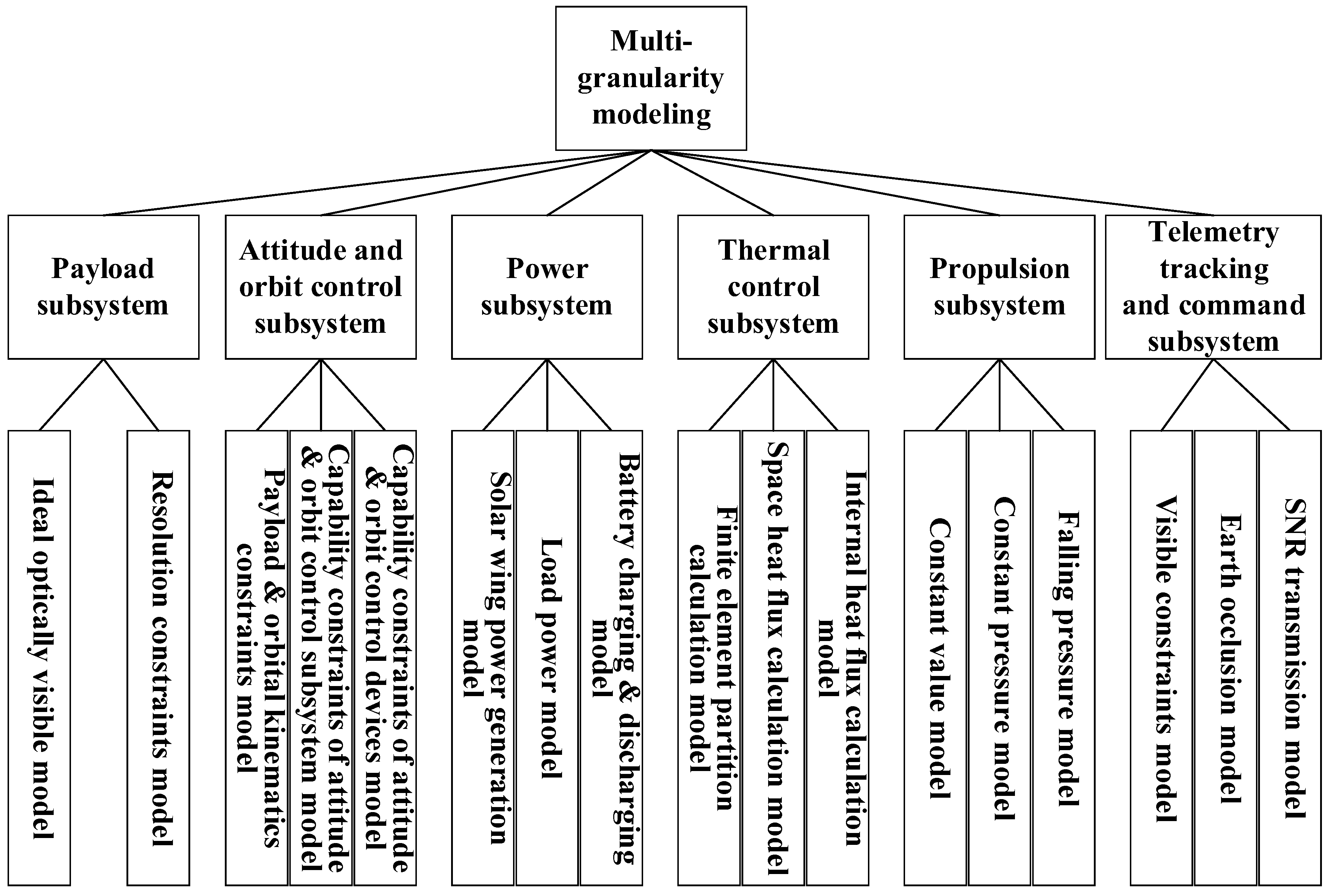
Satellite multi-granularity modeling can be divided into the payload subsystem, attitude and orbit control subsystem, power subsystem, thermal control subsystem, propulsion subsystem, telemetry tracking and command subsystem.The specific structure of multi-granularity modeling is shown in Figure 1.
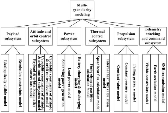
Figure 1.
The tree diagram of multi-granularity modeling.
2.2.1. Payload Subsystem
The payload subsystem model can be built with two granularities: ideal optical visible granularity and resolution-constrained granularity.
The former is characterized by the angle of visibility, which is determined by the target and the light shaft and can be calculated based on the location of the camera and the angle of connection between the two. If the angle is smaller than the corner of the field, it is considered to be optical visibility, otherwise, it is not visible. The latter granularity is constrained by the resolution of the payload and is determined by the smallest resolvable element in the image.
where is the angle of the target and the light shaft and is the visual angle.
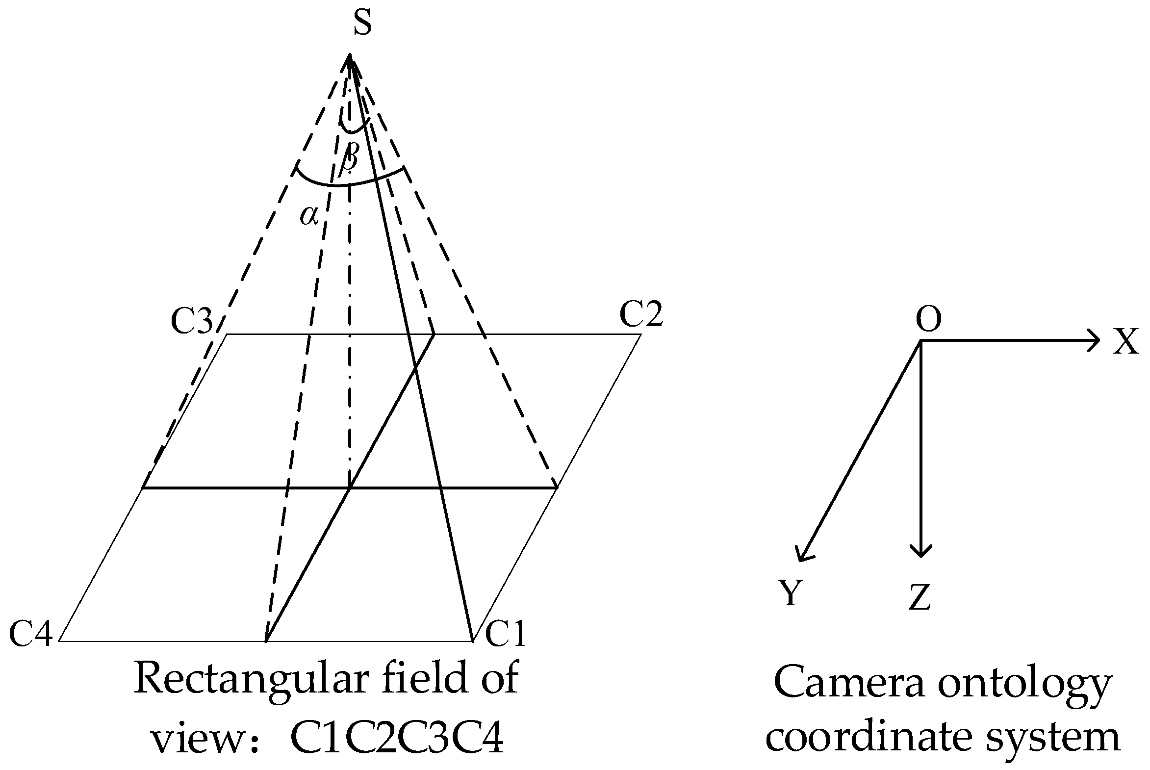
Resolution-constrained granularity needs to consider data generation, data compression, and data storage of the payload camera. The rectangular field of view generated by the optical camera is shown in Figure 2. S is a satellite camera, and C1C2C3C4 is the rectangular field of view.

Figure 2.
Optical area array camera rectangular viewing diagram.
Based on the camera’s field of view, the positions of the four points in a rectangle can be calculated. Images can be converted to pixel information and data after the fit resolution is selected. If the pixel data is empty, the amount of data generated is constant, otherwise, the amount of data generated is as follows,
where is the resolution of the rectangle image’s long side, is the resolution of the rectangle image’s short side, is image depth, is the data volume of the picture, the unit is the byte.
If the sampling frequency is , the total data volume generated in the period is
Data are stored by compression; compressibility is and the compressed data volume is
When data are transmitted to the Earth station, link transmission must be calculated. This calculation process is managed by the track telemetry and control subsystem and is shown in the telemetry and control subsystem.
2.2.2. Attitude and Orbit Control Subsystem
The attitude and orbit control subsystem model can be described as the payload and orbital kinematics constraints granularity, capability constraints of attitude and orbit control subsystem granularity, and capability constraints of attitude and orbit control devices granularity.
The payload and orbital kinematics constraints granularity is a mathematical representation that accounts for the changes in orbit and attitude kinematics parameters over time, without taking into consideration the control process. Orbit is calculated as an elliptical orbit, and the kinematics formula is
The first line in the formula represents the elliptical track motion equation, E is the eccentric anomaly, M is the mean anomaly, e is eccentricity, n is the average orbital angular velocity, and is perigee time.
Setting attitude mode as gaze mode, the expected attitude angle of the satellite can be calculated based on the projection of the target.
where , , and are roll angle, pitch angle, and yaw angle, where is the expected yaw angle.
Capability constraints of the attitude and orbit control subsystem granularity require the closed-loop control process of sensors, controllers, and actuators, as well as the consideration of the influence of force and torque on the attitude and orbit control state parameters.
Sensor model [32] is
where is measured value, is real value, is measured error. The measured error can be calculated using a normal distribution. is the theoretical model of the sensor, and is the error model of the sensor. is install information of sensor, is a celestial state, i.e., solar vector, Earth vector.
The output command of the satellite controller [32] is
where is a controller algorithm including an exclusion algorithm, filtering algorithm, attitude determination algorithm, and control algorithm. is the state parameters of the satellite controller, is the expected satellite state, and is related to the measurement parameters of the sensor and telecommand,
where is telecommand.
The expected satellite state includes default parameters for the controller and parameters set through ground telecommand, is a relation function,
where is the controller default parameters.
The real output value of the actuator [32] is as follows
where is the ideal output value of the actuator, and is the output error of the actuator. The output value of the actuator includes force, torque, and angular momentum. is the theoretical model of the actuator, and is the error model of the actuator. is install information of actuator.
For fixed actuators, the install parameter is invariable, only related to the initial install information .
For moving actuators, the install parameter is related to the initial state and motion parameter.
where is the install parameter of the moving actuator, is the motion parameter of the moving actuator, is the kinematics rule of the moving device, and is the initial install information of the moving device. The changes in motion parameters are related to the initial state, control commands, or telecommand
Moving devices of satellites include solar arrays, antenna, etc. For solar arrays, motion parameters mainly include the speed of the solar array and the rotation angle of the solar array . The install parameter mainly includes the normal vector of the solar array . For the antenna, the motion parameter mainly includes the rotation rate of the antenna , , and the rotation angle of the antenna , . The install parameter is the normal vector of the antenna .
The dynamic equation is as follows
where is environmental force, is control force. is environmental torque, is control torque, is the angular momentum of the satellite.
The capability constraints of attitude and orbit control devices granularity further considers the coupling effect between each device and the surrounding environment based on the previous granularity.
The error model of the sensor and actuator is
where and are coupling state variables of the sensor and actuator. There are mainly two types of state variables: one is transient state variables, which can be updated immediately after time, such as voltage and switch state. The other one is the steady-state state variable, which changes relatively slowly over time.
Taking a laser gyro as an example, considering the coupling with thermal field and radiation, the angular velocity measurement value is
where is the wavelength, is the normalized refractive index of the optical path, , are area and perimeter enclosed by a closed optical path, is a measurement of the frequency difference between the front and back beams of light,
where is the real value of frequency difference, is zero bias error, is random walk error, and is an error caused by the accumulation of radiation fluence. Temperature couples between and thermal field calculation, coupled with particle radiation. The error model is as follows
where , , are zero bias compensation coefficient obtained by fitting measurement data, is the temperature of a laser gyro, is lock zone threshold, is peak jitter rate, is laser gyro scale factor, is radiation flux along satellite orbit, is the relationship function between error and radiation flux.
Taking the wheel as an example, considering the coupling between friction coefficient and thermal field, the torque output by the wheel in the body coordinates is
where is output torque of the motor, is bearing static friction torque, is the frictional coefficient, is the speed of the wheel, and is the unit installation vector of the wheel. The output torque is as follows,
where is torque voltage ratio coefficient, is the input voltage.
Temperature coupling between and thermal field calculation. The model is as follows
where is the density of lube, is the amount of lube, is the specific heat of lube, is the difference between temperature and nominal temperature of the wheel, and is the bearing diameter of the wheel.
Taking into account the friction factor of bearings, the angular acceleration of the wheel is
where is the inertia of the wheel.
Device-level performance indicators must not only account for the impact of inter-subsystem interactions on device performance but also consider the varying degrees of impact that these interactions have on different parts of the device. For instance, the measurement accuracy of gyroscopes is affected by shaft temperature, with higher temperatures leading to greater errors. Therefore, it is important to consider the calculation of the bearing temperature field. However, the temperature of other parts of the satellite has a smaller impact, and therefore a multi-scale approach with local refinement and overall coarseness should be adopted when dividing the mesh.
2.2.3. Power Subsystem
The power subsystem is characterized by a set of parameters including the output of the solar array, load power consumption, battery charging and discharging, and remaining capacity. The calculation model of each parameter is as follows
(1) Output model of the solar array
The output model of a solar array can be modeled with constant output power granularity and considering solar array state granularity.
Constant power granularity refers to the fact that the solar array generates zero electricity in the shadow area and the output power is calculated at a constant value in the illumination area.
The considering solar array state granularity refers to the relationship between the output power of the solar array and the satellite’s state, taking into account the material characteristics of the solar array and the incidence angle of solar optics.
where is shadow area identification, is the power generated by sunlight, is an area of the solar array, is the power temperature coefficient of the solar array, is other parameter, is the normal vector of the solar array and included angle of solar vector, is difference between working temperature and standard temperature. is not only related to the position and attitude of the satellite but also to the relative angle of the sail relative to the body.
(2) Load power consumption
The load power can be built with three granularities: constant load granularity, considering device switch granularity, and considering device state granularity.
The power consumption in the constant load granularity is calculated using fixed values, which can be either the rated power or the average power consumption over a specified period.
The considering device switch granularity involves the real-time statistical analysis of the switch state of each device, as well as the power consumption of each device, which is constant and remains the same over time.
where is the total number of electrical devices, is the switch state of the device , power on is 1, power off is 0 and is the power of the device .
The considered device state granularity refers to the relationship between the actual power consumption and the device’s working state. For example, this includes the power consumption and speed of wheels. The formula is as follows
where is the inertia of the wheel, and is the angular velocity of the wheel, is the angular acceleration of the wheel.
(3) Battery charging and discharging
The battery charging and discharging model includes ideal battery granularity and nonideal battery granularity.
In the ideal battery granularity model, when the power generated by the solar array exceeds the electrical power of the equipment and the battery is not fully charged, the battery is charged at constant power, with any excess electricity dissipated through the charging regulator. Conversely, when the Earth shadow or power supply of the solar array is insufficient, the battery is discharged at constant power.
The consumption power of the charging regulator is as follows
where is the maximum charging power of the battery.
where is load power, is minimum battery capacity, and is maximum battery capacity.
Battery remaining capacity is as follows
where is the simulation step.
The power relationship in nonideal battery granularity is unaltered, but varying charging and discharging coefficients must be taken into account when calculating power consumption.
where is charging coefficients, is discharging coefficients.
2.2.4. Thermal Control Subsystem
The thermal balance expression of satellites in space is
where is the direct solar radiation heat absorbed by satellites, is the Earth infrared radiation heat absorbed by satellites, is the infrared radiation heat absorbed by the satellite, is space background heating amount, is the heat generated by the satellite, is a change in internal energy of satellites, is the heat emitted by satellites into space. Due to the low temperature of the spatial background and the small heating heat, the heating amount of the spatial background can be ignored.
The temperature field of the satellite is solved using the finite element method, and the thermal balance equation of each finite element node is [33]
where is node temperature, is node mass, is node specific heat capacity, is solar radiation heat, is Earth radiation heat, is Earth reflection radiation heat, is heat radiation, is heat conduction, is internal thermal power, is external surface heat dissipation, is internal surface heat dissipation, is node initial temperature.
The thermal control subsystem model includes three parts: finite element partitioning calculation, external heat flow calculation, and internal heat flow calculation.
(1) Finite element partition calculation model
The heat balance equation for each node remains constant regardless of the specific research object, but the number of nodes distributed throughout the satellite may vary depending on the research object. The thermal balance equations of each node remain unchanged, but the division of nodes in different parts of satellites can differ based on the research object. Taking Figure 3 as an example, the satellite structure mainly includes the main body, solar array, and various devices. When temperature is not the primary factor affecting certain indicators, the temperature of each part can be considered at a coarser level of detail. Typically, all structures and devices can be divided into meshes with the same level of accuracy. However, when calculating indicators that involve the temperature characteristics of a specific part, a finer mesh should be used for that part, while other parts can still use a coarser granularity to increase computational efficiency. All meshing is performed through Ansys software.
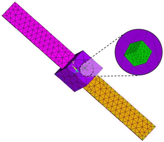
Figure 3.
Multi-scale division of finite element mesh.
(2) External heat flow calculation [33]
The external heat flow calculation model can be described as constant external heat flow granularity and node state external heat flow granularity.
The constant external heat flow granularity does not account for local temperature differences, and the radiation parameters are calculated using average values in the local film area and the light area, respectively.
The node state external heat flow granularity is a model that considers the orbit, attitude, and other states that need to be accounted for in the calculation of external heat flow, as well as material attributes.
Node solar radiation heat is
where is solar absorption rate on the outer surface of satellites, is solar constant, is the surface area of node , and is the direct solar radiation angle coefficient of the node .
where is the dot product of the vector and vector , is the shadow zone identification, is a solar vector, and is an illuminated surface normal vector.
Earth radiation heat of node is as follows
where is the outer surface emission rate of the node , is the average of surface infrared radiation density, and is the Earth’s infrared radiation angle coefficient of the node . Define , where is satellite orbital altitude, is the average radius of the Earth. When 0 ≤ ≤ , . When ≤ ≤ π, . When ≤ ≤
Earth reflection radiation heat of node is
where is the average reflection density of the Earth’s surface facing the solar radiation, and is the Earth’s infrared radiation factor of the node .
where is the Earth vector.
(3) Internal heat flow calculation [33]
The internal heat flow calculation model can be described as constant internal heat flow granularity and node state internal heat flow granularity.
The constant internal heat flow granularity is consistent with the constant external heat flow granularity, and all devices operate at their rated thermal power.
The node state internal heat flow granularity is consistent with node state external heat flow granularity.
Thermal radiation from other thermal nodes to node is
where is the absorption factor of node to node , is the emissivity of node , and is Boltzmann constant.
Other thermal nodes to the thermal conduction of node are
where is the conduction factor between node and node .
The internal thermal power of the node is equal to the sum of the thermal power of all devices in the node range
where is the total number of all devices belonging to the node , is the thermal power of the component
where is the work status of devices, The relationship function between and thermal power is .
External surface heat dissipation of node is
Internal surface heat dissipation of the node is as follows
where is the internal surface emissivity of the node .
2.2.5. Propulsion Subsystem
The model granularity of the propulsion subsystem includes constant granularity, constant pressure model granularity, and depressurization model granularity. The core state parameters include specific impulse and fuel consumption rates.
The relationship between the mass of the remaining propellant in the storage tank and time is
where is initial propellant mass in the tank, is mass consumption of propellant, is propellant consumption rate, is ignition command.
Constant granularity refers to the calculation of specific impulse and fuel consumption rates based on constant values.
The constant pressure model granularity is concerned with the relationship between specific impulse, fuel quality, and the working status of temperature, pressure, and valve switching duration.
where is flow coefficient, is the total area of the thruster injection hole, is the gravitational acceleration, and is the relative density of the propellant liquid.
The storage tank maintains constant gas pressure, that is . The gas mass in the tank can be obtained from the ideal gas equation.
where is the average molar mass of gas, and is the universal gas constant.
In the depressurization model granularity, the working status of the specific impulse, fuel quality consumption and temperature, pressure, and valve switch duration is related. The mass of gas in the storage tank is constant, that is . The gas pressure in the storage tank can be calculated through the ideal gas equation
2.2.6. TTC Subsystem
TTC subsystem includes communication visible constraint granularity, Earth occlusion granularity, and SNR transmission granularity.
The communication visible constraint granularity focuses on the connection state of the satellite and earth radar station and does not consider the specific transmission process.
The Earth occlusion granularity focuses on geometric constraints. When the satellite and the Earth station are not obstructed by the Earth, their transmission ability is considered connecting, otherwise disconnected. The elevation between the satellite and the Earth station can be calculated. The elevation angle is the angle formed by the horizon horizontal line where the ground station is located at the center line of the antenna. When the actual elevation angle is greater than the minimum elevation angle , it is determined that the two can communicate. Assuming that the position vector of satellites and Earth stations is and , the included angle and is .
Actual elevation
Transmission capacity is
In the SNR transmission granularity, the transmission capacity is influenced by factors such as the relative position of the receiver and transmitter, performance, data compression, and transmission loss, the basic transfer equation is as follows
where is the receiving antenna power, is the transmitter power, is the transmitter antenna gain, is receive antenna gain, is the path loss, is other various losses.
The unit of operating frequency f is MHz, and The distance d between two interfaces is measured in kilometers. mainly includes the influence of antenna pointing. Loss of transmitter antenna pointing is , the loss of receiver antenna pointing . The loss is related to the directional pattern of the antenna, A computational model for a point beam antenna is as follows
where is the angle between the Z-axis of the transmitting antenna instrument coordinate system and the vector between the transmitting node and the receiving node.
The current carrier-to-noise ratio from sender to receiver is
when , the sender from the receiver is normal, otherwise it will not be connected.
3. Selection of Effectiveness Evaluation Indicator Models for Remote Sensing Satellites
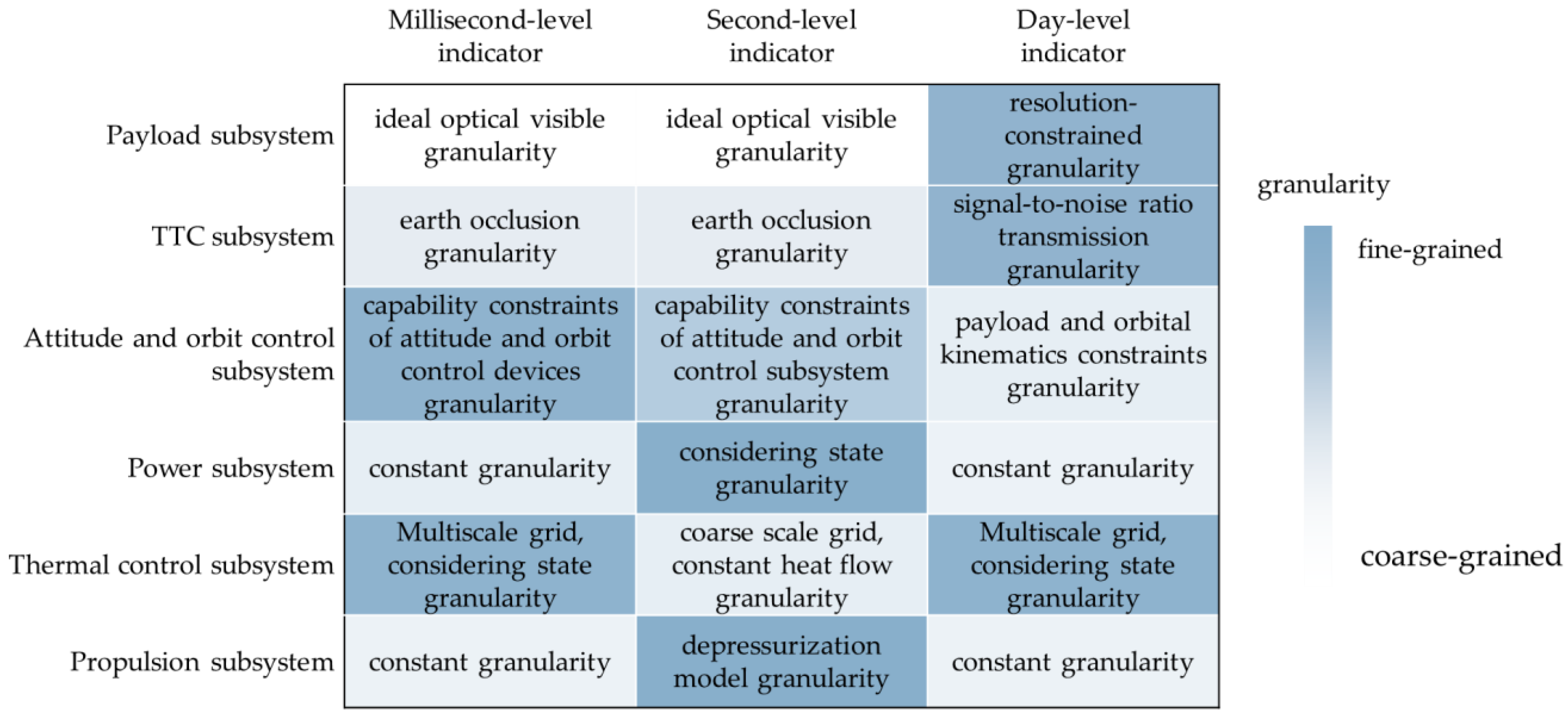
Capitalizing on the sparse nature of the satellite system, the effectiveness evaluation metrics are categorized into three groups based on time intervals: milliseconds, seconds, and days. As depicted in Figure 1, the satellite architecture consists of multiple subsystems, including payload, attitude and orbit control, power, thermal control, propulsion, and TTC. Each subsystem has various levels of granularity, as illustrated in Figure 4. When assessing each group of indicators, it is recommended to utilize the corresponding granularity level shown in Figure 4.
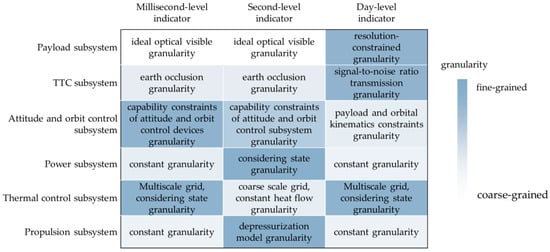
Figure 4.
Granularity combination recommended for effectiveness evaluation indicators calculation.
The millisecond-level indicator is primarily used to evaluate the performance of attitude control, requiring the use of finer simulation granularity for attitude sensors, controllers, and actuators. In contrast, other subsystems use coarser granularity. For instance, the payload subsystem selects the ideal optical visible granularity, while the TTC subsystem selects the Earth occlusion granularity. The attitude and orbit control subsystem selects the capacity constraints of attitude and orbit control devices granularity. The power subsystem selects the constant granularity. As for the thermal control subsystem, the device mesh should be finely divided, while the structures such as the body and solar array should be coarser. The external and internal heat flows should be calculated using node state granularity. The propulsion subsystem selects constant granularity. When establishing simulation condition, it is recognized that the overall temperature change cycle is influenced by the annual cycle, which is much greater than the time required for millisecond-level simulations. Consequently, the two stages of local shadow and light are based on the two seasons of winter and summer, with simulation time spans of several thousands of seconds and step intervals of 0.1 s.
The second-level indicator is primarily used to evaluate the performance of power and propulsion. The power subsystem selects the considering state granularity, while the propulsion subsystem selects the depressurization mode granularity. Other subsystems use coarser granularity, such as the payload subsystem selecting the ideal optical visible granularity, the TTC subsystem selecting the Earth occlusion granularity, and the attitude and orbit control subsystem selecting the capability constraints of attitude and orbit control subsystem granularity. The mesh of the thermal control subsystem can be broadly classified into two categories, and internal and external heat flows are computed using constant values. To collect simulation statistics, the light area and the shadow area are selected. The integration duration for each stage is set at several thousands of seconds, with a step size of 1 s.
The day-level indicator is mainly used to evaluate load observation, TTC performance, and thermal control performance. The payload subsystem selects the resolution-constrained granularity, the TTC subsystem selects the SNR transmission granularity. For the thermal control subsystem, the devices and solar array are finely divided, while the body is coarser. The calculation of internal and external heat flow selects node states granularity. The granularity of other subsystems is relatively coarse. The attitude and orbit control subsystem selects the payload and orbital kinematics constraints granularity, the power subsystem and the propulsion subsystem select the constant granularity. When setting up the working conditions, the integration duration for each stage is about one year, and the integration step is 100 s.
When calculating indicators, the granularity selected by each model is not fixed, but selected according to a certain probability. Figure 4 shows the maximum possible recommended particle size. Given the unique characteristics of individual satellites, a tailored approach is necessary to identify the most suitable combination of indicators and model granularities. By implementing a multi-granularity model, iterative evaluation processes can be employed to refine simulation granularity at each iteration. In practical engineering applications, fine-tuned adjustments can be made based on evaluation results to achieve an optimal balance between computing accuracy and resource utilization. This approach enables the optimization of indicator grouping and model granularities for efficient performance assessment.
4. Simulation Case
4.1. Millisecond-Level Time Resolution Indicator Calculation
The orbital elements are as follows: the semi-major axis is 6,994,596.133 m, the eccentricity is 0.0001537, the inclination is 97.8416°, the right ascension of ascending node is 155.985°, the argument of perigee is 92.481°, and the true anomaly is 0°.
The millisecond-level indicators mainly include the attitude and orbit control subsystem. A comparison between the coupled model and the uncoupled model of attitude orbit control subsystem should be studied. The attitude angles of the attitude and orbit control subsystem without considering thermal coupling, considering the coarse mesh and considering the multi-scale mesh, are compared, as shown in Figure 5. When the coupling effect is not considered, the noise model of the device is a normal distribution model and the attitude angle changes randomly around a constant value. Considering the influence of temperature on attitude and orbit control devices, when the mesh is divided roughly, the device temperature changes with the temperature of the whole satellite over a long period. When the mesh is divided into different scales and the local temperature is considered, the components are more affected by the local temperature, and the temperature changes quickly there. The impact on the attitude control effect is also faster.
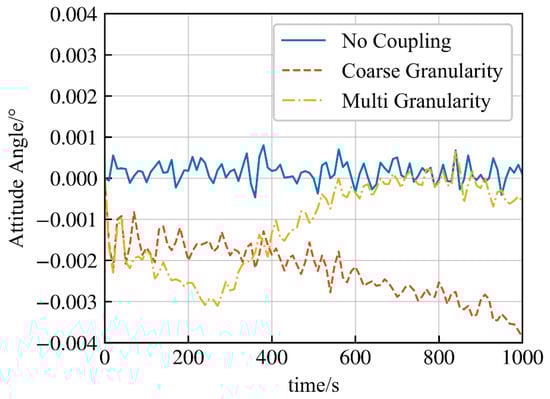
Figure 5.
Comparison diagram of attitude angle measurement for different models.
The calculation of indicators is verified under different granularity models and different working conditions. The models are the coarse granularity model, the multi-granularity model, and the finest granularity model. The coarsest granularity model of attitude and orbit control subsystem considers the device level, but the mesh is divided coarsely, which only reflects the temperature change of the whole satellite and cannot reflect the temperature of local devices. The multi-granularity model considers the characteristics of the devices, including the influence of local temperature on the noise. The mesh of the temperature of the device is finer, and the body and solar array are rough. The finest granularity model considers the characteristics of devices, and the mesh division of devices, body, and sailboard is very fine.
The working states are statistically analyzed in four time periods: UTC 12:40:50 on 21 June 2022 (Summer Shadow Zone), 13:50:50 on 21 June 2022 (Summer Light Zone), 13:29:40 on 21 June 2022 (Winter Shadow Zone), and 14:25:50 on 21 December 2022 (Summer Light Zone). The simulation step is 0.1 s and the total simulation time is 1600 s.
The results are shown in Table 1.

Table 1.
Comparison of millisecond-level time resolution indicators.
According to the indicator calculation results, it can be seen that the attitude measurement accuracy, attitude pointing accuracy, and attitude stable accuracy of the shadow area are generally lower than those of the light area. This is because the working temperature of the lighting area devices is close to the nominal temperature of 20 °C, while the ground shadow area temperature is around −20~−40 °C, far deviating from the nominal temperature. Therefore, the measurement error of the sensor is greater than that of the lighting area. The calculation results of the finest granularity model and the multi-granularity model are close. Comparing the simulation time of the three types of models, the coarse granularity model takes 93 s, the multi-granularity model takes 262 s, and the fine granularity model takes 1132 s. The calculation time of the multi-granularity model is much shorter than that of the finest granularity model, but the calculation accuracy is the same.
4.2. Second-Level Time Resolution Indicator Calculation
The orbit parameter selections are the same as above.
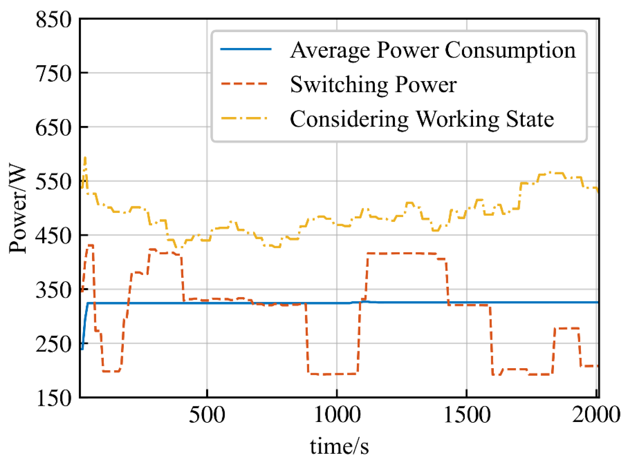
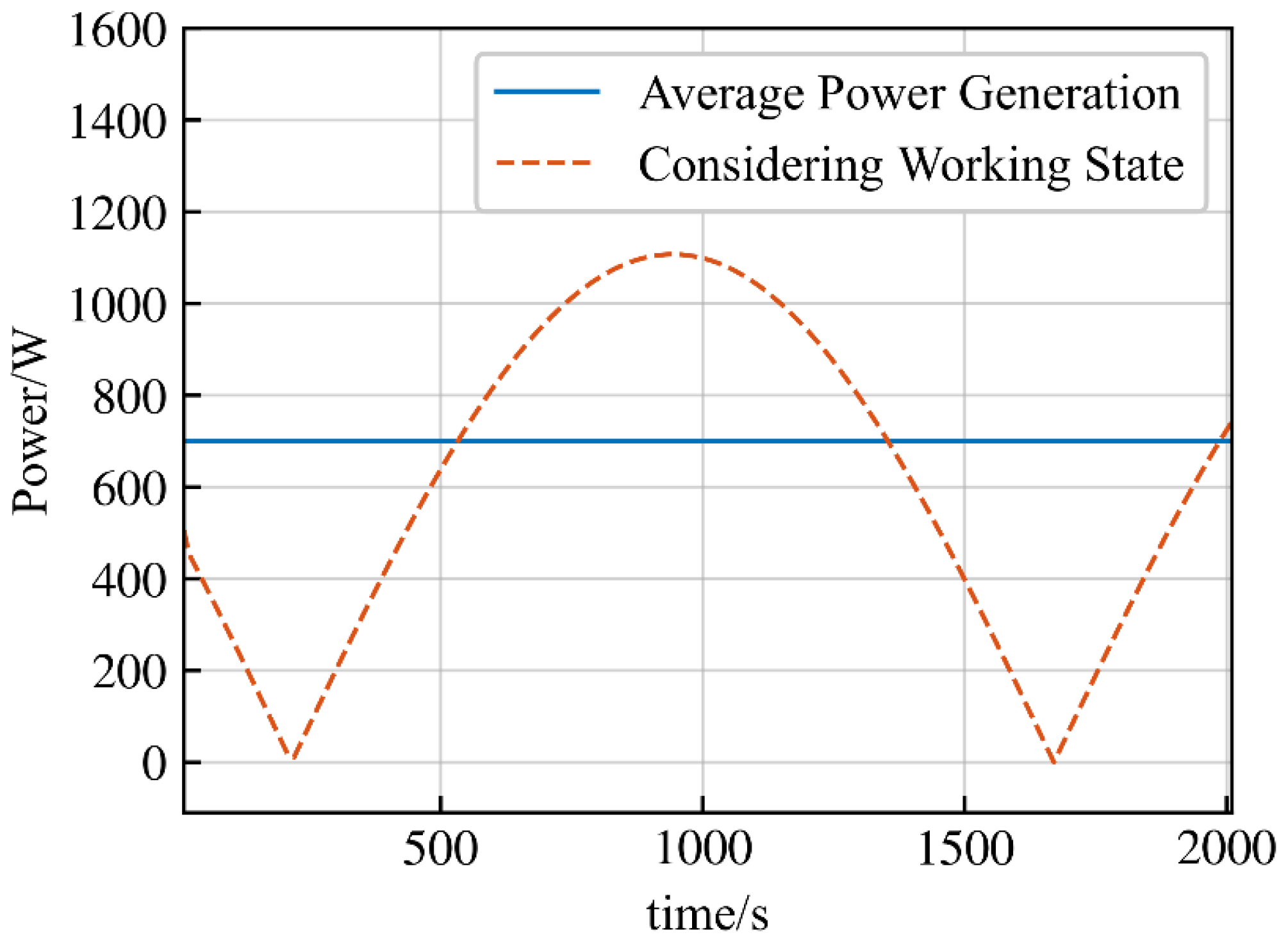
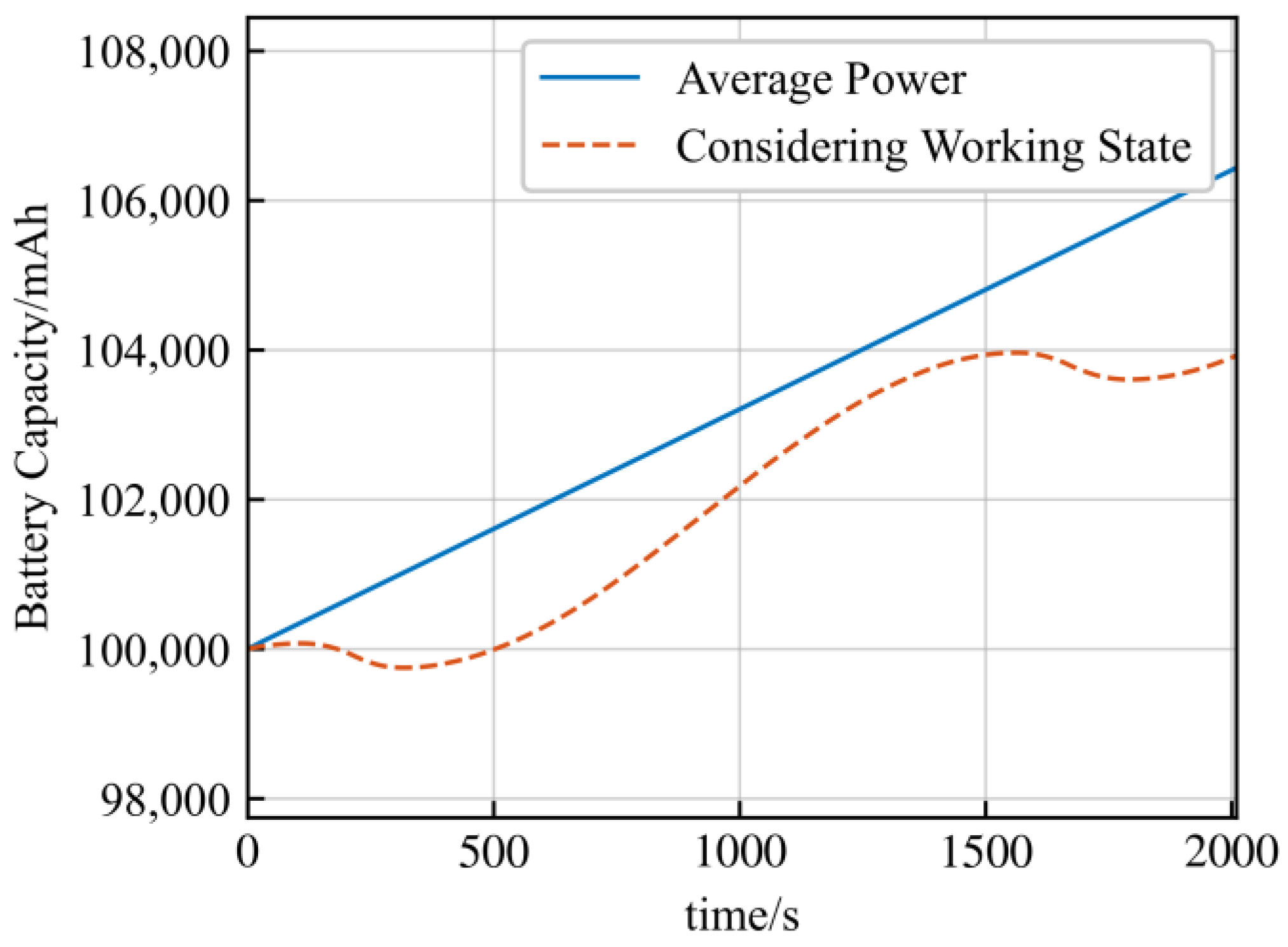
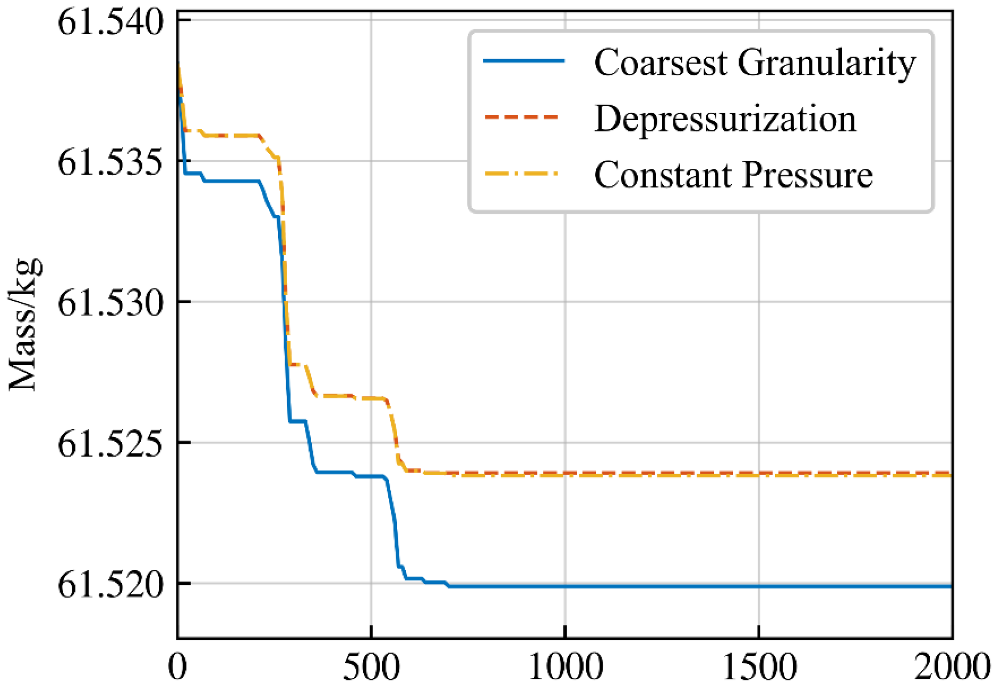
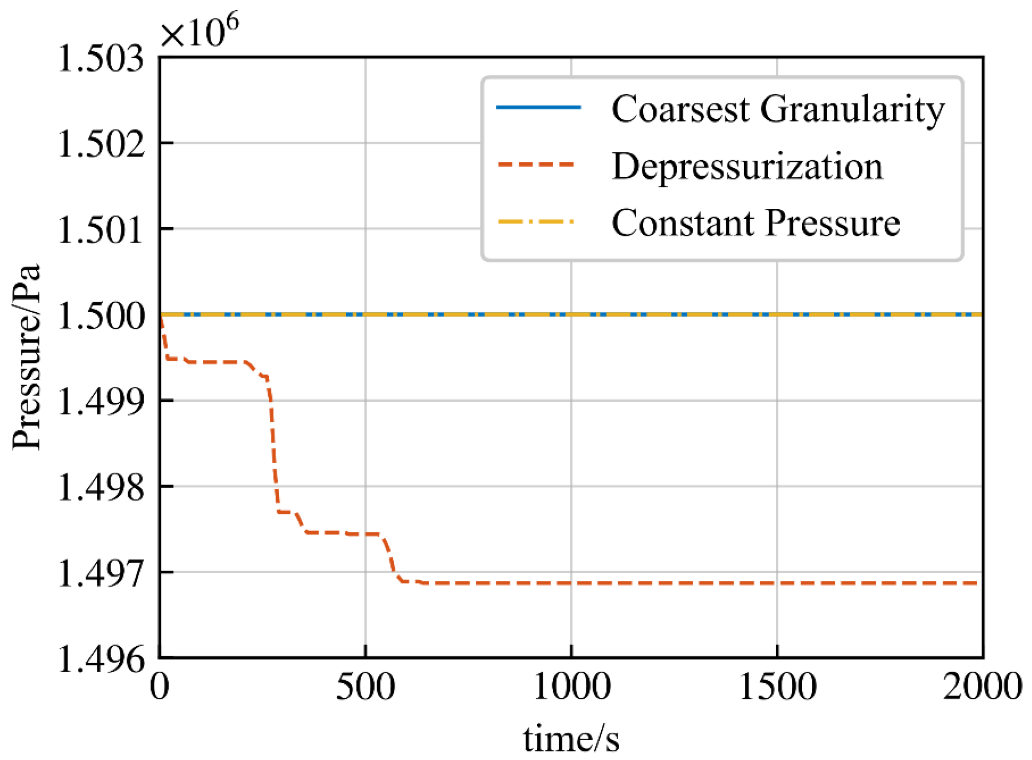
The second-level indicators mainly include the power subsystem and propulsion subsystem. A comparison between the coupled model and uncoupled model should be studied. The parameters of the power subsystem and propulsion subsystem are compared in the following figures (Figure 6, Figure 7, Figure 8, Figure 9 and Figure 10). As shown in the figures, comparing the state variables of the power subsystem under the granularity of the constant granularity, considering device switch granularity, and considering device state granularity, when only the average power generation, power consumption, and power storage are considered, the state is a straight line, and the switching granularity is considered to be stepped. Neither of these two models can fully reflect the real state change, but considering device state granularity can better reflect the coupling change between the working state of the device and the electric quantity. The propulsion subsystem models of constant value granularity, constant pressure mode granularity, and depressurization mode granularity also reflect the above rules.
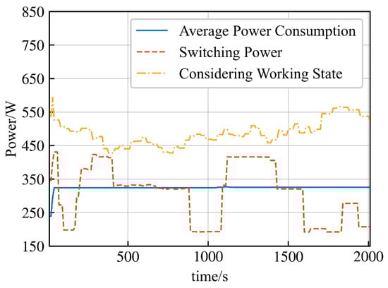
Figure 6.
Load power comparison diagram.
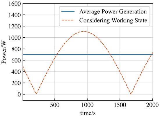
Figure 7.
Comparison diagram of solar array output power.
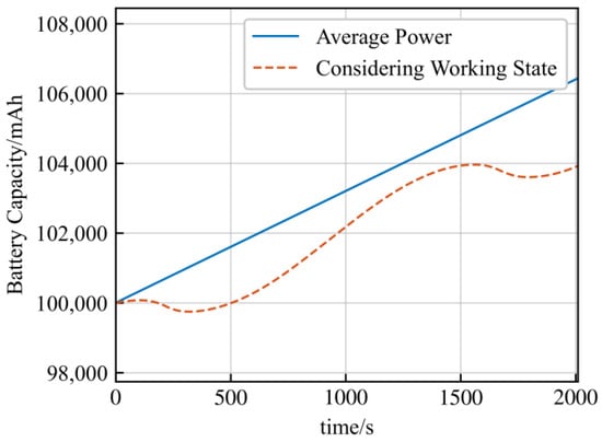
Figure 8.
Comparison diagram of remaining battery power.
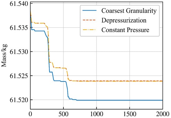
Figure 9.
Comparison diagram of fuel mass.
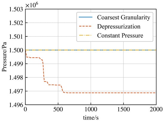
Figure 10.
Comparison diagram of Helium pressure in the fuel tank.
Comparing the indicator calculations of the three models for the power subsystem and the propulsion subsystem, they are the coarse granularity model, the multi-granularity model, and the finest granularity model. The attitude and orbit control subsystem of the coarse granularity model is the subsystem capability constraint granularity, the power and propulsion are constant granularity, and the mesh division is coarse. The attitude and orbit control subsystem of the multi-granularity model is the capability constraints of attitude and orbit control subsystem granularity, the power subsystem is the granularity of considering the state changes of the devices, and the propulsion subsystem is the depressurization mode, and the mesh is divided into multiple granularities according to different parts. The finest granularity model: the attitude and orbit control subsystem is the capability constraint of the attitude and orbit control devices granularity, the power subsystem is the granularity of considering device state changes and the propulsion subsystem is depressurization mode granularity. The mesh division is relatively fine.
The working state was configured at UTC 12:40:50 on 21 June 2022. The simulation step was 1 s and the total simulation time was 2000 s. The results are shown in Table 2.
Table 2.
Second-level indicator statistics.
The simulation time of the three types of models is 154 s for the coarse granularity model, 469 s for the multi-granularity model, and 2018 s for the finest granularity model. The calculation time of the multi-granularity model is much shorter than that of the finest granularity model, but the calculation accuracy is the same.
4.3. Day-Level Time Resolution Indicator Calculation
The orbit parameter selections are the same as above.
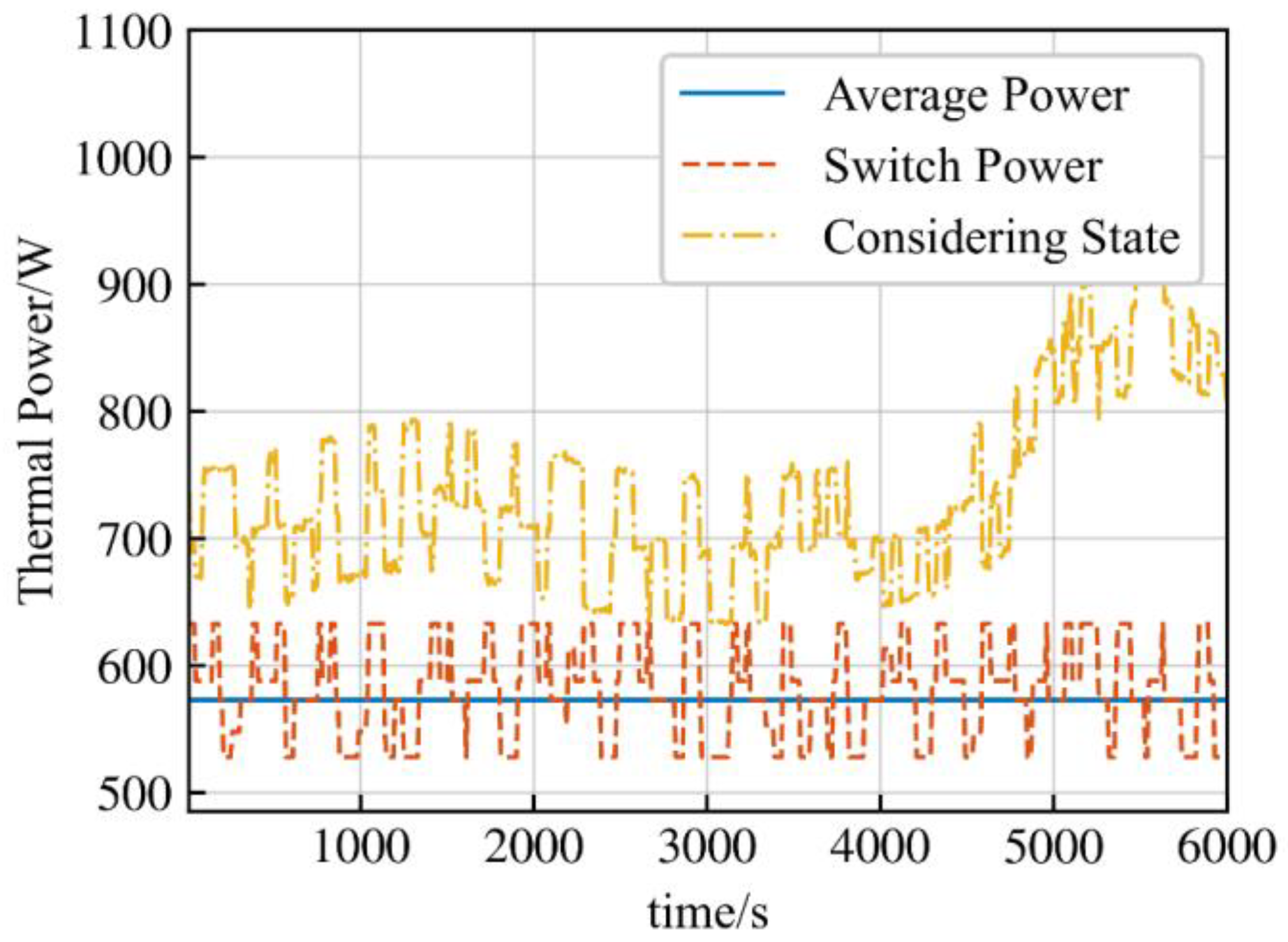
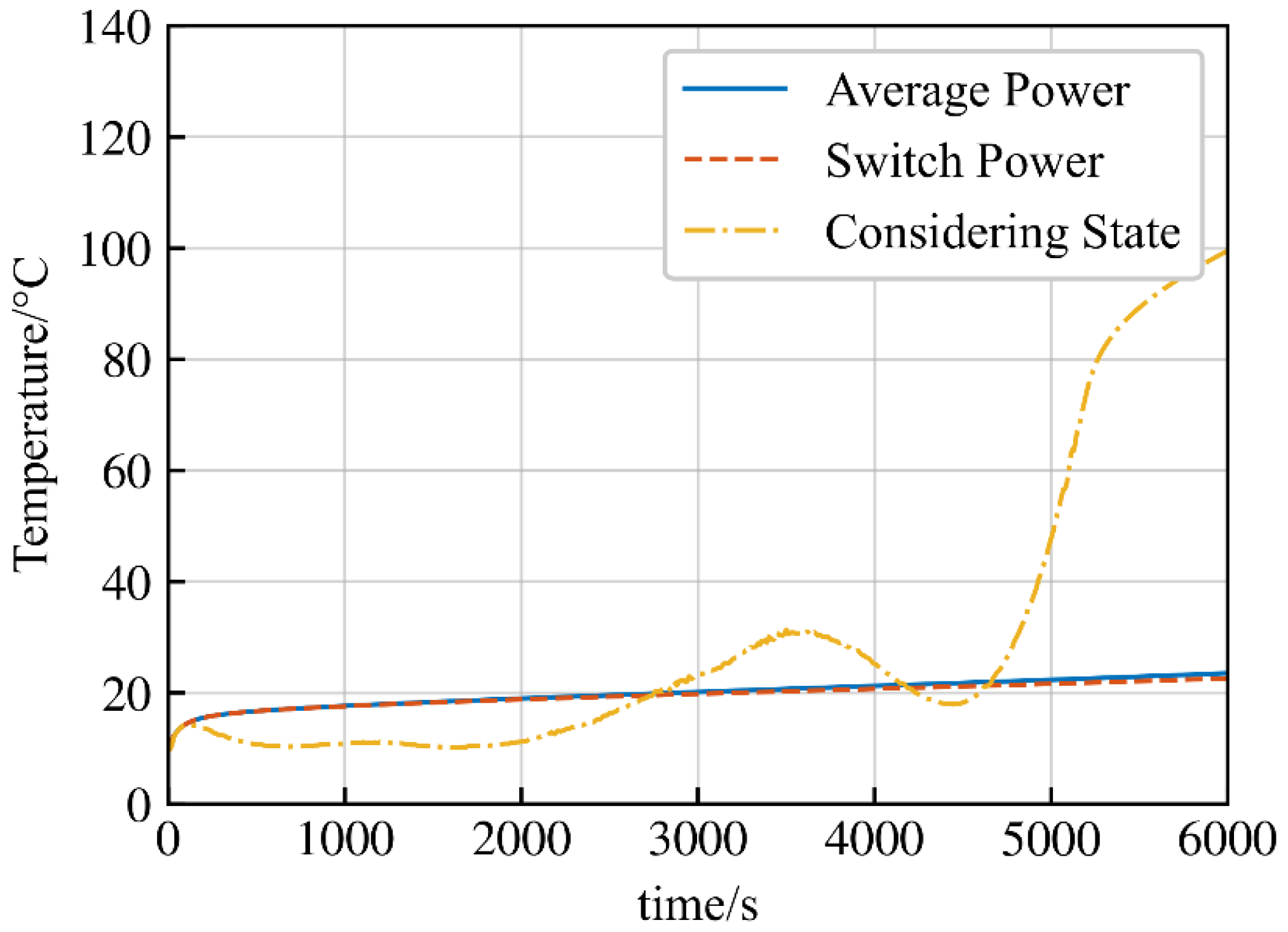
The day-level indicators mainly include the thermal control subsystem and TTC subsystem. A comparison between coupled model and uncoupled model should be studied. The parameters of the thermal control and TTC subsystem are compared in the following figures (Figure 11, Figure 12, Figure 13, Figure 14 and Figure 15). Comparing the state variables of the thermal control subsystem under the constant granularity, considering device switching granularity and considering the device state granularity, it can be seen that the change law is similar to that of the power subsystem in Figure 11 and Figure 12.

Figure 11.
Comparison diagram of thermal power of devices.
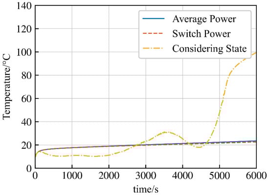
Figure 12.
Comparison diagram of momentum wheel temperature.
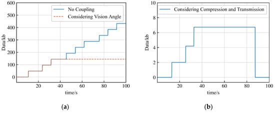
Figure 13.
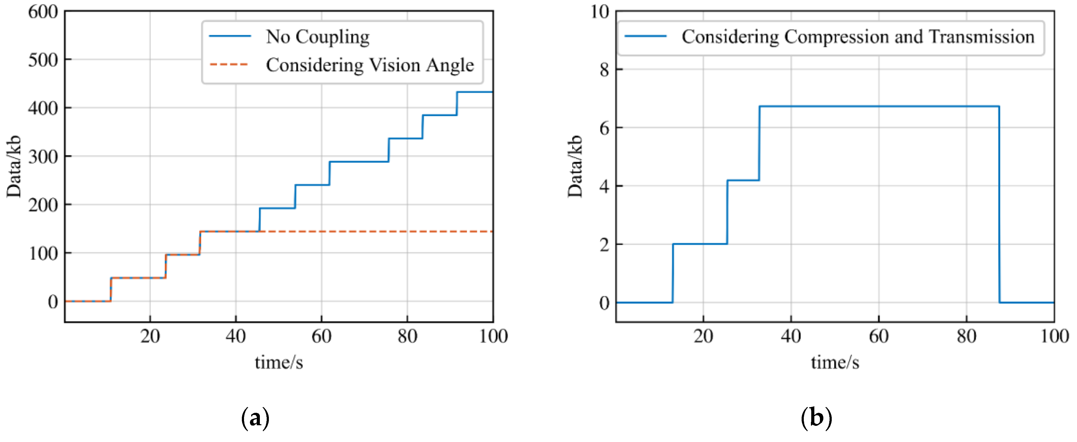
Changes in data stored in different models. (a) Uncoupled model and optical visible model. (b) Considering data compression and transmission models.
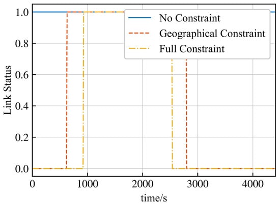
Figure 14.
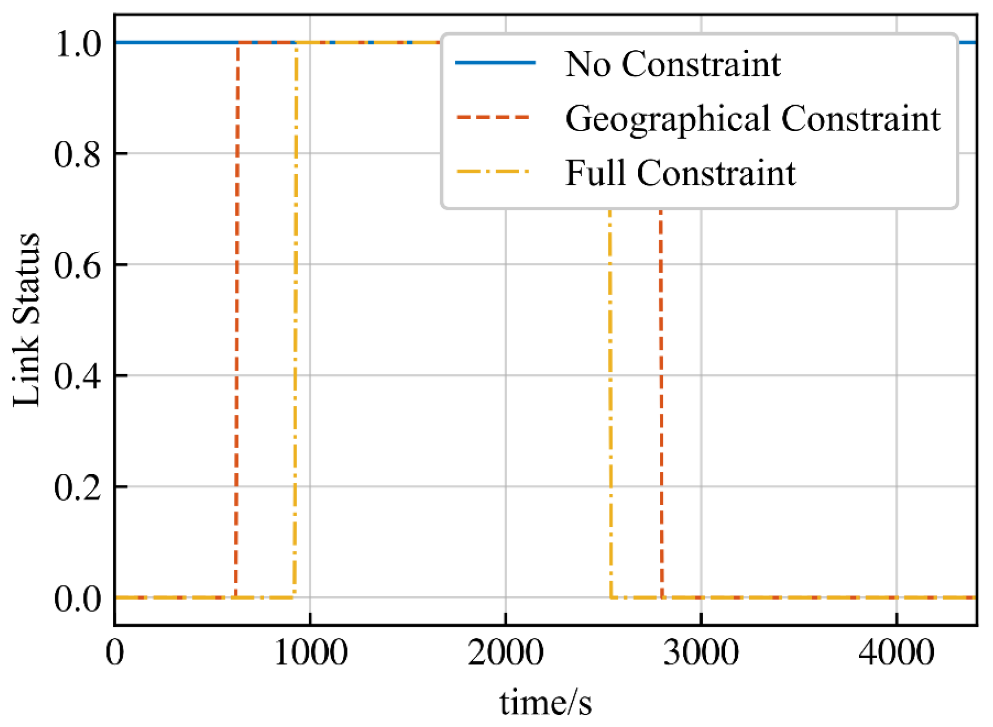
Comparison diagram of link state changes in different models.
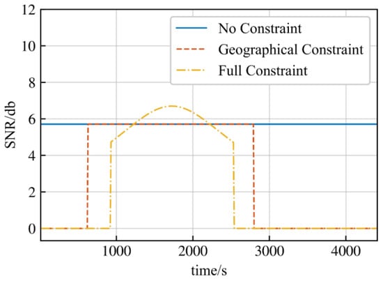
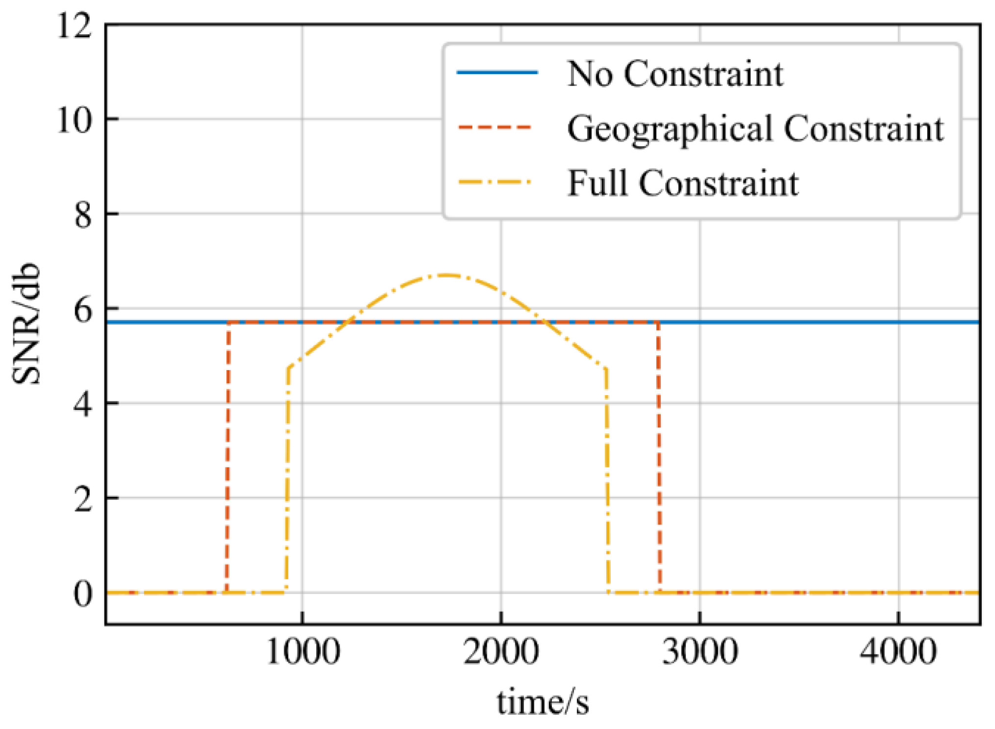
Figure 15.
Comparison diagram of SNR changes of different models.
Comparing the indicator calculation results of the three models, the coarse granularity model, multi-granularity model, and the finest granularity model, the difference between the models is that the mesh division of the coarse granularity model is rough, the attitude and orbit control subsystem uses payload and orbital kinematics constraints granularity. The mesh of the multi-granularity model is divided according to the size requirements of devices and structures, the attitude and orbit control subsystem in the multi-granularity model uses the payload and orbital kinematics constraints model. All meshes in the finest granularity model is very fine, and other systems such as attitude and orbit control subsystem are the finest granularity.
The working state was configured at UTC 12:40:50 on 21 June 2022. The simulation step was 100 s and the total simulation time was 1 year. The results are shown in Table 3.
Table 3.
Day-level indicator statistics.
As shown in the table, as the life of the satellite decreases, the heat generated by the devices increases, increasing the temperature indicators of the satellite. The simulation time of the three types of models is 2986 s for the coarse granularity model and 5823 s for the multi-granularity model. The simulation time of the finest granularity model is slower than the real-time, and it is unrealistic to use this model for calculation.
In Figure 13, optical payload and the TTC models of different granularity are compared. The uncoupled optical model can always take pictures of the target, and the data stored on the satellite continues to increase. Considering the visible granularity of the target is to take pictures when the target is within the field of view of the optical axis, and not to take pictures for the rest of the time. The finest granularity not only considers whether the target is visible, but also pictures can be compressed and downloaded to the ground, so the amount of data stored in it is much smaller than the previous two and can be cleared.
As shown in Figure 14 and Figure 15, the finer the granularity of the TTC models, the more constraints they are subject to, and the more stringent the conditions for communication with ground stations. When there is no constraint, the satellite, and the ground station can communicate all the time, and the SNR is constant. When considering the Earth occlusion granularity, only when the communication link between the two is not occluded by the Earth can they have communication capability, and the SNR is also constant. In the full constrain state, the SNR varies with the path conditions such as the distance between the satellite and the ground station. When it is less than a certain threshold, even if the two are on the same side of the Earth, they may not be connected.
Different models of payload and TTC indicators are calculated as follows. The ideal visibility model is that the optical payload is always visible to the target, and the satellite communicates with the ground station in real-time. Both the optical load and the communication occlusion of the Earth occlusion model consider the occlusion effect of the Earth. The finest model is the optical load considering compressibility and transmission, and the TTC subsystem considering the SNR ratio transmission granularity. The results are shown in Table 4.
Table 4.
Payload and communication link indicator statistics.
It can be seen from the table that as the granularity of the model becomes finer and more constraints are considered, the probability of target discovery will decrease, and the longer the target response time is, the lower the measurement and control coverage rate will be.
5. Conclusions
Reasonable and scientific performance evaluation provides a powerful reference for the demonstration and development of remote sensing satellite systems. Aiming at the problem of coupling multi-dynamic and multi-spatial scales in a satellite digital twin model in the effectiveness evaluation of remote sensing satellites, this paper proposes a method to calculate the effectiveness indicators by using multi-granularity modeling. The multi-granularity model in this paper takes into account the coupling effects of device states and attitude and orbit control, power, thermal control, and other subsystems. From the simulation results, it can be seen that the change in parameters of the uncoupled model has nothing to do with its own working state over time, and the component running states have no effect on the change in model parameters, while the trend of the parameters of the coupled model over time is closer to reality. For the millisecond-level, second-level, and day-level indicators, the simulation results of the multi-granularity model evaluation indicators compared with the single-granularity evaluation indicators show that the calculation accuracy of the multi-granularity model indicators is much higher than that of the coarse-grained model, and is close to the accuracy of the most fine-grained model. Multi-grained models run much faster than fine-grained models, but slower than coarse-grained models. In particular, for the simulation of the thermal control model, even the simulation time of the fine-grained model is slower than the real time, which loses the meaning of simulation. Compared with the single-granularity model, the accuracy of the evaluation results of the multi-granularity model meets the requirements and the calculation efficiency is higher, which verifies the feasibility and effectiveness of the multi-granularity model.
In order to strengthen the evaluation of multi-granularity modeling and its applicability, looking toward to the future, research can be carried out from two aspects. According to the missions of different satellites, multi-granularity models of different types of satellites will be constructed to complete the performance evaluation. For high real-time evaluation requirements, the machine learning evaluation model will be trained using the simulation data of the multi-granularity model to achieve rapid evaluation.
Author Contributions
Conceptualization, Y.D. and M.L.; methodology, M.L.; software, M.L.; validation, M.L.; formal analysis, M.L.; investigation, M.L.; resources, M.L.; data curation, M.L.; writing—original draft preparation, M.L.; writing—review and editing, M.L.; visualization, M.L.; supervision, Y.D.; project administration, M.L.; funding acquisition, Y.D. All authors have read and agreed to the published version of the manuscript.
Funding
This research received no external funding.
Data Availability Statement
Not applicable.
Acknowledgments
This work was partially supported by the Key Laboratory of Spacecraft Design Optimization and Dynamic Simulation Technologies, Ministry of Education.
Conflicts of Interest
The authors declare no conflict of interest.
References
- Weiss, M.; Jacob, F.; Duveiller, G. Remote Sensing for Agricultural Applications: A Meta-Review. Remote Sens. Environ. 2020, 236, 111402. [Google Scholar] [CrossRef]
- Farhadi, H.; Mokhtarzade, M.; Ebadi, H.; Beirami, B.A. Rapid and Automatic Burned Area Detection Using Sentinel-2 Time-Series Images in Google Earth Engine Cloud Platform: A Case Study over the Andika and Behbahan Regions, Iran. Environ. Monit. Assess. 2022, 194, 369. [Google Scholar] [CrossRef]
- Wang, Y.; Zhang, Y.; Chen, Y.; Wang, J.; Bai, H.; Wu, B.; Li, W.; Li, S.; Zheng, T. The Assessment of More Suitable Image Spatial Resolutions for Offshore Aquaculture Areas Automatic Monitoring Based on Coupled NDWI and Mask R-CNN. Remote Sens. 2022, 14, 3079. [Google Scholar] [CrossRef]
- Dhanaraj, K.; Angadi, D.P. Land Use Land Cover Mapping and Monitoring Urban Growth Using Remote Sensing and GIS Techniques in Mangaluru, India. GeoJournal 2022, 87, 1133–1159. [Google Scholar] [CrossRef]
- Farhadi, H.; Esmaeily, A.; Najafzadeh, M. Flood Monitoring by Integration of Remote Sensing Technique and Multi-Criteria Decision Making Method. Comput. Geosci. 2022, 160, 105045. [Google Scholar] [CrossRef]
- Chen, Y.; Tao, F. Potential of Remote Sensing Data-Crop Model Assimilation and Seasonal Weather Forecasts for Early-Season Crop Yield Forecasting over a Large Area. Field Crops Res. 2022, 276, 108398. [Google Scholar] [CrossRef]
- Cui, Z.; Li, Q.; Cao, Z.; Liu, N. Dense Attention Pyramid Networks for Multi-Scale Ship Detection in SAR Images. IEEE Trans. Geosci. Remote Sens. 2019, 57, 8983–8997. [Google Scholar] [CrossRef]
- Wang, J.; Song, G.; Liang, Z.; Demeulemeester, E.; Hu, X.; Liu, J. Unrelated Parallel Machine Scheduling with Multiple Time Windows: An Application to Earth Observation Satellite Scheduling. Comput. Oper. Res. 2023, 149, 106010. [Google Scholar] [CrossRef]
- Peng, G. Index System Construction of Information Support Capability Evaluation of Remote Sensing Satellite Task-Oriented. Command Control Simul. 2019, 41, 5–19. [Google Scholar] [CrossRef]
- Liu, F.; Li, L.; Meng, X. Research on Construction Model of the Capacity Index System for Remote Sensing Satellite System. Spacecr. Recovery Remote Sens. 2017, 38, 40. [Google Scholar] [CrossRef]
- Zhigeng, F.; Shuang, W.; Xiaoli, Z.; Yunke, S. ADC-GERT Network Parameter Estimation Model for Mission Effectiveness of Joint Operation System. J. Syst. Eng. Electron. 2021, 32, 1394–1406. [Google Scholar] [CrossRef]
- Liu, X.; Yang, X.; Zhang, T.; Wang, Z.; Zhang, J.; Liu, Y.; Liu, B. Remote Sensing Based Conservation Effectiveness Evaluation of Mangrove Reserves in China. Remote Sens. 2022, 14, 1386. [Google Scholar] [CrossRef]
- Li, H.; Li, D.; Li, Y. A Multi-Index Assessment Method for Evaluating Coverage Effectiveness of Remote Sensing Satellite. Chin. J. Aeronaut. 2018, 31, 2023–2033. [Google Scholar] [CrossRef]
- Zheng, Z.; Li, Q.; Fu, K. Evaluation Model of Remote Sensing Satellites Cooperative Observation Capability. Remote Sens. 2021, 13, 1717. [Google Scholar] [CrossRef]
- Li, J.; Dong, Y.; Xu, M.; Li, H. Genetic Programming Method for Satellite System Topology and Parameter Optimization. Int. J. Aerosp. Eng. 2020, 2020, 6673848. [Google Scholar] [CrossRef]
- Shen, Q.; Yue, C.; Goh, C.H.; Wang, D. Active Fault-Tolerant Control System Design for Spacecraft Attitude Maneuvers with Actuator Saturation and Faults. IEEE Trans. Ind. Electron. 2019, 66, 3763–3772. [Google Scholar] [CrossRef]
- Wu, X.; Dong, Y. Hierarchical Model Updating Method for Vector Electric-Propulsion Satellites. Appl. Sci. 2023, 13, 4980. [Google Scholar] [CrossRef]
- Zammit, S.; Zammit, S. Control and Dynamics Simulation Facility at Hughes Space and Communications. In Proceedings of the Modeling and Simulation Technologies Conference; American Institute of Aeronautics and Astronautics, New Orleans, LA, USA, 11 August 1997. [Google Scholar]
- Schaaf, J.C.; Thompson, F.L. System concept development with virtual protlotyping. In Proceedings of the 1997 Winter Simulation Conference, Atlanta, GA, USA, 7–10 December 1997. [Google Scholar]
- Grieves, M.W. Product Lifecycle Management: The New Paradigm for Enterprises. IJPD 2005, 2, 71. [Google Scholar] [CrossRef]
- Martínez-Olvera, C. Towards the Development of a Digital Twin for a Sustainable Mass Customization 4.0 Environment: A Literature Review of Relevant Concepts. Automation 2022, 3, 197–222. [Google Scholar] [CrossRef]
- Li, J.; Dong, Y. Multi-Granularity Genetic Programming Optimization Method for Satellite System Topology and Parameter. IEEE Access 2021, 9, 89958–89971. [Google Scholar] [CrossRef]
- Wang, X.; Li, D.; Zhang, Y. Satellite Design; China Astronautic Publishing House: Beijing, China, 2014; ISBN 978-7-5159-0827-4. [Google Scholar]
- Qu, D.; Lu, Y.; Tao, Y.; Wang, M.; Zhao, X.; Lei, X. Study of Laser Gyro Temperature Compensation Technique on LINS. In Proceedings of the 2019 26th Saint Petersburg International Conference on Integrated Navigation Systems (ICINS), St. Petersburg, Russia, 27–29 May 2019; IEEE: Saint Petersburg, Russia; pp. 1–6. [Google Scholar]
- Huang, H.-Z.; Yu, K.; Huang, T.; Li, H.; Qian, H.-M. Reliability Estimation for Momentum Wheel Bearings Considering Frictional Heat. Eksploat. I Niezawodn. Maint. Reliab. 2020, 22, 6–14. [Google Scholar] [CrossRef]
- Dong, Y.; Li, Z.; Lei, M. Research on Concept of Digital Satellite. Aerosp. Shanghai 2021, 38, 1–12. [Google Scholar] [CrossRef]
- Tang, Z.; Xu, Y.; Jiang, B.; Liao, H.; Zhao, Y. Integrated Structure and Precision Control of Flat Voice Coil Actuator for Non-contact Satellite. J. Eng. 2019, 2019, 566–570. [Google Scholar] [CrossRef]
- Zhong, X.; He, Y.; Liu, Q.; Wei, X. Power Control Approach in Distributed Satellite Cluster Network Based on Presetting and Prediction. In Proceedings of the 2016 IEEE Information Technology, Networking, Electronic and Automation Control Conference, Chongqing, China, 20–22 May 2016; IEEE: Chongqing, China; pp. 265–269. [Google Scholar]
- Feng, T.; Chen, X.; Zhang, J.; Guo, J. Passive Satellite Solar Panel Thermal Control with Long-Wave Cut-Off Filter-Coated Solar Cells. Aerospace 2023, 10, 108. [Google Scholar] [CrossRef]
- Li, Z.; Dong, Y.; Li, P.; Li, H.; Liew, Y. A Real-Time Effectiveness Evaluation Method for Remote Sensing Satellite Clusters on Moving Targets. Sensors 2022, 22, 2993. [Google Scholar] [CrossRef] [PubMed]
- Zhao, Y. Study on the Theory and Application of Multidisciplinary Design Optimization for the Satellite System; Graduate School of National University of Defense Technology: Changsha, China, 2006. [Google Scholar]
- Dong, Y.; Chen, S.; Su, J.; Hu, D. Dynamic Simulation Technology of Satellite Attitude Control; Science Press: Beijing, China, 2010; ISBN 978-7-03-028248-4. [Google Scholar]
- Li, Z. Satellite Thermal Control Technology; China Astronautic Publishing House: Beijing, China, 2007; ISBN 978-7-80034-439-8. [Google Scholar]


Disclaimer/Publisher’s Note: The statements, opinions and data contained in all publications are solely those of the individual author(s) and contributor(s) and not of MDPI and/or the editor(s). MDPI and/or the editor(s) disclaim responsibility for any injury to people or property resulting from any ideas, methods, instructions or products referred to in the content. |
© 2023 by the authors. Licensee MDPI, Basel, Switzerland. This article is an open access article distributed under the terms and conditions of the Creative Commons Attribution (CC BY) license (https://creativecommons.org/licenses/by/4.0/).