Accounting for Non-Stationary Relationships between Precipitation and Environmental Variables for Downscaling Monthly TRMM Precipitation in the Upper Indus Basin

Abstract

Satellite precipitation data downscaling is gaining importance for climatic and hydrological studies at basin scale, especially in the data-scarce mountainous regions, e.g., the Upper Indus Basin (UIB). The relationship between precipitation and environmental variables is frequently utilized to statistically data and enhance spatial resolution; the non-stationary relationship between precipitation and environmental variables has not yet been completely explored. The present work is designed to downscale TRMM (Tropical Rainfall Measuring Mission) data from 2000 to 2017 in the UIB, using stepwise regression analysis (SRA) to filter environmental variables first and a geographically weighted regression (GWR) model to downscale the data later. As a result, monthly and annual precipitation data with a high spatial resolution (1 km × 1 km) were obtained. The study’s findings showed that elevation, longitude, the Normalized Difference Vegetation Index (NDVI), and latitude, with the highest correlations with precipitation in the UIB, are the most important variables for downscaling. Environmental variable filtration followed by GWR model downscaling performed better than GWR model downscaling directly when compared with observation data. Generally, the SRA and GWR method are suitable for environmental variable filtration and TRMM data downscaling, respectively, over the complex and heterogeneous topography of the UIB. We conclude that the monthly non-stationary relationships between precipitation and variables exist and have the greatest potential to affect downscaling, which requires the most attention.

1. Introduction

Climatic and hydrological-related studies in mountainous regions have drawn much attention due to their sensitivity to climate change and the importance of hydrological management, especially in the context of global climate change and for basins with a lack of data [1,2]. One of the most important meteorological factors is precipitation, and the reliability of basin-scale hydrological simulation and forecast is directly impacted by the precision of precipitation data [3,4,5]. However, precipitation gauge stations are sparse and spatially dispersed unevenly in mountainous regions due to complicated topography and inaccessible circumstances, leading to a shortage of observed data [6,7]. Additionally, ground-based observation stations can only accurately describe and represent the patterns of precipitation over a limited area [8]. As a result, there are large inaccuracies in surface precipitation data that were interpolated based on a small number of observer stations [9]. Satellite-based precipitation datasets have been developed since the 1980s, e.g., the Global Precipitation Climatology Project (GPCP) [10], the Climate Research Unit (CRU) [11], Asian Precipitation-Highly Resolved Observational Data Integration Towards Evaluation of Water Resources (APHRODITE) [12], the Tropical Rainfall Measuring Mission (TRMM) [13], etc. These gridded datasets provide new opportunities for hydrometeorological investigations and precipitation estimation in mountainous basins with limited data due to their advantages of broad spatial coverage and convenient data collecting [14]. However, the accuracy of the raw gridded precipitation data needs to be improved due to the impact of complicated meteorological conditions and terrain [15,16]. Furthermore, because of the relatively coarse resolution of gridded precipitation datasets, they cannot be applied at the basin scale [17,18]. The foundation for increasing precipitation accuracy at spatial and temporal scales will therefore likely be data downscaling.

For downscaling precipitation data, a variety of statistical techniques have been employed, including multilinear regression (MLR) [19,20], exponential regression [21], artificial neural network (ANN) [20,22], and random forest model [23,24]. These models are spatially invariant and ignore the spatially heterogeneity of the interactions between precipitation and environmental variables, which may lead to local overfitting and inter-scale matching errors [25]. Dynamical approaches should be used in downscaling with the assumption that the correlations between precipitation and environmental variables are spatially heterogeneous in light of the drawbacks and difficulties of the aforementioned methodologies [26]. The geographically weighted regression (GWR) model, as it takes non-stationary variables into account, sheds light on the spatial correlations between variables and the desired outcome (e.g., precipitation). In order to show geographically diverse associations and increase downscaling accuracy, the model calculates regression parameters for each geographic location rather than for the entire study region [27,28]. Chen et al. [26] applied the GWR model for downscaling the TRMM data in northern China, and they demonstrated the GWR model’s noticeably superior performance. Zhao et al. [29] applied the GWR model to explore the spatial variability patterns between NDVI and climate factors in the climate transition region, and they discovered that the model could successfully address the issues of spatial heterogeneity and scale independence. Even though the GWR model has been applied with great success, filtering out different environmental factors and understanding how they affect downscaling remain difficult, particularly in mountainous areas where data is limited.

Millions of people live in the Indus basin and are fed by one of the greatest irrigation systems in the world, which has its source in the UIB [30]. Hydrological simulation plays an important role in assessing the impact of climate change on water resources. However, inaccurate precipitation data can increase uncertainties and affect the outcomes of hydrological modeling [31]. Furthermore, the UIB is a typical mountainous region with intricate alpine land surface features, making it difficult to conduct long-term field observations. Thus, precise observed data is essential and highly necessary for climatic and hydrological studies, and it is challenging to collect such data in a complicated basin with uneven precipitation patterns. In comparison to other gridded datasets, researchers found that the TRMM is a better dataset for characterizing the spatiotemporal distribution of precipitation in the UIB [31,32,33]. Due to their coarse resolution, TRMM’s results, however, cannot be utilized directly to force hydrological models. The process of downscaling TRMM data allows for the transfer of precipitation data to a finer resolution, improving the representation of the precipitation data at regional scale. Numerous research on downscaling TRMM data at various areas and scales has been undertaken. NDVI (1 km) was first used by Immerzeel et al. [21] to downscale TRMM data in the Iberian Peninsula. They then performed an exponential regression between TRMM and NDVI and discovered that NDVI was a reliable indicator for downscaling. Duan et al. [34] created monthly grid-based data and enhanced the resolution (from 0.25° to 1 km) by applying the local-based nonlinear relationships between annual precipitation and annual mean NDVI for downscaling TRMM. With the exception of NDVI, Ghorbanpour et al.’s [35] comparison of various spatial downscaling techniques for TRMM data revealed that adding more environmental variables (such as DEM and Land Surface Temperature) can enhance the downscaling performance. Various environmental variables were all included to downscale the TRMM precipitation data in the UIB, where Arshad et al. [33] proposed a mixed geographically weighted regression (MGWR) model that has the capability to handle both fixed and spatially varying environmental variables. However, most studies frequently overlook prefilter environmental variables. For instance, using NDVI/DEM alone [36] is inappropriate for capturing the relationships between precipitation and environmental variables, and including multiple environmental variables together when dealing with downscaling will not be able to reduce the effects of multicollinearity among variables.

Given the aforementioned issues, it is crucial to filter environmental variables before downscaling gridded datasets in order to increase the accuracy of the data. Additionally, the earlier research concentrated on downscaling precipitation data on an annual scale, whereas the most influential parameters for downscaling for precipitation vary between years and months. To improve the applicability of downscaled precipitation in complicated data-scarce watersheds, downscaling of precipitation at multiple scales is therefore crucial. As per the best knowledge of authors, less work has been carried out across the data-scarce complex Indus basin to downscale the gridded precipitation datasets at multiple scales by keeping in view the best suitable environmental variables. The present work was carried out to downscale the TRMM datasets throughout the UIB. Additionally, the filtration of the best suitable environmental variables at a monthly scale and the effects of environmental variables filtration on downscaling were studied. Stepwise regression analysis (SRA) and GWR model were integrated for data downscaling at monthly and annual scales with the help of observed precipitation from 2000 to 2017. The study’s main objectives were to: (1) filter the most significant environmental variables at the corresponding monthly scale; (2) downscale TRMM precipitation data using the SRA and GWR models and to obtain a high-resolution precipitation dataset (3) validate the effect of environmental variables filtration on downscaling.

2. Materials and Methods

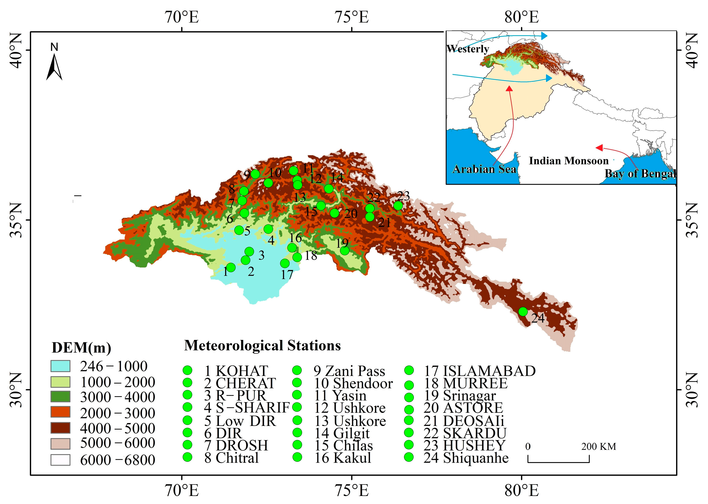
2.1. Study Area

The Indus River is one of the important rivers of the “Asian Water Tower”, whose upper basin is located in the northwestern part of the Tibetan Plateau and originates from the Hindu Kush-Karakorum-Himalayan region [30,37]. The entire river basin spans four countries: China, Pakistan, Afghanistan, and India. Its main tributary is located in Pakistan. The elevation of the basin ranges from 246 to 6800 m above sea level (a.s.l.), with almost 50% of the basin area having an elevation of more than 4000 m. It is one of the largest areas covered by glaciers (22,000 km²) due to its geographical location and complicated alpine land surface features, with an average multi-year snow cover of roughly 33–36% [38,39]. Nearly 80% of Pakistan’s irrigation water comes from snow and glacier meltwater, which together account for about 40.6% of the region’s runoff [40]. The variability of snow- and glacier-fed water is regarded as a key indicator of climate change, and it is crucial for the sustainable development of socio-economics and ecosystems in the middle and lower Indus Basin [41,42]. Precipitation in the UIB is affected by the interaction of the westerlies and the Indian monsoon [43]. The area’s climate has seen significant regional and seasonal changes, as evidenced by variations in temperature and precipitation. Due to the availability of data, 24 gauged meteorological stations were employed in the study; nevertheless, their distribution was uneven, with the majority of them being found in low-lying or flat areas (Figure 1). Therefore, obtaining high spatiotemporal resolution precipitation data is a requirement and a top priority for many UIB projects.

2.2. Data Collection and Processing

2.2.1. TRMM Precipitation Dataset

The joint U.S. and Japanese TRMM (1997–2015) endeavor used radar, microwave imaging and lightning sensors to detect rainfall and was aimed to reveal the distribution and variability of precipitation in tropical and subtropical rainfall [13]. Since the launch of the TRMM, it has supplied essential precipitation information for a range of scientific projects [14,44]. We obtained the TRMM3B42 precipitation dataset from the NASA official website (http://mirador.gsfc.nasa.gov (accessed on 13 January 2023)), the spatial resolution of 0.25° (approximately 27.75 km). Monthly and annual precipitation were formed by the accumulation of precipitation at different time intervals, respectively. Due to the availability of observed precipitation data, the time span of TRMM precipitation was determined from 2000 to 2017.

2.2.2. Precipitation Gauge Data

Daily recorded precipitation values from 2000 to 2017 of 24 meteorological gauge stations (8 meteorological stations with daily precipitation records for 2000 to 2013) located in Pakistan were obtained from Pakistan Metrological Department (PMD) and Pakistan Water and Power Development Authority (WAPDA). The spatial distribution and basic information of these meteorological gauge stations is shown in Figure 1 and

Table 1. Basic information about the observed meteorological stations used in the study.

Name	Agency	Longitude	Latitude	Elevation (m)	Annual Mean Precipitation (mm)	Period
ASTORE	PMD	74.9	35.37	2168	408.79	2000–2017
CHERAT	PMD	71.88	33.82	1372	635.51	2000–2017
CHILAS	PMD	74.1	35.42	1250	179.51	2000–2017
DIR	PMD	71.85	35.2	1375	1198.93	2000–2013
DROSH	PMD	71.783	35.57	1464	529.51	2000–2013
Chitral	PMD	71.83	35.85	1498	452.08	2000–2017
Gilgit	PMD	74.33	35.92	1460	148.79	2000–2017
Gupis	PMD	73.4	36.17	2156	234.23	2000–2017
ISLAMABAD	PMD	73.04	33.72	831	1215.75	2000–2017
Lower Dir	PMD	71.69	34.7	1375	835.57	2000–2017
KAKUL	PMD	73.3	34.18	1308	1159.29	2000–2013
KOHAT	PMD	71.43	33.55	513	564.38	2000–2013
MURREE	PMD	73.4	33.9	2291	1539.37	2000–2017
R-PUR	PMD	71.97	34.08	320	762.57	2000–2013
SKARDU	PMD	75.54	35.34	2267	233.86	2000–2013
S-SHARIF	PMD	72.35	34.82	970	988.24	2000–2013
Srinagar	PMD	74.8	34.1	1604	565.22	2000–2017
Shiquanhe	CIMISS	80.05	32.3	4280	67.53	2000–2013
Ushkore	WAPDA	73.42	36.03	3051	454.31	2000–2017
Yasin	WAPDA	73.29	36.45	3280	673.11	2000–2017
Zani Pass	WAPDA	72.17	36.35	3839	315.06	2000–2017
Deosai	WAPDA	75.54	35.09	4149	435.98	2000–2017
Hushey	WAPDA	76.37	35.42	3076	666.58	2000–2017
Shendoor	WAPDA	72.55	36.09	3712	408.18	2000–2017

. Nevertheless, the distribution of these gauge meteorological stations in the UIB is quite uneven; hence, it is impossible to collect precipitation data with high spatiotemporal resolution directly by the methods of interpolation. In this research, precipitation gauge data was used primarily for verifying the downscaled TRMM datasets based on the GWR model and S-GWR model.

2.2.3. Environmental Variables

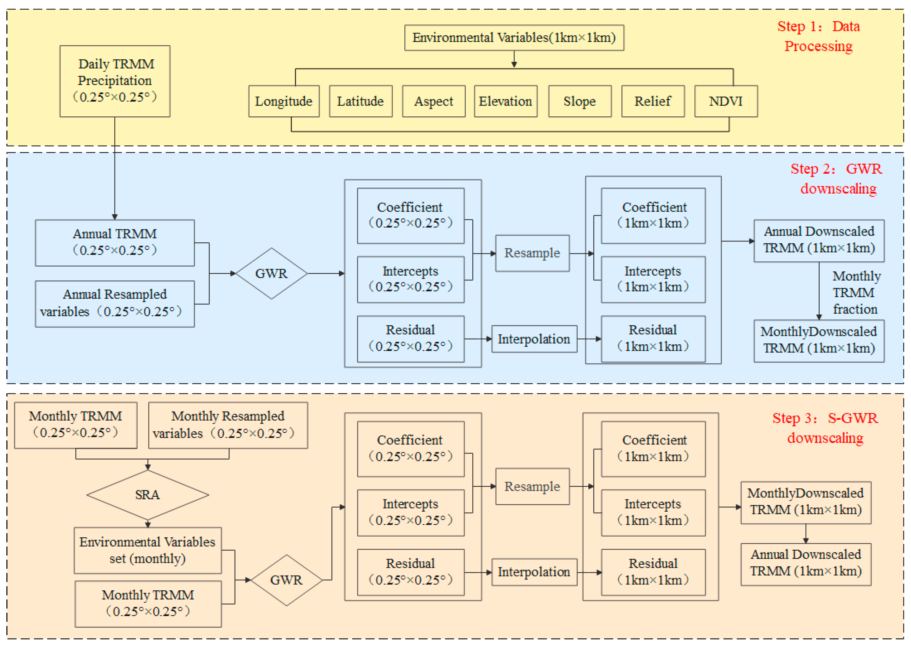
Digital elevation model (DEM) data, with the spatial resolution of 90 m, obtained from the Space Shuttle Radar Topography Mission (SRTM) (http://www.gscloud.cn (accessed on 13 January 2023)), was utilized to delineate geographical characters of aspect, slope, elevation and relief in this study. All these geographical layers were recognized as environmental variables. The monthly MODIS NDVI dataset (MOD13A3, 2000–2017) of the UIB, with a spatial resolution of 1 km, was derived from NASA (http://reverb.echo.nasa.gov/ (accessed on 13 January 2023)). Finally, Universal Transverse Mercator Grid System (WGS_1984_UTM_Zone_43N (accessed on 13 January 2023)) projected all the environmental variables, including latitude, longitude, elevation, slope, aspect, geographic relief and NDVI. All the utilized data were projected, extracted and aggregated based on the Python27.

2.3. Methods

The TRMM precipitation dataset was downscaled to a relatively high resolution (1 km × 1 km) by using both the stepwise regression analysis (SRA) and geographically weighted regression model (GWR) at monthly and annual scales. The technique of downscaling was accomplished based on two assumptions: (1) the spatial non-stationarity of TRMM (0.25° × 0.25°) precipitation can be explained by environmental variables; (2) high-resolution precipitation can be predicted using high-resolution environmental factors. The detailed technique of data downscaling is explained as follows (Figure 2):

(1) Data preparation. The original TRMM (0.25° × 0.25°) precipitation data and environmental variables (1 km × 1 km), which are required for model input, were prepared. The original TRMM data from January 2000 to December 2017 were aggregated on monthly and annual scales. Environmental variables include latitude, longitude, elevation, NDVI, slope, aspect and geographic relief. The same projection (WGS_1984_UTM_Zone_43N) was used to project the above datasets.

(2) The GWR model downscaling without environmental variable filtration (namely, GWR). Establish the GWR model between all environmental variables and the original TRMM datasets at annual scale for obtaining the intercepts, regression coefficients and residuals.

(3) Environmental variable filtration was executed first and followed by GWR model downscaling (namely, S-GWR). The SRA was used to filter environmental variables at monthly scale, and a total of 216 months from 2000 to 2017 were utilized for the SRA. This step eliminates irrelevant variables that may decrease the model performance and obtains the optimal environmental variables in each month. The environmental variables were resampled to 0.25° according to the resolution of the original TRMM datasets (0.25° × 0.25°). Establish the GWR model between environmental variables filtered by SRA and the original TRMM datasets at a monthly scale for obtaining the intercepts, regression coefficients and residuals.

(4) Regression parameter processing. The intercepts dataset and regression coefficient dataset from the GWR and S-GWR models were resampled to a high-resolution (1 km × 1 km), and the residual dataset is interpolated to 1 km by using the inverse distance weighting (IDW) method.

(5) Downscaled data achievement by the GWR model. The downscaled annual TRMM dataset (1 km × 1 km) was obtained based on Equation (3); all environmental variables were multiplied with the corresponding coefficients, and then added the corresponding constant terms and residuals. Disaggregation annual precipitation into monthly precipitation using a fraction disaggregation method based on Equation (6).

(6) Downscaled data achievement by the S-GWR model. The downscaled monthly TRMM dataset (1 km × 1 km) was obtained based on Equation (3); the filtered environmental variables in each month were multiplied with the corresponding coefficients, and then added to the corresponding constant terms and residuals.

2.3.1. The Stepwise Regression Analysis (SRA)

The SRA model can automatically filter the crucial variables from a large number of variables and develop predictive or explanatory models for regression analysis [45]. Hence, it can be used for reducing the impact of multicollinearity and for variables filtration. Since the correlations between precipitation and environmental variables vary in diverse times, the SRA approach was utilized to filter environmental variables that are considerably associated with precipitation at a corresponding monthly scale. The SRA normally removes the least important variables in a stepwise manner based on partial F-tests [46] until all remaining variables are statistically significant. The partial F-statistic is defined as follows:

$$F=\frac{\left(R_q^2-R_{q-1}^2\right)\left(n-q-1\right)}{\left(1-R_q^2\right)}$$

(1)

where $q$ is the number of predictors,$n-q-1$ is the degree of freedom, and $R$ indicates the correlation coefficient between precipitation and environmental variables in this study. When the p-value of the F test is less than 0.05, the environmental variables are removed; otherwise, it is retained.

The SRA model was established using the SPSS 26, with the TRMM precipitation data as the dependent variable and the environment variables as the independent variables. The equation of the SRA can be expressed as follows:

$$Y={\propto }_0+{\propto }_1{X}_1+{\propto }_2{X}_2+\cdots +{\propto }_i{X}_i$$

(2)

where $Y$ is the TRMM data, $X_i$ is the environment variable, and ${\propto }_i$ is the partial regression coefficient of each independent environment variables.

2.3.2. Geographically Weighted Regression Model (GWR)

Generally, most statistical models expect the relationships between result and predictor variables to be spatially constant. However, the GWR model establishes a local regression equation for each point in the spatial range [47]; thus, it is the regression algorithm that takes into account the non-stationary relationship between the predictor and outcome variables [48]. Equation (3) can be used to establish the GWR model as

$$Y_i={\beta }_0\left(u_i,v_i\right)+{\displaystyle \sum _{k=1}^p}{\beta }_i\left(u_i,v_i\right)X_{ik}+{\epsilon }_i$$

(3)

where $\left(u_i,v_i\right)$ denote the spatial position of the$i$; ${\beta }_0\left(u_i,v_i\right)$ and ${\beta }_i\left(u_i,v_i\right)$ are the intercept and slope at point I, respectively; ${\mathsf{\epsilon }}_i$ is the regression residual at point $i$, P denotes the number of predictor variables. Unlike the conventional global regression model, the GWR model is established based on the assumption that the sample points have greater impacts on the prediction point that is closer to it; and the model adopts a function that the weight decays with the distance of the sample from the predicted point increases, so the coefficient changes in space. The coefficient is calculated as:

$$\widehat{\beta }\left(u_i,v_i\right)={\left(X^T\left(W\left(u_i,v_i\right)\right)X\right)}^{-1}{X}^{T}W\left(u_i,v_i\right)Y$$

(4)

where $\widehat{\beta }\left(u_i,v_i\right)$is the parameter estimate at the point $\left(u_i,v_i\right)$; X and Y are the vector sets of predictor and outcome variables, respectively. $W\left(u_i,v_i\right)$ is the weight matrix, which serves to ensure that the modeling points which are closer to the location of the point $i$ have a greater weight in estimating the parameter of the point $i$. The weight allocation follows the formula below:

$$\begin{array}{c}{w}_{i,j}=\left\{\begin{array}{c}{\left(1-\frac{d_{ij}^2}{{\theta }_{i\left(k\right)}}\right)}^2,d_{ij}\le D\\ 0,d_{ij}>D\end{array}\right.\end{array}$$

(5)

where$d_{ij}$ is the Euclidean distance between the j point and $i$ point;$D$ is the radius of the kernel weight function. Adaptive Bi-square and the Akaike information criterion (AICc) are chosen as the kernel weight function and the bandwidth, respectively, which have the best effect in estimating precipitation [49].

2.3.3. Disaggregation of Annual Precipitation

$$Fra{c}_i=\frac{P_{TRMMi}}{{{\displaystyle \sum }}_{i=1}^{12}{P}_{TRMMi}}$$

(6)

where$P_{TRMMi}$ represents the original TRMM data of the $i$th month, and the denominator represents the annual TRMM data obtained by accumulating monthly original TRMM precipitation data.

2.3.4. Performance of Variables Filtration and Data Downscaling

The accuracy of the TRMM precipitation data was assessed according to correlation coefficient (R), relative error index (BIAS) and root mean square error (RMSE). R reflects the linear correlation between two sets of data. BIAS describes the extent to which predicted data overestimate or underestimate when compared with the observed data. RMSE denotes the overall level of error in predicting data. The corresponding equations of these indicators are as follows:

$$R=\frac{{{\displaystyle \sum }}_{i=1}^n\left(x_i-\overline{x}\right)\left(y_i-\overline{y}\right)}{\sqrt{{{\displaystyle \sum }}_{i=1}^n{\left(x_i-\overline{x}\right)}^2}{{\displaystyle \sum }}_{i=1}^n{\left(y_i-\overline{y}\right)}^2}$$

(7)

$$BIAS=\frac{{{\displaystyle \sum }}_{i=1}^n{x}_i}{{{\displaystyle \sum }}_{i=1}^n{y}_i}-1$$

(8)

$$RMSE=\sqrt{\frac{{{\displaystyle \sum }}_{i=1}^n{\left(x_i-y_i\right)}^2}{n}}$$

(9)

where$x_i$, $y_i$ are TRMM data and observation precipitation data measured by rain gauge, respectively; $\overline{x},\overline{y}$ are the mean value of TRMM data and observation precipitation data, respectively; n is the total number of meteorological gauge stations in the UIB (n = 24).

3. Results

3.1. Environmental Variables Filtration

The correlations between environmental variables and precipitation could be used to recognize the dominant factors that influence the precipitation variability in the UIB. Figure 3 represents the results of environmental variables filtration at a monthly scale by the SRA model from January 2000 to December 2017 (216 months in total). There are three environmental variables that are the most frequent variables which influence the downscaling the most (85 occurrences in 216 months, Figure 3a). In terms of the variable types, elevation, longitude, NDVI and latitude are the most frequent variables (frequency varies from 143 to 183 times) which explain the variability of precipitation, whereas aspect is the least frequent variable (Figure 3b).

The numbers of environmental variables distributed in each month are given in Figure 3c. The results of correlation between longitude and precipitation suggest relatively good correlation during all the months, and the numbers of this variable did not fluctuate too much throughout the whole year. The latitude variable indicates an enhanced connection with precipitation in October and November. The NDVI variable is mostly related to precipitation in spring (March–May) and decreases dramatically in summer. The slope and aspect vary less due to the small numbers after the SRA filtration, but the numbers of the slope increase in August. Aspect is more explanatory of precipitation in May. Topographic relief contributed less throughout the year, except for an increase in July and August. The contribution of elevation is higher throughout the year, especially from June to September.

3.2. Comparative Evaluation of the Accuracy of Downscaled TRMM Data with GWR and S-GWR Models

To evaluate the effect of variable filtration on downscaling, the downscaled TRMM data based on the GWR model and S-GWR model were both compared with 24 precipitation stations with the help of statistical tests at temporal and spatial scales across the UIB.

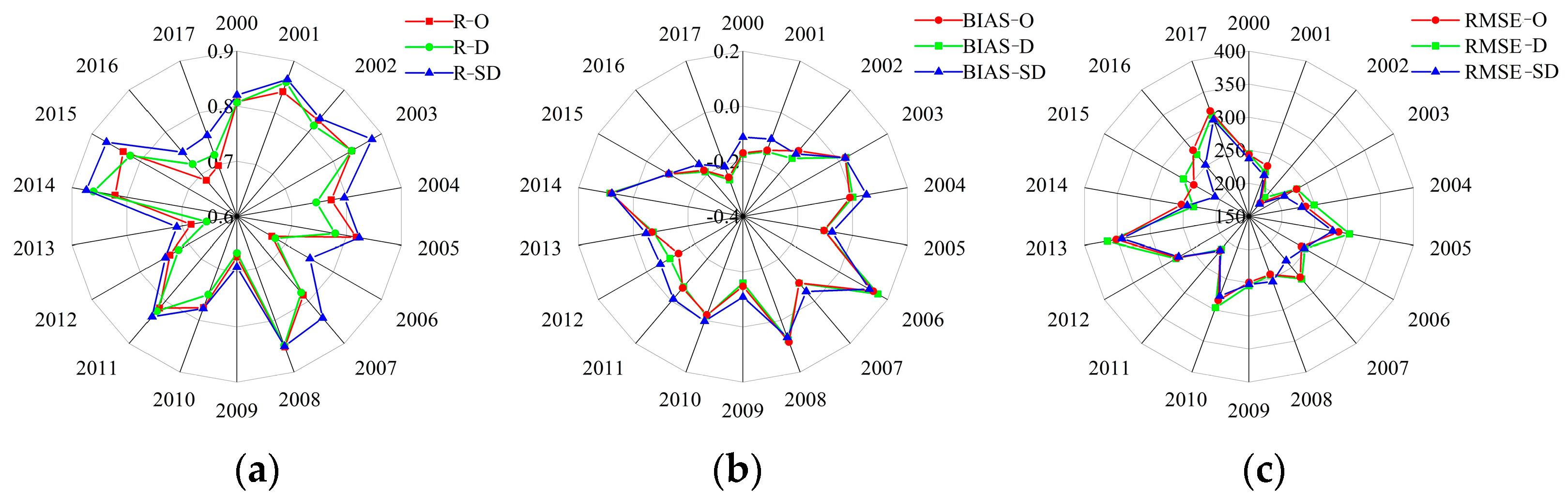
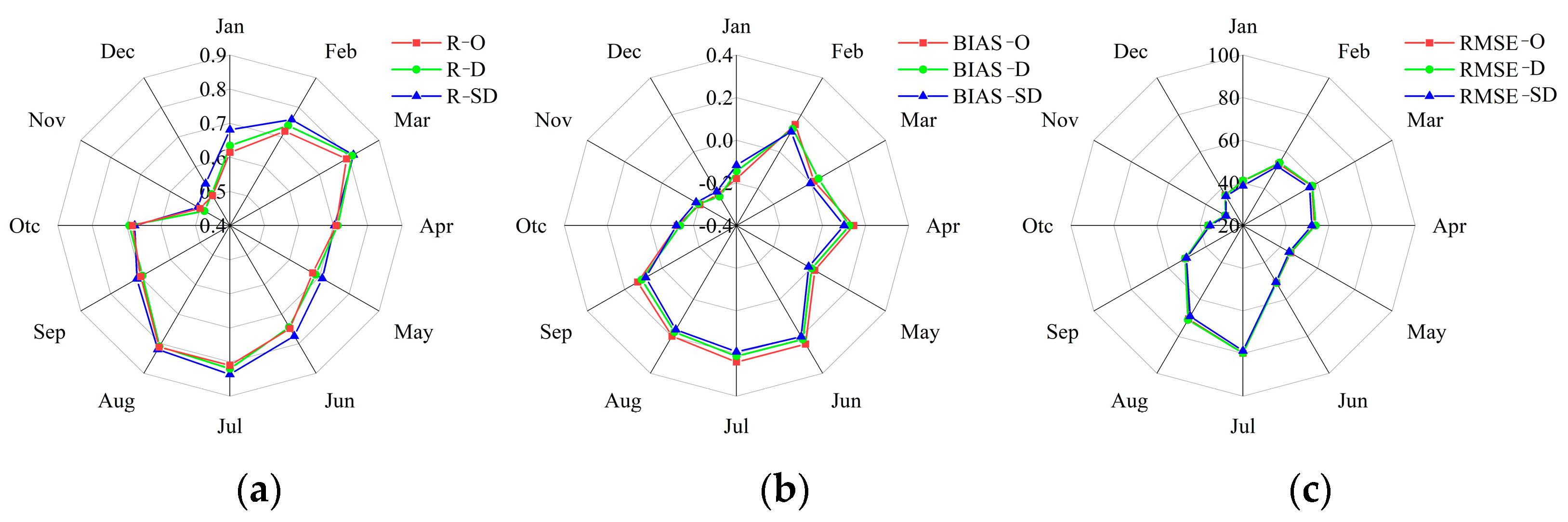
3.2.1. Temporal Scale Evaluation

Annual and monthly validation of the original TRMM and TRMM data downscaled by the GWR model and S-GWR model that compared with the observed data are presented in Figure 4 and Figure 5, respectively. Annually, the TRMM data downscaled by the S-GWR model generally displays a better correlation than the original TRMM data and GWR downscaled TRMM with the observations (Figure 4a), the R values were improved in each year and multi-year average (2000–2017) of R was improved from 0.77 to 0.8. Biases of all the years are below 0.2, except for 2017 when the BIAS is −0.21. Nonetheless, the BIAS of the TRMM data downscaled by the S-GWR model is smaller than that of the original TRMM data and the TRMM data downscaled by the GWR model (Figure 4b). Compared with the observed precipitation, the RMSE of the downscaled TRMM data is smaller than that of the original TRMM data, but the RMSE is still kind of large (Figure 4c). Generally, the BIAS and RMSE are more or less identical before and after downscaling, the BIAS and RMSE of TRMM data downscaled after variables filtration were reduced.

Overall, the correlations between the observed precipitation and downscaled TRMM data are still stronger than those with the original TRMM data in all months. The R between the observed precipitation data and both of the before and after downscaled TRMM data are generally higher in the summer months (June to August, R > 0.8), notably, the R in November and December (the R was distributed between 0.5 to 0.6, respectively) were relatively lower than in other months. The R between the downscaled TRMM data and the observed data is the highest in July (R = 0.83) (Figure 5a). Contrary to the distribution of R in November and December, the BIAS in November and December are around 0.2. However, both of the original and downscaled TRMM data overestimated precipitation in the months from June to September (BIAS > 0) (Figure 5b). Additionally, the RMSE indicates strong variations in different months (Figure 5c). The RMSE is considerably lower in the winter (December to February) and spring months (March to May) than that in the summer months, especially in July and August (78 mm and 69 mm, respectively) when it is the main rainy season in the UIB. Generally, the RMSE is more or less similar before and after downscaling, the RMSE of the TRMM data downscaled by S-GWR is smaller than the original TRMM data and GWR downscaled TRMM in all months.

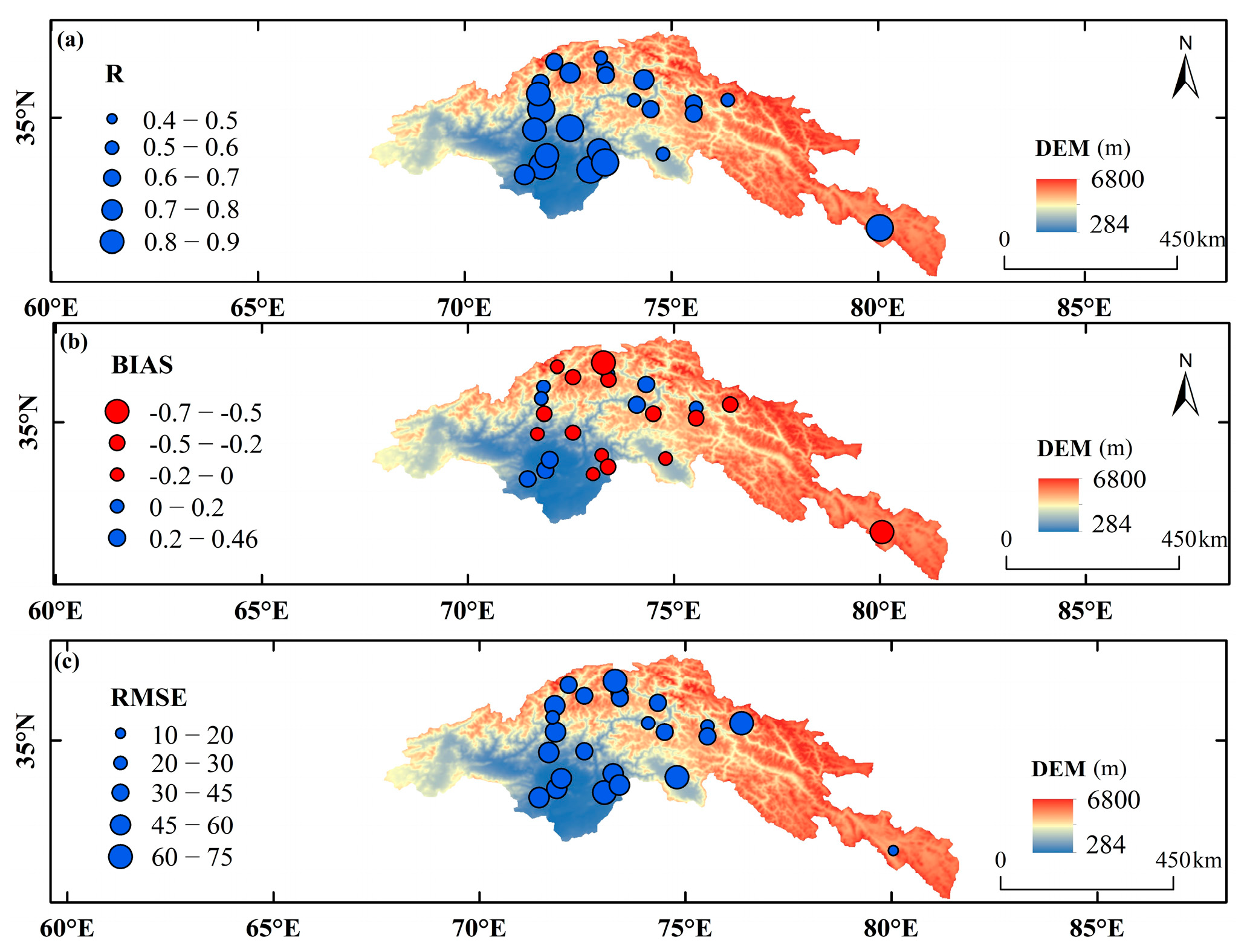
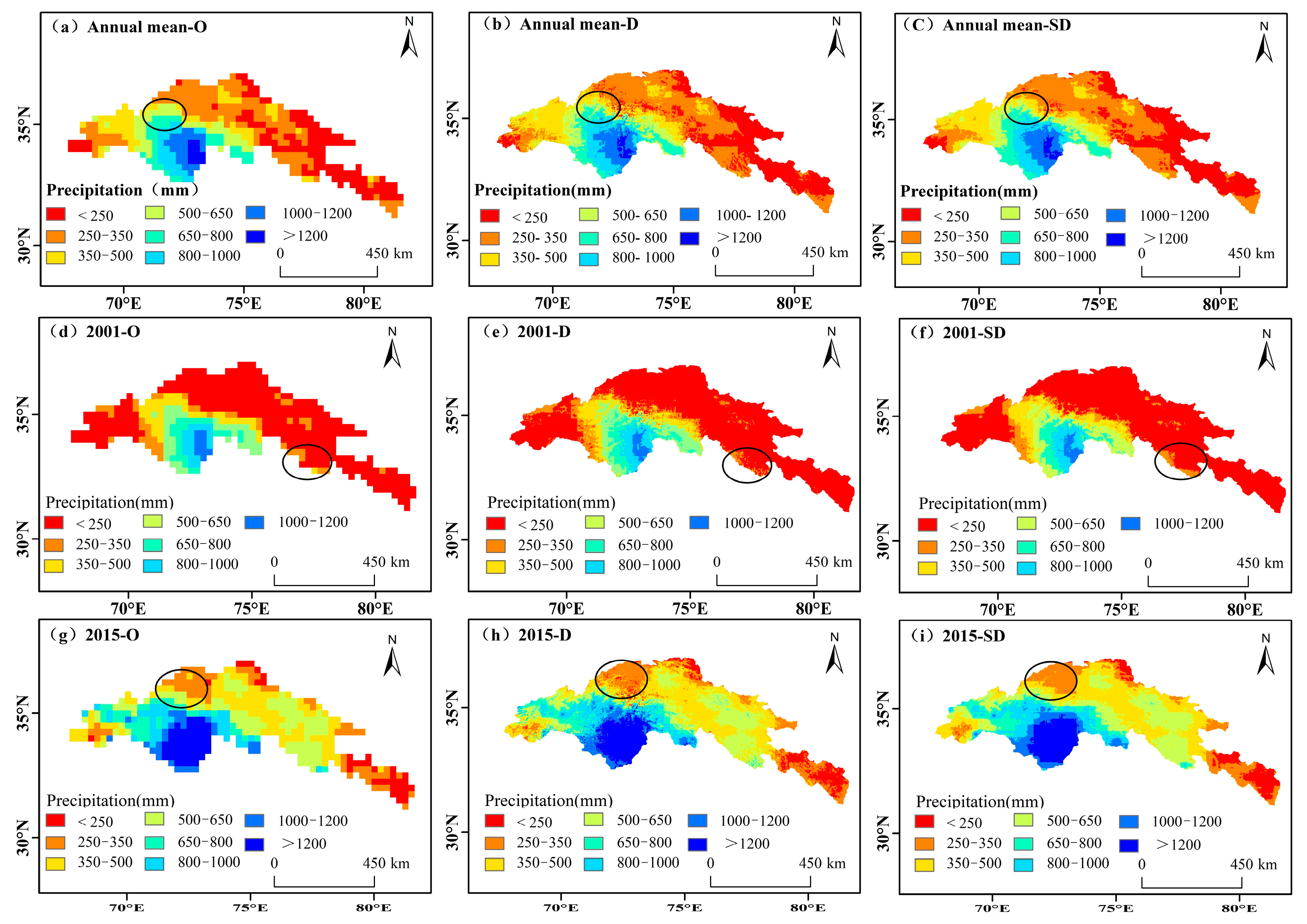
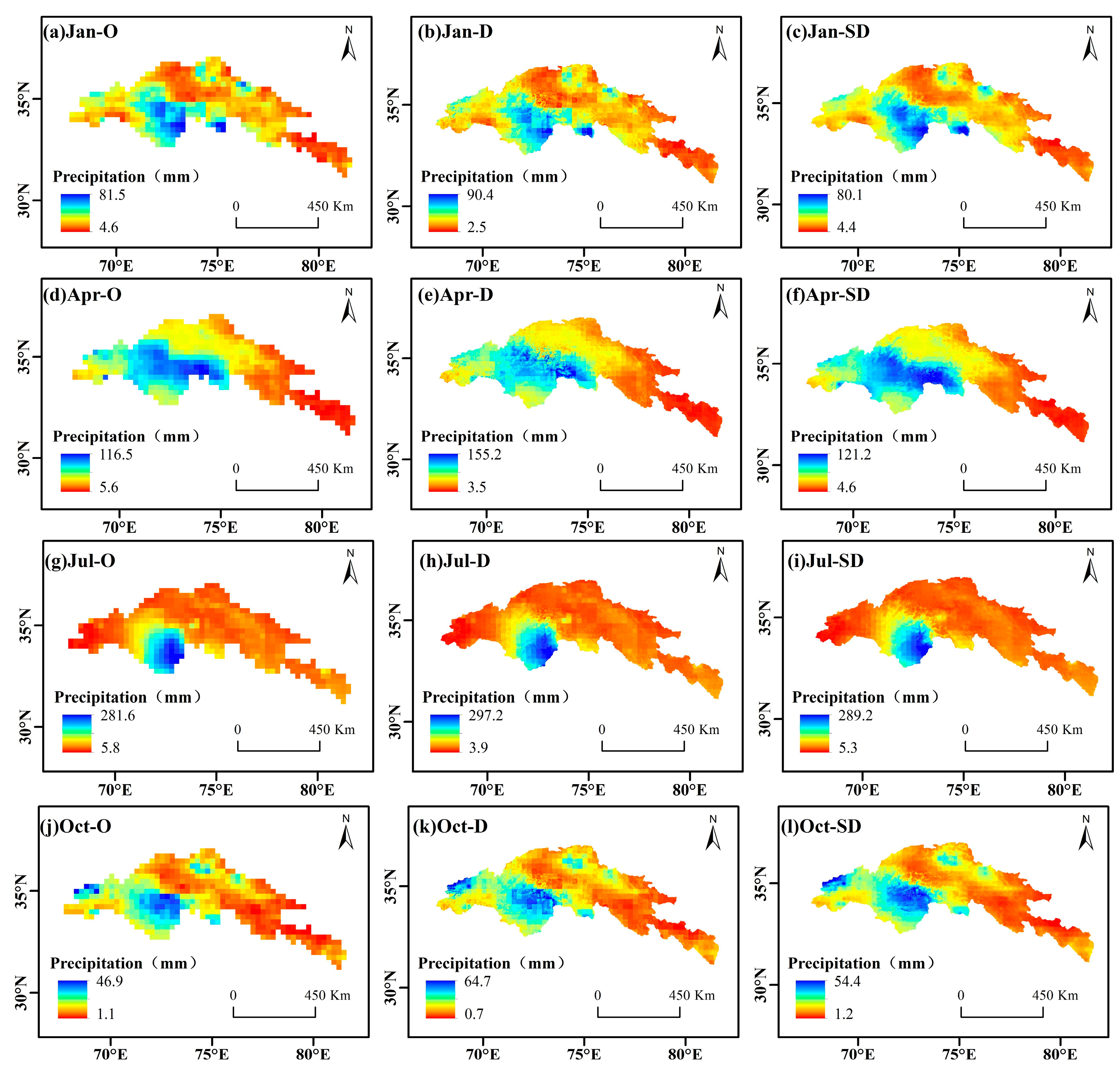
3.2.2. Spatial Scale Evaluation

The original and downscaled TRMM data by the GWR model and S-GWR model at 24 observed weather stations were extracted and compared directly with the corresponding observational data in terms of the evaluation indicators. Overall, the accuracy of the downscaled TRMM data is better than the original TRMM data at all the meteorological stations, except for the ASTORE, DIR and R-PUR stations (

Table 2. The R, BIAS, and RMSE of the observed and TRMM precipitation at each meteorological station in the UIB.3.3. The downscaling results of TRMM precipitation datasets.

Stations	R			BIAS			RMSE(mm)
	O	GWR	S-GWR	O	GWR	S-GWR	O	GWR	S-GWR
ASTORE	0.58	0.57	0.56	−0.27	−0.23	−0.28	31.11	31.44	31.59
CHERAT	0.74	0.76	0.83	0.42	0.31	0.34	56.00	49.06	45.62
Chitral	0.15	0.15	0.52	0.26	0.34	0.16	57.35	59.35	57.90
CHILAS	0.38	0.35	0.49	0.49	0.51	0.46	27.15	27.50	26.41
DIR	0.87	0.86	0.83	−0.38	−0.30	−0.28	55.68	50.79	48.63
DROSH	0.72	0.71	0.78	0.27	0.12	0.14	28.92	27.06	26.78
Gilgit	0.48	0.49	0.62	0.85	0.46	0.36	33.64	27.76	30.52
Gupis	0.27	0.25	0.59	0.17	0.18	0.15	32.90	33.55	31.96
M-ABAD	0.85	0.85	0.85	0.01	−0.03	−0.07	73.28	73.25	73.63
KOHAT	0.53	0.62	0.62	0.41	0.54	0.37	52.91	58.26	51.90
KAKUL	0.72	0.72	0.78	−0.03	−0.09	−0.07	49.55	50.12	48.50
Lower dir	0.50	0.50	0.75	0.04	−0.02	0.02	89.13	86.88	48.05
MURREE	0.84	0.84	0.89	−0.24	−0.40	−0.40	71.40	87.81	55.58
R-PUR	0.78	0.78	0.75	0.36	0.38	0.36	52.73	50.09	51.83
S-SHARIF	0.77	0.77	0.83	0.25	−0.22	−0.20	57.06	40.25	40.47
Srinagar	0.23	0.36	0.42	0.04	0.05	0.04	66.27	66.31	66.25
SKARDU	0.48	0.55	0.54	−0.32	0.11	0.21	20.17	21.10	20.17
Shiquanhe	0.79	0.78	0.82	−0.72	−0.73	−0.71	10.36	9.51	9.09
Ushkore	0.12	0.19	0.51	−0.44	−0.46	−0.43	44.46	43.27	44.90
Yasin	0.15	0.11	0.47	−0.58	−0.56	−0.56	74.50	75.36	74.81
Zani Pass	0.44	0.47	0.55	−0.15	0.13	0.05	36.43	42.10	37.34
Deosai	0.27	0.27	0.59	−0.44	−0.44	−0.41	39.48	39.32	38.36
Hushey	0.39	0.40	0.49	−0.47	−0.43	−0.43	60.07	59.84	60.30
Shendoor	0.32	0.33	0.60	−0.31	−0.24	−0.25	43.41	43.68	42.69

). Additionally, the spatial performance of the S-GWR model downscaled TRMM data at each site was reported in Figure 6. In terms of the correlation between the downscaled TRMM data and the observational data, the mean R is 0.65 and the R spans from 0.47 (the Yasin station) to 0.89 (the MURREE station). However, the sites at lower elevations generally have higher correlations with the observed precipitation than that at higher elevations (Figure 6a). In addition, the BIAS of the downscaled TRMM data ranged from −0.56 (the ASTORE station) to 0.71 (the Shiquanhe station) and relatively large negative BIAS was typically detected in places with high precipitation (Figure 6b). Generally, the TRMM precipitation data underestimate high precipitation while overestimating low precipitation in the UIB. Similarly, the RMSE (9–74 mm) is higher in the locations which are located at low elevations yet with high precipitation (Figure 6c).

To explore the result of spatial downscaling, both of the original TRMM data and S-GWR model downscaled TRMM data were generated for the average of study period 2000–2017 and different climate years 2001 (dry year, annual average precipitation is 301 mm) and 2015 (wet year, annual precipitation is 622 mm) in the UIB (Figure 7). Average annual precipitation (435 mm) varies widely (11–1296 mm) across the UIB due to topography and moisture sources, presenting an increasing feature from northeast to southwest (Figure 7a–c). Generally, the original TRMM data has a mosaic distribution due to its coarse resolution; undoubtedly, both downscaled TRMM data maintained the spatial patterns and improved the expression of the spatial information. However, the S-GWR model downscaled TRMM data was more consistent with original TRMM data, and the spatial variation exhibits a clearer pattern in both the climatic years, especially in the high elevations with little precipitation (black circles drawn over some regions in Figure 7).

Figure 8 shows the spatial distribution of the original and downscaled TRMM data by the GWR and S-GWR model in typical months from 2000 to 2017. Compared with the original TRMM data, both the downscaled TRMM data has improved spatial resolution in all the months, and the spatial distribution is more refined, which can better represent the patterns of the local precipitation. However, these two models’ downscaled TRMM data are similar in spatial distribution at the monthly scale.

4. Discussion

4.1. Environmental Variables Filtration

Less environmental variables, such as NDVI and DEM, may not meet the requirements of collaborative inversion of high-resolution precipitation under the influence of multiple variables [35,36]. When all the variables relating to the land-surface environment are taken into account, multicollinearity problems could also be present. As a result, filtering environmental variables should come before downscaling [50]. Based on the SRA model, we explore the non-stationarity [49] of the interactions between precipitation and environmental variables in this work. The SRA model has the advantage of retaining the variables with the greatest influence as suggested by Teegavarapu and Goly [51] and can be used for variables filtration. We discovered that there is spatiotemporal variability in the associations between precipitation and variables, which is different from studies that do not consider the monthly relationships between precipitation and environmental factors. Further research should address both the spatial and temporal aspects of the non-stationarity connections because different environmental variables have varied effects during different months (216 months in total, Figure 3c) [35,36,49].

The most frequent factors to explain the variability in precipitation in the UIB are elevation, longitude, NDVI, and latitude, whereas aspect is the least frequent variable. This is essentially compatible with the findings of Wang et al. [52], despite the fact that NDVI was excluded from their study. Because the UIB has a significant elevation change, the elevation has a significant influence in the downscaling. The elevation decreases from northeast to southwest, while the precipitation shows the opposite trend that increases from northeast to southwest. This pattern is mainly influenced by climatic systems which are also influenced by the geographical characteristics of elevation, longitude and latitude. Studies have shown that westerly winds dominate in the northeastern part of the UIB, with westerly transport accounting for 70% of precipitation [43]. However, the Indian monsoon has an impact on the UIB’s southeast region, so the water vapor there primarily comes from the Indian Ocean and Bay of Bengal [43]. Additionally, because vegetation responds immediately to precipitation and is affected by variations in temperature and humidity, it is possible to explain precipitation using NDVI at a monthly scale [53]. As a result, there is a fair amount of correlation between elevation, longitude, NDVI, and fluctuations in precipitation across time in the UIB.

The fact that summer precipitation is mostly regulated by the monsoon, whereas spring and winter precipitation is primarily regulated by westerly winds, may explain why environmental factors vary dramatically in summer [43]. The Indian summer monsoon’s vigor primarily determines the season’s precipitation. More moisture was present on the southern slope as a result of the Karakoram Mountains blocking water vapor from the southwest [54]. Due to the abrupt change in topography in the western part of the Himalayas, water vapor from the Arabian Sea and the Bay of Bengal creates intense topographic rainfall that exceeds 1000 mm/year in the southwestern part of the basin [55,56,57]. The extension of water vapor also exhibits a progressive decreasing pattern from the southwest to the northeast, which is obstructed by the Himalayas (Figure 7). The circulation is affected dynamically and thermally by plateau blockage and topographic friction. As a result, there is a strong link between elevation, longitude, latitude and monthly precipitation in the UIB.

4.2. TRMM Data Downscaling in the UIB

Existing studies have shown that the TRMM precipitation data outperformed other gridded precipitation products in the UIB [31,32], so the TRMM data was selected for downscaling, and we believed that this dataset is applicable in the UIB even though there are fewer observational data for evaluation due to data availability. After comparative analysis of the relationships between observed stations and the original TRMM data and downscaled TRMM data by GWR and S-GWR models, we found that the annual and monthly of downscaled precipitation by S-GWR model has higher correlations with the observed stations than that with the original TRMM data and GWR model downscaled TRMM data. Generally, the downscaling of environmental variables is a crucial step to improve the downscaling accuracy of gridded data, which is compatible with the findings of Wang et al. (2022) [52]. Additionally, Arshad et al. (2021) [33] applied a Mixed Geographically Weighted Regression (MGWR) model to downscale precipitation in the UIB. Although the spatial distribution characteristics of the downscaled TRMM data remained unaltered, it has more spatial information and higher resolution. However, the correlations between the downscaled TRMM precipitation data and the observed data are considerably lower than those found by Arshad et al. (2021) [33], which may be due to the different observed stations, different time periods and different non-stationary relations that were employed. We also found that the TRMM data failed to capture the peak of precipitation, especially at high elevations, which is consistent with the finding that the reliability of the original TRMM data is essential to the success of downscaling [21,49]. Because the objective of this study was to downscale the TRMM data based on the non-stationary relations at monthly scale, we did not include calibration after downscaling. However, research suggested that bias correction after downscaling could be another option for retrieving high-resolution precipitation data [33,34]. Additionally, other investigations discovered that despite the original TRMM data having relative higher relationship with observed data, the TRMM data either overestimated precipitation in alpine mountains regions [26] or overestimated precipitation at the daily scale [58]. Therefore, more research is needed on the spatiotemporal accuracy and downscaling of the TRMM data.

4.3. Uncertainty Analysis and Future Directions

The retrieval of high spatiotemporal resolution precipitation is still the bottleneck problem in the data-scarce mountainous region [35,52]. We tried to downscale the TRMM data by using both the SRA model and the GWR model for environmental variables filtration and data downscaling in the UIB, respectively. Although the filtration of environmental variables and downscaled TRMM data produced reasonably trustworthy results, uncertainties remain during these processes. Although geographical location and topographic factors were taken into account during variable filtration and data downscaling, however, there are some other environmental variables (e.g., surface temperature, soil moisture, cloud cover and wind speed etc.) that may also influence the variability of the precipitation [33,59,60,61]. Thus, different environmental variables might lead to different downscaling results.

Additionally, more observed stations are desperately needed for downscaling of precipitation data in the UIB, especially in the high mountainous region. Some high elevation stations are not yet available due to data scarcity in this study. Because most of the stations are in low elevations in the southwestern part of the UIB and have relatively short time periods, they cannot fully represent the variability of precipitation. This may be the cause of the study’s lower correlations and higher RMSE. We acknowledge that uncertainties remain.

Precipitation and environmental variables were shown to have yearly and multi-year average stationary relationships in earlier research [21,33]. Inspired by Xu et al. [49], we selected the environmental variables using a monthly downscaling algorithm based on the SRA in the UIB from 2000 to 2017. This allowed us to identify non-stationary relationships between precipitation and environmental variables and to determine the ideal set of variables for each month within the study area. However, because of the complex interactions between the land and atmosphere in this mountainous region, atmospheric factors such as atmospheric circulation pattern, wind direction and wind speed etc. may also contribute to increasing the accuracy of downscaling in the future. The results of this work will aid in hydrological studies in the UIB region, and the methods can be applied to other mountainous regions that require more precise precipitation data.

5. Conclusions

This study introduced environmental variables filtration developed for the downscaling of both monthly and yearly TRMM precipitation data in the range of 0.25° to 1 km. Environmental variables were filtered first based on the SRA model, and later downscaling took into consideration the non-stationary relationships between precipitation and environmental variables at each month. We also assessed the TRMM data’s accuracy with respect to the observed precipitation before and after downscaling. Overall, there were three or four variables, which are the most frequent variables that participated in the downscaling process of the UIB. The variables that might explain the variation in precipitation are elevation, longitude, NDVI and latitude, while aspect is the variable that occurs the least frequently after the variables filtration. In terms of the evaluation indicators (R, BIAS and RMSE), the downscaled TRMM data by the S-GWR model has relative higher accuracy than the original and GWR model downscaled TRMM data, and it offers more spatial information at a higher resolution in the UIB. Additionally, we find that the correctness of the original TRMM data strongly influences the findings of the downscaled TRMM data; hence, data evaluation and additional bias correction should be taken into account for lowering uncertainty. This study showed that additional research is urgently required to address the non-stationary interactions between precipitation and variables at various scales, even if uncertainties still exist due to the lack of data. The integrated variable filtration and data downscaling method may generally be used to successfully increase the spatial estimation of gridded precipitation at monthly and annual scales over the UIB, and it can be significant for other data downscaling research in mountain regions abroad.

References

1. Shen, Y.-J.; Shen, Y.J.; Fink, M.; Kralisch, S.; Brenning, A. Unraveling the hydrology of the glacierized Kaidu Basin by integrating multisource data in the Tianshan Mountains, Northwestern China. Water Resour. Res. 2018, 54, 557–580. [Google Scholar] [CrossRef]
2. Guo, Y.H.; Zhang, Y.Q.; Zhang, L.; Wang, Z. Regionalization of hydrological modeling for predicting streamflow in ungauged catchments: A comprehensive review. Wiley Interdiscip. Rev. Water 2020, 8, 32. [Google Scholar] [CrossRef]
3. Goovaerts, P. Geostatistical approaches for incorporating elevation into the spatial interpolation of rainfall. J. Hydrol. 2000, 228, 113–129. [Google Scholar] [CrossRef]
4. Guo, J.Z.; Liang, X.; Leung, L.R. Impacts of different precipitation data sources on water budgets. J. Hydrol. 2004, 298, 311–334. [Google Scholar] [CrossRef]
5. Langella, G.; Basile, A.; Bonfante, A.; Terribile, F. High-resolution space–time rainfall analysis using integrated ANN inference systems. J. Hydrol. 2010, 387, 328–342. [Google Scholar] [CrossRef]
6. Jiang, S.H.; Ren, L.L.; Hong, Y.; Yong, B.; Yang, X.; Yuan, F.Y.; Ma, M.W. Comprehensive evaluation of multi-satellite precipitation products with a dense rain gauge network and optimally merging their simulated hydrological flows using the Bayesian model averaging method. J. Hydrol. 2012, 452–453, 213–225. [Google Scholar] [CrossRef]
7. Shen, Y.-J.; Shen, Y.J.; Guo, Y.; Zhang, Y.C.; Pei, H.W.; Brenning, A. Review of historical and projected future climatic and hydrological changes in mountainous semiarid Xinjiang (northwestern China), central Asia. Catena 2019, 187, 104343. [Google Scholar] [CrossRef]
8. Collischonn, B.; Collischonn, W.; Tucci, C.E.M. Daily hydrological modeling in the Amazon basin using TRMM rainfall estimates. J. Hydrol. 2008, 360, 207–216. [Google Scholar] [CrossRef]
9. Qin, R.Z.; Zhao, Z.Y.; Xu, J.; Ye, J.S.; Li, F.M.; Zhang, F. HRLT: A high-resolution (1 d, 1 km) and long-term (1961–2019) gridded dataset for surface temperature and precipitation across China, Earth Syst. Sci. Data 2022, 14, 4793–4810. [Google Scholar] [CrossRef]
10. Huffman, G.J.; Adler, R.F.; Arkin, P.; Arkin, P.; Chang, A.; Ferraro, R.; Gruber, A.; Janowiak, J.; McNab, A.; Rudolf, B.; et al. The Global Precipitation Climatology Project (GPCP) combined precipitation dataset. Bull. Am. Meteorol. Soc. 1997, 78, 5–20. [Google Scholar] [CrossRef]
11. New, M.; Hulme, M.; Jones, P. Representing twentieth century space–time climate variability. Part 2: Development of 1901–96 monthly grids of terrestrial surface climate. J. Clim. 2000, 13, 2217–2238. [Google Scholar] [CrossRef]
12. Yatagai, A.; Kamiguchi, K.; Arakawa, O.; Hamada, A.; Yasutomi, N.; Kitoh, A. APHRODITE: Constructing a Long-Term Daily Gridded Precipitation Dataset for Asia Based on a Dense Network of Rain Gauges. Bull. Am. Meteorol. Soc. 2012, 93, 1401–1415. [Google Scholar] [CrossRef]
13. Kummerow, C.; Barnes, W.; Kozu, T.; Shiue, J.; Simpson, J. The Tropical Rainfall Measuring Mission (TRMM) Sensor Package. J. Atmos. Ocean. Technol. 1998, 15, 809–817. [Google Scholar] [CrossRef]
14. Yang, N.; Zhang, K.; Hong, Y.; Zhao, Q.H.; Huang, Q.; Xu, Y.; Xue, X.W.; Chen, S. Evaluation of the TRMM multisatellite precipitation analysis and its applicability in supporting reservoir operation and water resources management in Hanjiang basin, China. J. Hydrol. 2017, 549, 313–325. [Google Scholar] [CrossRef]
15. Gao, Y.C.; Liu, M.F. Evaluation of high-resolution satellite precipitation products using rain gauge observations over the Tibetan Plateau. Hydrol. Earth Syst. Sci. 2013, 17, 837–849. [Google Scholar] [CrossRef]
16. Nastos, P.T.; Kapsomenakis, J.; Philandras, K.M. Evaluation of the TRMM 3B43 gridded precipitation estimates over Greece. Atmos. Res. 2016, 169, 497–514. [Google Scholar] [CrossRef]
17. Tao, K.; Barros, A.P. Using Fractal Downscaling of Satellite Precipitation Products for Hydrometeorological Applications. J. Atmos. Ocean. Technol. 2010, 27, 409–427. [Google Scholar] [CrossRef]
18. Abdollahipour, A.; Ahmadi, H.; Aminnejad, B. A review of downscaling methods of satellite-based precipitation estimates. Earth Sci. Inform. 2021, 15, 1–20. [Google Scholar] [CrossRef]
19. Murphy, J. Predictions of climate change over Europe using statistical and dynamical downscaling techniques. Int. J. Climatol. 2000, 20, 489–501. [Google Scholar] [CrossRef]
20. Zhang, Y.Y.; Li, Y.G.; Ji, X.; Luo, X.; Li, X. Fine-Resolution Precipitation Mapping in a Mountainous Watershed: Geostatistical Downscaling of TRMM Products Based on Environmental Variables. Remote Sens. 2018, 10, 119. [Google Scholar] [CrossRef]
21. Immerzeel, W.W.; Rutten, M.M.; Droogers, P. Spatial downscaling of TRMM precipitation using vegetative response on the Iberian Peninsula. Remote Sens. Environ. 2009, 113, 362–370. [Google Scholar] [CrossRef]
22. Huth, R.; Kliegrová, S.; Metelka, L. Non-linearity in statistical downscaling: Does it bring an improvement for daily temperature in Europe? Int. J. Climatol. 2008, 28, 465–477. [Google Scholar] [CrossRef]
23. Shi, Y.L.; Song, L. Spatial downscaling of monthly TRMM precipitation based on EVI and other geospatial variables over the Tibetan Plateau from 2001 to 2012. Mt. Res. Dev. 2015, 35, 180–194. [Google Scholar] [CrossRef]
24. Jing, W.L.; Yang, Y.P.; Yue, X.F.; Zhao, X.D. A comparison of different regression algorithms for downscaling monthly satellite-based precipitation over north China. Remote Sens. 2016, 8, 835. [Google Scholar] [CrossRef]
25. Chen, C.; Zhao, S.H.; Duan, Z.; Qin, Z.H. An Improved Spatial Downscaling Procedure for TRMM 3B43 Precipitation Product Using Geographically Weighted Regression. IEEE J. Sel. Top. Appl. Earth Obs. Remote Sens. 2015, 8, 4592–4604. [Google Scholar] [CrossRef]
26. Chen, F.R.; Liu, Y.; Liu, Q.; Li, X. Spatial downscaling of TRMM 3B43 precipitation considering spatial heterogeneity. Int. J. Remote Sens. 2014, 35, 3074–3093. [Google Scholar] [CrossRef]
27. Chen, S.L.; Xiong, L.H.; Ma, Q.M.; Kim, J.S.; Chen, J.; Xu, C.Y. Improving daily spatial precipitation estimates by merging gauge observation with multiple satellite-based precipitation products based on the geographically weighted ridge regression method. J. Hydrol. 2020, 589, 125156. [Google Scholar] [CrossRef]
28. Sun, X.N.; Wang, J.C.; Zhang, L.W.; Ji, C.J.; Zhang, W.; Li, W.K. Spatial Downscaling Model Combined with the Geographically Weighted Regression and Multifractal Models for Monthly GPM/IMERG Precipitation in Hubei Province, China. Atmosphere 2022, 13, 476. [Google Scholar] [CrossRef]
29. Zhao, Z.Q.; Gao, J.B.; Wang, Y.L.; Liu, J.G.; Li, S.C. Exploring spatially variable relationships between NDVI and climatic factors in a transition zone using geographically weighted regression. Theor. Appl. Climatol. 2014, 120, 507–519. [Google Scholar] [CrossRef]
30. Lutz, A.F.; Immerzeel, W.W.; Kraaijenbrink, P.D.A.; Shrestha, A.B.; Bierkens, M.F.P. Climate Change Impacts on the Upper Indus Hydrology: Sources, Shifts and Extremes. PLoS ONE 2016, 11, e0165630. [Google Scholar] [CrossRef]
31. Shafeeque, M.E.; Luo, Y.; Wang, X.L.; Sun, L. Revealing vertical distribution of precipitation in the glacierized Upper Indus Basin based on multiple datasets. J. Hydrometeorol. 2019, 20, 2291–2314. [Google Scholar] [CrossRef]
32. Krakauer, N.Y.; Lakhankar, T.; Dars, G.H. Precipitation Trends over the Indus Basin. Climate 2019, 7, 116. [Google Scholar] [CrossRef]
33. Arshad, A.; Zhang, W.C.; Zhang, Z.J.; Wang, S.H.; Zhang, B.; Cheema, M.J.M.; Shalamzari, M.J. Reconstructing high-resolution gridded precipitation data using an improved downscaling approach over the high altitude mountain regions of Upper Indus Basin (UIB). Sci. Total Environ. 2021, 784, 147140. [Google Scholar] [CrossRef] [PubMed]
34. Duan, Z.; Bastiaanssen, W.G.M. First results from Version 7 TRMM 3B43 precipitation product in combination with a new downscaling–calibration procedure. Remote Sens. Environ. 2013, 131, 1–13. [Google Scholar] [CrossRef]
35. Ghorbanpour, A.K.; Hessels, T.; Moghim, S.; Afshar, A. Comparison and assessment of spatial downscaling methods for enhancing the accuracy of satellite-based precipitation over Lake Urmia Basin. J. Hydrol. 2021, 596, 126055. [Google Scholar] [CrossRef]
36. Ma, Z.Q.; Zhou, L.Q.; Yu, W.; Yang, Y.; Teng, H.F.; Shi, Z. Improving TMPA 3B43 V7 Data Sets Using Land-Surface Characteristics and Ground Observations on the Qinghai-Tibet Plateau. IEEE Geosci. Remote Sens. Lett. 2018, 15, 178–182. [Google Scholar] [CrossRef]
37. Shafeeque, M.; Luo, Y. A multi-perspective approach for selecting CMIP6 scenarios to project climate change impacts on glacio-hydrology with a case study in Upper Indus river basin. J. Hydrol. 2021, 599, 126466. [Google Scholar] [CrossRef]
38. Immerzeel, W.W.; Droogers, P.; Jong, S.M.D.; Bierkens, M.F.P. Large-scale monitoring of snow cover and runoff simulation in Himalayan river basins using remote sensing. Remote Sens. Environ. 2009, 113, 40–49. [Google Scholar] [CrossRef]
39. Ahmad, I.; Zhang, F.; Tayyab, M.; Anjum, M.N.; Zaman, M.; Liu, J.G.; Farid, H.U.; Saddique, Q. Spatiotemporal analysis of precipitation variability in annual, seasonal and extreme values over upper Indus River basin. Atmos. Res. 2018, 213, 346–360. [Google Scholar] [CrossRef]
40. Lutz, A.F.; Immerzeel, W.W.; Shrestha, A.B.; Bierkens, M.F.P. Consistent increase in High Asia’s runoff due to increasing glacier melt and precipitation. Nat. Clim. Chang. 2014, 4, 587–592. [Google Scholar] [CrossRef]
41. Viviroli, D.; Weingartner, R. The hydrological significance of mountains: From regional to global scale. Hydrol. Earth Syst. Sci. 2004, 8, 1017–1030. [Google Scholar] [CrossRef]
42. Shen, Y.J.; Chen, Y.N. Global perspective on hydrology, water balance, and water resources management in arid basins. Hydrol. Process. 2010, 24, 129–135. [Google Scholar] [CrossRef]
43. Rajbhandari, R.; Shrestha, A.B.; Kulkarni, A.; Patwardhan, S.K.; Bajracharya, S.R. Projected changes in climate over the Indus river basin using a high resolution regional climate model (PRECIS). Clim. Dynam. 2014, 44, 339–357. [Google Scholar] [CrossRef]
44. Li, X.H.; Zhang, Q.; Xu, C.Y. Suitability of the TRMM satellite rainfalls in driving a distributed hydrological model for water balance computations in Xinjiang catchment, Poyang lake basin. J. Hydrol. 2012, 426–427, 28–38. [Google Scholar] [CrossRef]
45. Yang, C.L.; Wang, N.L.; Wang, S.J.; Zhou, L. Performance comparison of three predictor selection methods for statistical downscaling of daily precipitation. Theor. Appl. Climatol. 2016, 131, 43–54. [Google Scholar] [CrossRef]
46. Jafarzadeh, A.; Pourreza-Bilondi, M.; Khashei Siuki, A.K.; Moghadam, J.R. Examination of Various Feature Selection Approaches for Daily Precipitation Downscaling in Different Climates. Water Resour. Manag. 2021, 35, 407–427. [Google Scholar] [CrossRef]
47. Fotheringham, A.; Brunsdon, C.F.; Charlton, M. Geographically Weighted Regression: The Analysis of Spatially Varying Relationships. Am. J. Agric. Econ. 2003, 86, 554–556. [Google Scholar] [CrossRef]
48. Foody, G.M. Geographical weighting as a further refinement to regression modelling: An example focused on the NDVI–rainfall relationship. Remote Sens. Environ. 2003, 88, 283–293. [Google Scholar] [CrossRef]
49. Xu, S.G.; Wu, C.Y.; Wang, L.; Gonsamo, A.; Shen, Y.; Niu, Z. A new satellite-based monthly precipitation downscaling algorithm with non-stationary relationship between precipitation and land surface characteristics. Remote Sens. Environ. 2015, 162, 119–140. [Google Scholar] [CrossRef]
50. Hammami, D.; Lee, T.S.; Ouarda, T.B.M.J.; Lee, J. Predictor selection for downscaling GCM data with LASSO. J. Geophys. Res. Atmos. 2012, 117, D17116. [Google Scholar] [CrossRef]
51. Teegavarapu, R.S.V.; Goly, A. Optimal selection of predictor variables in statistical downscaling models of precipitation. Water Resour. Manag. 2018, 32, 1969–1992. [Google Scholar] [CrossRef]
52. Wang, H.; Zang, F.; Zhao, C.; Liu, C. A GWR downscaling method to reconstruct high-resolution precipitation dataset based on GSMaP-Gauge data: A case study in the Qilian Mountains, Northwest China. Sci. Total Environ. 2022, 810, 152066. [Google Scholar] [CrossRef] [PubMed]
53. Brunsell, N.A. Characterization of land-surface precipitation feedback regimes with remote sensing. Remote Sens. Environ. 2006, 100, 200–211. [Google Scholar] [CrossRef]
54. Dahri, Z.H.; Ludwig, F.; Moors, E.; Ahmad, B.; Khan, A.; Kabat, P. An appraisal of precipitation distribution in the high-altitude catchments of the Indus basin. Sci. Total Environ. 2016, 548–549, 289–306. [Google Scholar] [CrossRef]
55. Archer, D.R.; Fowler, H.J. Spatial and temporal variations in precipitation in the Upper Indus Basin, global teleconnections and hydrological implications. Hydrol. Earth Syst. Sci. 2004, 8, 47–61. [Google Scholar] [CrossRef]
56. Barros, A.P.; Kim, G.; Williams, E.; Nesbitt, S. Probing orographic controls in the Himalayas during the monsoon using satellite imagery. Nat. Hazards Earth Syst. Sci. 2004, 4, 29–51. [Google Scholar] [CrossRef]
57. Baudouin, J.P.; Herzog, M.; Cameron, A.P. Contribution of Cross-Barrier Moisture Transport to Precipitation in the Upper Indus River Basin. Mon. Weather Rev. 2020, 148, 2801–2818. [Google Scholar] [CrossRef]
58. Su, F.G.; Hong, Y.; Lettenmaier, D.P. Evaluation of TRMM Multisatellite Precipitation Analysis (TMPA) and its utility in hydrologic prediction in the La Plata Basin. J. Hydrometeorol. 2008, 9, 622–640. [Google Scholar] [CrossRef]
59. Ma, Z.Q.; Shi, Z.; Zhou, Y.; Xu, J.F.; Yu, W.; Yang, Y.Y. A spatial data mining algorithm for downscaling TMPA 3B43 V7 data over the Qinghai–Tibet Plateau with the effects of systematic anomalies removed. Remote Sens. Environ. 2017, 20, 378–395. [Google Scholar] [CrossRef]
60. Bhuiyan, M.A.E.; Nikolopoulos, E.I.; Anagnostou, E.N.; Quintana-Seguí, P.; Barella-Ortiz, A. A nonparametric statistical technique for combining global precipitation datasets: Development and hydrological evaluation over the Iberian Peninsula. Hydrol. Earth Syst. Sci. 2018, 22, 1371–1389. [Google Scholar] [CrossRef]
61. Mei, Y.W.; Maggioni, V.; Houser, P.; Xue, Y.; Rouf, T. A Nonparametric Statistical Technique for Spatial Downscaling of Precipitation over High Mountain Asia. Water Resour. Res. 2020, 56, e2020WR027472. [Google Scholar] [CrossRef]
Figure 1. Location and elevation of the UIB. Solid green points indicate the name and locations of meteorological gauge stations.
Remotesensing 15 04356 g001
Figure 2. The flow chart of TRMM downscaling based on the GWR model and the S-GWR model in the study.
Remotesensing 15 04356 g002
Figure 3. Histogram of the numbers of variables in frequency (a,b) and bar chart of environmental variables in times (c) by the SRA model. (a): The frequency of variables’ number. (b): The frequency of environmental variables. (c): The Y axis indicates the number of variables associated with precipitation for each month; different colors represent different environment variables. The number represents the frequency of different variables, which were filtered by the SRA each month.
Remotesensing 15 04356 g003
Figure 4. The R (a), BIAS (b), and RMSE (c) of the observed and TRMM annual precipitation from 2000 to 2017. O denotes the original TRMM data, D represents the downscaled TRMM data downscaled by GWR model and SD represents TRMM data downscaled by S-GWR model, similarly hereinafter.
Remotesensing 15 04356 g004
Figure 5. The R (a), BIAS (b), and RMSE (c) of the observed and TRMM monthly precipitation from 2000 to 2017.
Remotesensing 15 04356 g005
Figure 6. The spatial distribution of R (a), BIAS (b), and RMSE (c) between the observed and downscaled TRMM precipitation data based on the S-GWR model from 2000 to 2017.
Remotesensing 15 04356 g006
Figure 7. The spatial distribution of precipitation obtained from the original TRMM and downscaled TRMM for the average of the entire period (ac), the dry period (df) and wet period (gi).
Remotesensing 15 04356 g007
Figure 8. The spatial distributions of the typical monthly precipitation from 2000 to 2017 in the UIB.
Remotesensing 15 04356 g008