Article

Neural Network-Based Wind Measurements in Rainy Conditions Using the HY-2A Scatterometer

1
School of Geography and Planning, Sun Yat-Sen University, Guangzhou 510275, China
2
School of Geography and Remote Sensing, Guangzhou University, Guangzhou 510006, China
3
National Satellite Ocean Application Service, Beijing 100081, China
*
Author to whom correspondence should be addressed.
Remote Sens. 2023, 15(17), 4357; https://doi.org/10.3390/rs15174357
Submission received: 29 July 2023 / Revised: 25 August 2023 / Accepted: 1 September 2023 / Published: 4 September 2023
(This article belongs to the Special Issue Modeling, Processing and Analysis of Microwave Remote Sensing Data)

Abstract

:
Wind measurement using spaceborne scatterometers has been used for various scientific and operational purposes. However, the major problem of such measurements is contamination by rain. To improve the wind measurement using the HY-2A scatterometer under rainy conditions, a neural network-based model was established in this study. The model is almost autonomous in that it only needs the backscatter coefficient measurement data and the observation geometry information from the HY-2A scatterometer itself. The model can distinguish between rain-contaminated wind pixels and rain-free wind pixels and significantly improve the accuracy of wind speed measurements using HY-2A scatterometer alone. TAO data and linearly calibrated ECMWF data were used in the study to validate the neural network-inverted wind speed. Under no rain conditions, the RMS of the neural network-inverted wind speed and TAO wind speed was 1.06 m/s, with a deviation of −0.21 m/s, which is a small difference from the standard method inverted wind speed. Under rain conditions, the RMS and deviation were 1.94 m/s and 0.66 m/s, respectively, which were better than the statistical results of the conventional maximum likelihood estimation method. The validated results using linearly calibrated data also indicate that the neural network-inverted wind speed is closer to the validation data under rain conditions.

1. Introduction

Unlike other remote sensors, spaceborne scatterometers can simultaneously measure the sea surface wind speed and the direction. Compared with the traditional platforms such as sea surface buoys, coastal stations and ships which can obtain wind vectors alone at some discrete points, spaceborne scatterometers can observe the entire global ocean every one to two days and in different weather conditions to provide global sea surface wind field data [1].
Wind measurement using spaceborne scatterometers has been used for various scientific and operational purposes [2]. However, the quality of wind speed measurements can be worsened by various factors, such as instrument noise, observation geometry uncertainty, rain contamination and the inversion method of the geophysical model function (GMF) used by scatterometers. Among these factors, precipitation contamination is the most important one [3,4]. Under rain-free conditions, it is found that the wind measurement accuracy of scatterometers is reliable based on the verification with global numerical model forecast data and other multi-source sea surface wind field data. However, the wind measurement accuracy of the scatterometers will be dramatically reduced under rainy conditions, especially for Ku-band scatterometers [5,6,7]. In this study, we explore a new technique that aims to improve the measurement of sea surface wind speed using scatterometers. The approach is to use neural network modeling to reduce the effect of precipitation on wind speed.
The mechanism of rain impacts on scatterometer wind measurements is complex. Previous studies have shown that, during the process of transmitting and receiving radar signals by scatterometers, rain clouds can absorb radar signals, resulting in two-way signal attenuation [8]. Meanwhile, part of the volume scattering of the radar signal by the raindrops can be received by scatterometers [9]. In addition, when raindrops reach the sea surface, they can break the gravity–capillary waves, leading to the multiplicity in received signals [10]. The models of wind field retrieval using the scatterometer are normally nonlinear; however, in the early studies, rainfall was usually considered to be uniformly distributed. Based on this assumption, the investigations on the influence of rainfall on the scatterometer wind measurements were conducted [11]. Quartly and Tournadre’s [12,13] study indicated that the distribution of raindrops can further change the received backscatter coefficient. The scattering and absorption capacity of raindrops is strongly related to the microwave wavelength. Rayleigh scattering often occurs when the size of raindrops is much smaller than the microwave wavelength; therefore, the higher the radar frequency, the stronger the scattering effect from raindrops. The operating frequency of Ku-band scatterometers is often close to 13 GHz. Therefore, the effect of absorption and scattering of raindrops on Ku-band microwave signals is much stronger than that on C-band scatterometers, as C-band scatterometers often operate at a frequency of about 5.255 GHz. The rain effect also includes the change in sea surface roughness, altering the backscatter coefficient. For example, Tournadre and Quilfen [14,15] found that the Ku-band scatterometers can be remarkably affected by rainfall, as the distribution of rainfall can have a great impact on wind vector retrieval. Portabella et al. [16] investigated the data quality of C-band scatterometer ASCAT products under different conditions and concluded that the degradation of ASCAT wind vector cells’ (WVCs) quality is mainly due to wind variability associated with wind convergence and downbursts in rainy areas, rather than the droplet effects on the short-wave roughness spectrum. From the aforementioned study results, it can be concluded that the influence of rainfall on wind measurements with Ku-band scatterometers is greater than on those with C-band scatterometers [17].
Rain flagging and the removal of the impact of rainfall are important to improve the accuracy of scatterometer wind measurements. As a quality control indicator of scatterometers, the observation of spatial heterogeneity of clouds and their influence on WVC at different scales can provide introductory assistance in accuracy improvement [7]. Compared with scatterometers, radiometers are more sensitive to rainfall, and they have often been used as a reference to remove the influence of precipitation in wind measurements using scatterometers [18,19,20,21]. Based on the method proposed by Draper and Long [22] to remove the impact of rainfall using only scatterometer measurement data, Stiles [23,24] introduced a neural network into the procedure. The Royal Netherlands Meteorological Institute (KNMI) also developed a quality control (QC) technique for the ASCAT Wind Data Processor (AWDP) [25]. Lin et al. [26] proposed an improved method for QC by using singularity analysis (SA) technology for rain detection using an ASCAT scatterometer. Rain screening is a quality control method for Ku-band scatterometers based on a maximum likelihood estimation (MLE) objective function [27]. Figa and Stoffelen [28] first applied this method to the National Aeronautics and Space Administration (NASA) scatterometer (NSCAT). This method is still used in the quality research of Ku- and C-band scatterometers [29]. Verhoef at al. [30] adopted this method as a part of the standardization process for wind measurements. Recently, Xu and Stoffelen [17] also integrated the data and technology of C-band scatterometers in their study to improve the rain screening method for Ku-band scatterometers. Most of the studies on scatterometer rain impact removal are based on numerical analysis methods. The impact of rainfall on scatterometer wind measurements has nonlinear characteristics, so the process of numerical analysis is usually complicated. The application of machine learning methods with strong nonlinear mapping capability to scatterometer rain impact removal can simplify the process.
Machine learning is increasingly being used for scatterometer data processing. Badran et al. [31] pioneered the application of a neural network to wind vector ambiguity removal for the ERS-1 scatterometer, obtaining promising results. Machine learning has been extensively used in previous studies in an attempt to improve the sea surface wind field inversion capability. Machine learning technology is capable of extracting information from complex physical phenomena [32]. The GMF involved in wind retrieval is a highly nonlinear model. Researchers have attempted to improve the GMF through machine learning for scatterometers of different wave lengths and platforms [33,34]. Direct inversion of the sea surface wind field using a neural network without using GMF is also an important application in wind retrieval. For instance, Richaume et al. [35] and Lin et al. [36] constructed a specific neural network-based wind inversion model for the C-band and the ERS series scatterometers, respectively. Xu and Stoffelen [37] applied a neural network to improve the accuracy of the sea surface wind field inversion in the edge and nadir swath regions. Xie et al. [38] proposed a neural network-based method to improve the accuracy of backscatter coefficients using rain rates measured using microwave radiometers.
In this study, we attempted to build a set of neural network models to improve the accuracy of wind speed inversion by reducing the effect of rainfall. The modeling data include the observed information of the HY-2A backscatter coefficient and its observation parameters, the European Centre for Medium-Range Weather Forecasts (ECMWF) wind speed data, and the Special Sensor Microwave Imager (SSM/I) rain rate data. Once the models are ready, only the HY-2A measurement data are required to retrieve the wind speed.
The rest of this paper is organized as follows: in Section 2, we will introduce the datasets used in this paper. In addition, the methods used to train the neural network model are detailed in this section. In the next section, we use the validation data to verify the experimental results. Section 4 presents a preliminary discussion on the performance of the proposed neural network model and its related limitations. Some conclusions are drawn in Section 5.

2. Data and Methods

2.1. Datasets

2.1.1. HY-2A Scatterometer Data

The HY-2A scatterometer data used in the study are the L2A data obtained from 1 January to 31 December 2013, a total of 4939 orbits. L2A data of the HY-2A scatterometer data came with geometric information, geographic coordinates and backscatter coefficients of each WVC in the swath. The normalized radar cross section (NRCS) or backscatter coefficient is a microwave signal received by the scatterometer from a rough sea surface, usually represented by σ0, in decibel units (dB). The HY-2A scatterometer is a pencil-beam scanning scatterometer that has a conical scanning parabolic antenna with two antenna feeds. One feed transmits an HH polarization beam with an incident angle of 41°, and the other one transmits a VV polarization beam with incident angle of 48°. The spatial resolution of the HY-2A scatterometer is 25 km × 25 km. Each WVC contains approximately 4–15 footprint (egg) NRCS measurements.
For the HY-2A scatterometer, the wind speed measurement accuracy is normally better than 2 m/s under rain-free conditions, while the range of the wind speed measurement is 3–24 m/s. The backscatter coefficients are not distributed in a uniform manner along the azimuth. They are concentrated in four narrow azimuths according to the inner and outer beams and the forward and aft views. The neural network-based model training requires the data of NRCSs and azimuths in each WVC, which are averaged according to four view sets in this study. Half of the HY-2A scatterometer data is used to build the neural network models, and the remaining half is used for the model verification.

2.1.2. ECMWF ERA5 Wind Field Data

ECMWF ERA5 wind field data are global reanalysis data provided by the ECMWF. ERA5 combines vast amounts of historical observations into global estimates using advanced modeling and data assimilation systems. As an alternative version of the ERA internal reanalysis, the accuracy of ERA5 surface wind is better than that of the ERA internal reanalysis [39]. ECMWF ERA5 are global grid data of 0.25° × 0.25° with a time resolution of 1 h. The ECMWF ERA5 wind data used in this study are the neutral wind speeds at a height of 10 m above the ocean surface. In this study, the ECMWF ERA5 and HY-2A data need to be spatio-temporally matched, and the corresponding ECMWF ERA5 wind speeds are used to train the neural network model. The matched ECMWF ERA5 wind speed is also used to test the neural network models.

2.1.3. SSM/I Rain Rate Data

The SSM/I data used in this study are provided by the Remote Sensing Systems (RSS) website. The data are generated using continuously improved retrieval algorithms. The radiant brightness temperature of the atmosphere, sea surface and ground surface can be estimated based on the obtained microwave radiation from the SSM/I sensor. The version of the SSM/I data used in this experiment is v7. The SSM/I data are organized by a regular global latitude and longitude grid with a spatial resolution of 0.25° × 0.25°, and provide rain rate measurements up to twice a day with a rate range from 0 to 25 mm/h. The SSM/I rain rate data are mainly used to flag the rainfall of the collocated data points, and are also used as the output rain rate reference for the neural network-based models.

2.1.4. TAO Buoy Data

The TAO buoy data from the National Data Buoy Center (NDBC) can provide various types of marine data. TAO buoy data were used to verify the accuracy of the ECMWF wind field data used for training and testing the neural network. In addition, TAO buoy data were also used to verify the accuracy of the wind speed retrieved by the neural network models. We used the wind vector data from a total of 27 TAO buoys. The TAO wind speed is measured at a height of 4 m above the sea surface every 10 min. When matching with ECMWF data, it is necessary to convert the wind speed at a height of 4 m to that at a height of 10 m, which is the reference height of the ECMWF data. The conversion formula is as follows [40]:
U z = u * k · ln z / z 0 ,
where Uz represents the wind speed at height z above the ocean surface and u* is the friction velocity calculated using the equation
u * = a U 10 N + b ,
where U10N is the wind speed with a height of 10 m under neutral stratification conditions; a and b are constants. In Equation (2), if U10N < 8 m/s, a = 0.0283 and b = 0.00513 m/s; otherwise, a = 0.051 and b = −0.14 m/s [41]. The U10N can be calculated using following equation:
U 10 N = u * k l n 10 / z 0 ,
where K, the von Karman constant, usually is 0.4, and z0 is the roughness length. Using the Equations (1)–(3), we can accurately compute U10N.

2.2. Data Collocation Criteria

In this study, the spatio-temporal matching data of HY-2A, ECMWF and SSM/I, and the spatio-temporal matching data of TAO, ECMWF and SSM/I are required. The spatial and temporal resolutions of different datasets are inconsistent. A series of different spatio-temporal collocation processes were performed according to the characteristics of the data. The HY-2A scatterometer data are grid data along the track with a spatial resolution of 25 km × 25 km, while the spatial resolution of the ECMWF and SSM/I data is 0.25° × 0.25°. The ECMWF wind data are continuous global data, and the corresponding ECMWF wind speed can be obtained by interpolating the ECMWF data using the HY-2A or TAO geographic coordinates. The ECMWF data provides re-analysis data over a time period, similar to the mean value of the data, and the high wind speed usually does not last long, so the high wind speed segment of the ECMWF data may be lower than the real wind speed. The distribution of rainfall is not spatially continuous. When matching the SSM/I rain data, the grid closest to the center of the HY-2A WVC is selected for the corresponding data. The number of cells with rain cover is much lower than the number of cells without rain cover, thus, the rain rate recorded using SSM/I compared with the rate from a radar footprint may be higher. We set the matching time window between HY-2A and ECMWF and SSM/I data to 10 min to ensure that the matched data are close to the “real” situation and meet the experimental requirements. The data with a time difference of more than 10 min from HY-2A were excluded.
In the validation of the ECMWF data, to maintain the spatio-temporal consistency between the ECMWF data and the SSMI as well as TAO buoy data, the SSM/I rain rate data and the TAO buoy data which are spatio-temporally consistent with the ECMWF data were selected.

2.3. Data Validation

2.3.1. Verification of ECMWF Wind Field Data

The high accuracy of the TAO buoy data has been proven in many studies [42,43]. We tried to match HY-2A and TAO data, but the amount of data obtained was small, and the data were actually not enough for neural network training. Therefore, in this study, we used the matched data of HY-2A and ECMWF with a larger data volume for modeling. It is necessary to check the accuracy of ECMWF wind measurement and its consistency under rainy conditions. The verification was to compare ECMWF wind and SSM/I rain rate with TAO data from January to December 2013, then used the TAO buoy data as a reference to statistically analyze the consistency between ECMWF and TAO data regarding wind speed and wind direction. The SSM/I rain rate was used for rain flagging. A total of 1140 data samples were obtained. The selected data of wind speed and direction were used for testing and statistical analysis. The comparison was to calculate the average value and root mean square (RMS) of the difference in wind speed/direction between the TAO buoy data and the ECMWF wind field data. The calculated bias between ECMWF wind speed and TAO wind speed under rain-free conditions is −0.09 m/s with RMS of 1.12 m/s. The wind speed scatter plot of the matched data is shown in Figure 1a. It can be seen that the ECMWF wind speed and the TAO wind speed have good consistency under rain-free conditions. Under rainy conditions, the averaged bias decreases to −0.10 m/s with RMS of 2.27 m/s. Compared with the rain-free case, the data in Figure 1c are more discrete, due to larger random errors. However, the data are evenly distributed along the diagonal line, indicating there is no significant systematic deviation between the two datasets.
The periodic nature of wind direction means its bias and RMS around 0° and 360° may not representative of the actual quality of the data. The formula for symmetry of differences around 0° and 360° is:
d i r e r = d i r T A O d i r E C M W F + 360 ° ,   d i r T A O d i r E C M W F   180 ° d i r T A O d i r E C M W F ,   180 ° d i r T A O d i r E C M W F > 180 ° d i r T A O d i r E C M W F 360 ° ,   d i r T A O d i r E C M W F > 180 ° ,
where dirECMWF is the wind direction from ECMWF wind field data, dirTAO is the wind direction from TAO buoy data and direr is the wind direction difference between TAO and ECMWF data.
The wind direction bias between TAO and ECMWF under rainy and rain-free conditions are approximately 1.24° and −0.35° with RMS of 20.25° and 11.07°. Figure 1b,d show the box plot of the differences between TAO and ECMWF wind directions. The box in the two plots indicates that the difference between these two data is insignificant.

2.3.2. Validating the Retrieved Wind Speed of the HY-2A Scatterometer

The Ku-band scatterometer is sensitive to rainfall, which leads to a lower accuracy of wind measurement. The wind speed of the contaminated WVC is usually overestimated. In this study, the wind speed was retrieved from the HY-2A scatterometer and statistically tested with the collocated ECMWF wind speed in order to determine how large the effect of rainfall on the decrease in accuracy in the HY-2A scatterometer data is. The GMF used by the HY-2A scatterometer for wind retrieval is the NSCAT-2 GMF [44]; thus, this study used NSCAT-2 to retrieve the wind fields from the HY-2A scatterometer. At present, GMF based on empirical fitting is usually used to retrieve sea surface wind fields from scatterometers [45,46,47,48,49].
The retrieval of the sea surface wind field is highly non-linear, and the methods used to retrieve the HY-2A sea surface wind field are usually based on the Bayesian theory. To select a suitable solution from the ambiguous wind vectors, a spatial filter or Ambiguity Removal (AR) method was generally used in previous studies [50]. In the data processing of the HY-2A scatterometer, the circle median filter algorithm was used to remove multiple solutions of wind direction. In this study, ECMWF wind data are used to aid wind field initialization before filtering. During initialization, for each WVC, the wind vector solution whose wind direction is closest to the ECMWF wind direction is selected as the initial wind vector of the current WVC.
The verification dataset was divided into two subsets: the one flagged as rain and the other flagged as rain-free. Since in the original dataset, the WVCs dataset flagged as rain is quite small, to reduce the impact of the difference in the amount of WVCs between these two datasets, we randomly selected 62,314 WVCs from the rainfall dataset and 112,735 WVCs from the rain-free dataset as the final wind inversion verification dataset. The sampled HY-2A and ECMWF wind fields and SSM/I rain rates were matched using the method described in Section 2.2.
We calculated the bias and RMS between the HY-2A wind speed and the ECMWF wind speed. The statistical results are shown in Figure 2. Figure 2a shows the comparison of the wind speed from the HY-2A scatterometer and the ECMWF wind speed under rain-free conditions. The bias between them is 0.04 m/s with an RMS of 1.27 m/s. It can be seen that the data pairs of the HY-2A-retrieved wind speed and the ECMWF wind speed are basically distributed around the 1:1 line; only a small part of the data points has a large deviation. The scatter plot indicates that the consistency of the HY-2A scatterometer wind with the ECMWF wind in rain-free conditions is satisfactory.
When the NRCS measured using the HY-2A scatterometer is affected by rainfall, the bias between the retrieved wind speed and the ECMWF wind speed rises to 1.09 m/s. The RMS also increases to 2.58 m/s. Figure 2b also shows that the data distribution is not as good as that under rain-free conditions. In Figure 2b, the retrieved wind speed from the rain-contaminated HY-2A measurement data is higher than the ECMWF wind speed.
The overestimation of the HY-2A-retrieved wind speed under rainy conditions is mainly due to the impact of rainfall on NRCS. Figure 2b shows that the effect of rainfall on the backscatter coefficient tends to make the NRCS larger, while the two-way attenuation of the radar signal as it passes through the raindrops in the atmosphere may have less effect. In fact, for low and moderate wind speeds, when the rain rate is small, the NRCS will increase with rain rate. When the rain rate increases to a certain level, the effect of two-way attenuation of raindrops becomes dominant, leading to the NRCS decreasing with the rain rate. As the rain rate continues to increase, the volume scattering effect of raindrops becomes the main factor affecting the NRCS. In such rainy conditions, the scatterometer cannot receive the signal scattered from the sea surface, so the measurements of the scatterometer do not contain any real wind information.

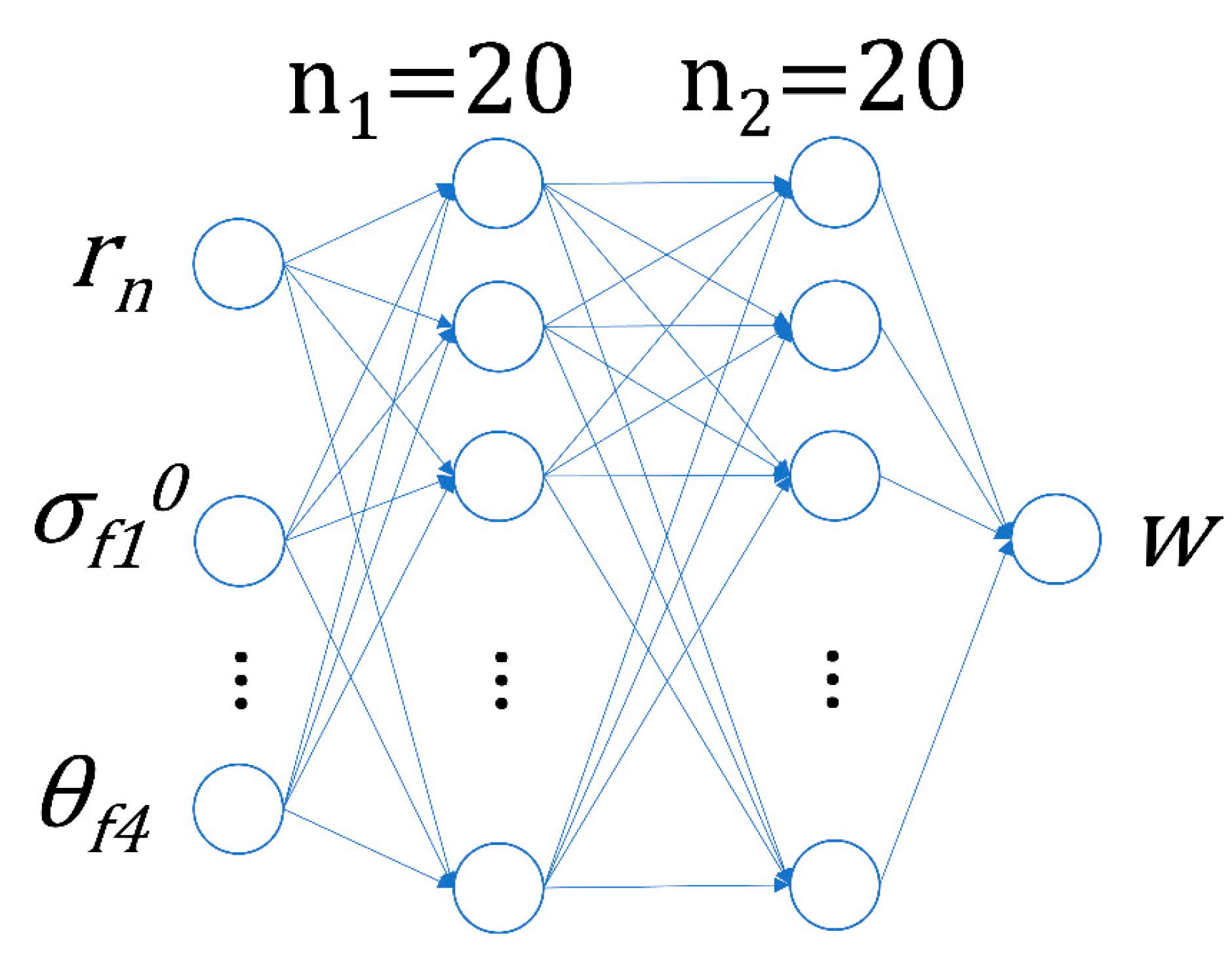
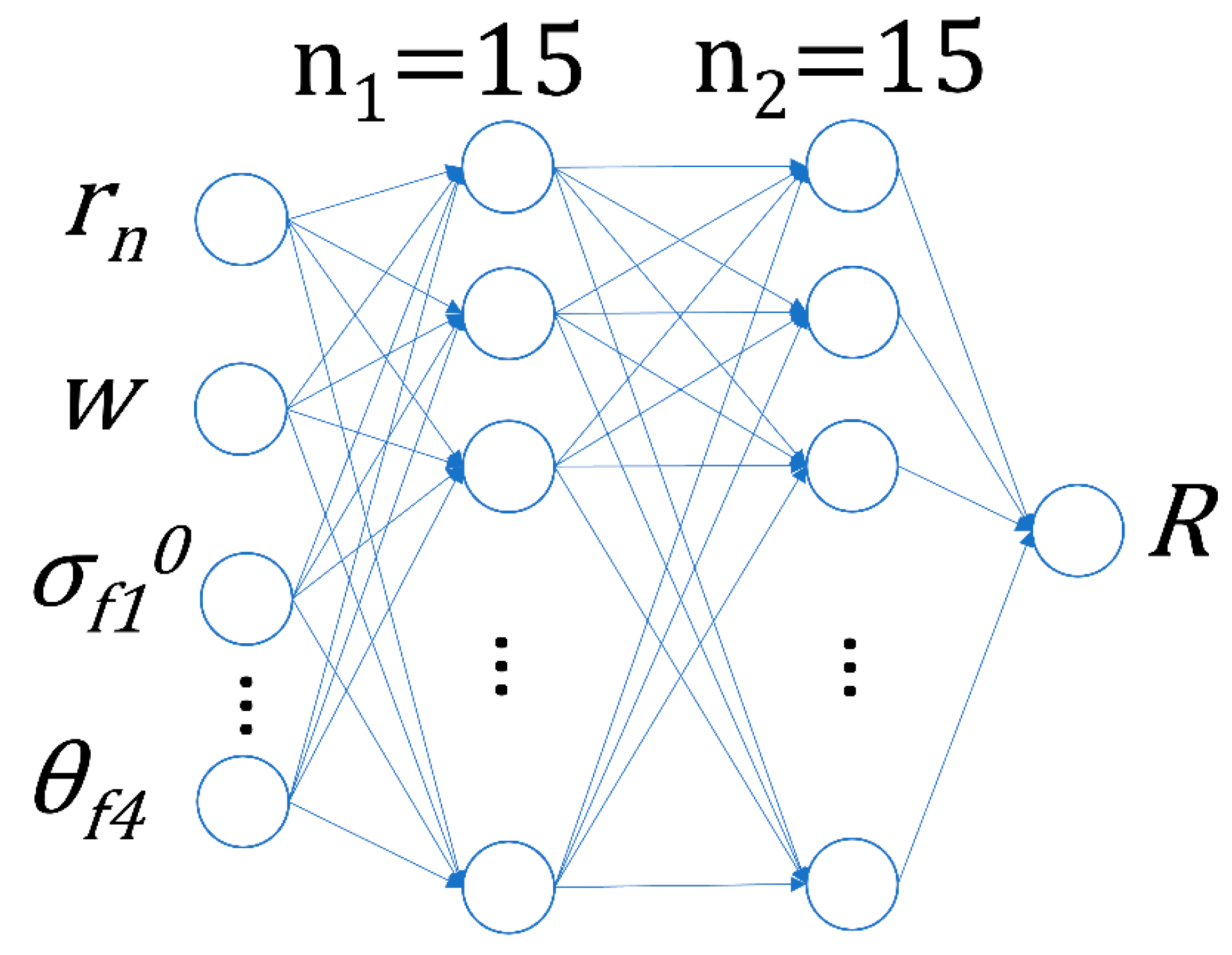
2.4. Neural Network Modeling

The back propagation (BP) neural network is a multilayer feedforward neural network. The main feature of this network is forward signal transmission and backward error propagation. The BP neural network is suitable for solving problems with complex internal mechanisms. The performance of the BP neural network will be affected by the distribution of training samples, neural network structure, neural network activation function and training termination conditions.
Before describing the neural networks used in the study, a brief analysis of the ECMWF and SSM/I data from which the neural networks were constructed and examined is required. Figure 3 shows the data distribution of the ECMWF wind speed and the SSM/I rain rate. The statistical distribution of the data used in constructed and examined is basically the same. Numbers of statistics had to be processed with logarithmic transformation in order to adapt to the big fluctuation in the data. The ECMWF wind speed data are mainly distributed in the low and moderate wind speed section. With the increase in wind speed, the data volume declines sharply. In the range of wind speeds exceeding 30 m/s, only a small amount of the data is matched. It can be seen from the distribution of the SSM/I rain rate (Figure 3d) that the amount of data with no rain or less rain is much larger than that with rain, while the data with high rain rate are far less than that with low rain rate. When the amount of data is not enough, the neural network-based model cannot get the best fitting effect. Thus, the data used for training and testing were those with ECMWF wind speeds less than 30 m/s and SSM/I rain rates less than 20 mm/h.
In neural network training, a key step is to determine the number of hidden layers and neurons. In a neural network, hidden layers are needed when the data are nonlinearly separated. Theoretically, the more hidden layers, the better the fitting ability; however, too many hidden layers can cause overfitting. The number of neurons also affects the performance of neural network training. An insufficient number of neurons will lead to underfitting. On the contrary, too many neurons will cause overfitting. In this study, the optimal number of hidden layers and neurons was obtained through repeated practical training. At the beginning, we trained the neural network with one hidden layer and 10 neurons, then gradually added more layers and neurons to test the output of the network. When the difference between output and reference was the smallest, the model was selected.
In this study, only HY-2A scatterometer measurements and corresponding geometric parameters were used to retrieve the wind speed. Three separate neural network models were constructed: two for wind speed, which are represented by NNW1 and NNW3, and another one for rain rate, which is represented by NNW2 below. The data processing flow in Figure 4 shows the inputs and outputs of different models and the interconnections between them.
NNW1 is used to establish the mapping relationship between HY-2A NRCS, observation geometry and wind speed. The wind speed output from NNW1 is an input for NNW2, which is used to fit a preliminary rain rate. The inputs of NNW3 include the HY-2A dataset and the interim outputs (wind speed and rain rate) from NNW1 and NNW2; the output of NNW3 is the final retrieved wind speed.
It is feasible to use one neural network to improve the wind speed contaminated by rainfall, but better results can be obtained by using three neural networks. The data affected by rainfall account for only about 8% of the total data. Therefore, when training NNW1 and NNW2, we used training samples which expanded the proportion of rainfall-contaminated data to help NNW1 and NNW2 characterize the relationship among HY-2A data, rain rate and wind speed. NNW3 was trained by the data in their original distribution to ensure that the final output wind speed reflects the ‘true’ situation.
Rainfall affects the NRCS, it also affects the wind direction retrieved using scatterometers. The volume scattering of raindrops increases the non-wind information in the backscatter signal, thus weakening the wind speed/direction information in the backscatter coefficient. In addition, the splashing caused by raindrops changes the roughness of the sea surface, which destroys the modulation effect of the relative wind direction on the backscatter coefficient, resulting in the larger deviation of the retrieved wind direction. As a result, it is very difficult to use a simple neural network to eliminate the impact of rainfall on wind direction. Another reason is that the 180° ambiguity of wind direction makes it difficult for the neural network to accurately fit the wind direction. Integrating wind direction into the neural network will increase the complexity of the network. This means that the neural network needs more hidden layers and neurons, which makes the neural network difficult to converge and affects the effect of wind speed fitting. Based on the above reasons, the main objective of this study is to improve the wind speed affected by rainfall, which is easier to do.
When the ECMWF wind speed is larger than 30 m/s and the SSM/I rain rate is larger than 20 mm/h, there are not enough collocated data to train the neural network. Therefore, the ECMWF wind speed used for training and testing is 0.1–30 m/s, and the range of SSM/I rain rate is 0–20 mm/h. The modeling data used in NNW1 and NNW2 network training include the ECMWF wind speed with a sampling interval of 1m/s, the SSM/I rain rate with an interval of 1 mm/h, and the HY-2A WVC column number. Each interval sampled 50 data points. To ensure an even distribution of the input data, a random sampling with replacement strategy was used when the data points in an interval were less than 50. Finally, 555,700 groups of matched data were obtained. The data used for NNW3 network training were randomly extracted from 10% of all training data.
Since the BP neural network uses a gradient descent algorithm, both the inputs and outputs are normalized before training. We initialized the bias with 0 and initialized the weights randomly. The learning step size was set to 0.9, 0.8, …, 0.1, and the maximum number of iterations for each step was 600. The neural network structure for NNW1 is shown in Figure 5. The input layer for the NNW1 model includes nine input terminals, which are the column number of the HY-2A WVC, represented by the symbol rn; the average backscatter coefficients of four different views, represented by the symbol σfN0 (N = 1, 2, …, 4); and the average azimuth angles, represented by the symbol θfN (N = 1, 2, …, 4); each hidden layer includes 20 neural nodes; the output is the ECMWF wind speed, represented by w.
The neural network structure for NNW2 is shown in Figure 6. This network has one input layer, two hidden layers and one output layer. The input layer includes 10 input terminals, which are the column number of the HY-2A WVC, denoted as rn; the ECMWF wind speed, denoted as w; the average backscatter coefficients of four different views, denoted as σfN0; and the average azimuth angles, denoted as θfN (N = 1, 2, …, 4); each hidden layer includes 15 neural nodes; the output is the SSM/I rain rate, denoted as R.
The NNW1 and NNW2 networks were trained to establish the mapping relationship between the HY-2A measurements, geometric parameters and the reference ECMWF wind speed and SSM/I rain rate. However, due to the processing of the sampling strategy, the data distribution is not statistically consistent with the real situation measured using the HY-2A scatterometer. Therefore, a third neural network trained by the data in their original distribution was constructed to ensure that the output wind speed is less affected by the data sampling method. The neural network structure for NNW3 is shown in Figure 7. This neural network includes one input layer, two hidden layers and one output layer. The input layer includes 11 input terminals, which are the column number of the HY-2A WVC, represented by the symbol rn; the average backscatter coefficients of four different views, represented by the symbol σfN0 (N = 1, 2, …, 4); the average azimuth angles, represented by the symbol θfN (N = 1, 2, …, 4); the output of NNW1, represented by w’; and the output of NNW2, represented by R’; each hidden layer includes 15 neural nodes; the output is the ECMWF wind speed, represented by w.

3. Results

In Section 2, the wind field retrieval method was used to verify the wind accuracy of the HY-2A scatterometer under rainy and rain-free conditions. The verification results showed that the wind speed from rain-contaminated HY-2A measurement data was overestimated compared to the ECMWF wind speed. To improve the wind measurement accuracy of the HY-2A scatterometer under the impact of rain, the BP neural network was introduced. In this section, we validate the performance of the neural network model using ECMWF wind speed and TAO buoy wind speed data, as well as TAO linearly corrected ECMWF data.

3.1. Verification of Neural Network-derived Wind Speed Using ECMWF Data

The data used to test the accuracy of the neural network models for wind speed retrieval were the collocated data of the HY-2A backscatter coefficient, ECMWF wind speed, and SSM/I rain rate that were not involved in the training process, with a total of 175,049 data points. The wind speed predicted by the neural network under rainy and rain-free conditions was tested with the ECMWF wind speed, and the error statistics were assessed according to the retrieved wind speed interval of 1 m/s.
The test results are shown in Figure 8. Figure 8a,b present the statistical results of the wind speed bias and the corresponding RMS values under rain-free and rainy conditions, respectively. The blue circles and red asterisks, respectively, represent RMS and bias values between the retrieved wind speed and the ECMWF wind speed (NNW wind speed minus ECMWF wind speed). In Figure 8, it is clear that most biases between the neural network-fitted wind speed and the ECMWF wind speed are less than 1 m/s in each wind speed interval. The mean errors of the wind speed fluctuate close to zero under both rainy and rain-free conditions, indicating that the retrieved HY-2A scatterometer wind speed has no significant systematic deviation under both rainy and rain-free conditions. However, as the wind speed increases, the RMS gradually increases. In the case of high wind speed, there are few data for training and testing, thus, the random error of the wind speed retrieved by the neural network increases.
Figure 9a,b are the scatter plots of the retrieved HY-2A wind speed and the ECMWF wind speed under rain-free and rainy conditions, respectively. Compared with Figure 3, under rainy conditions, most of the data between the retrieved wind speed and the ECMWF wind speed are distributed along the 1:1 line, showing an obvious linear relationship. The degree of dispersion is smaller than that in Figure 3. Comparing with Figure 3b, it can be clearly seen that the HY-2A wind speed fitted using the neural network model is closer to the ECMWF wind speed. At the same time, in Figure 3a, it can be considered that under rain-free conditions, the neural network model can obtain better accuracy than the MLE method.
We also provide the statistical results in the upper left corner of Figure 9a,b. Bias and RMS represent the mean value and root mean square value of the wind speed difference between the retrieved HY-2A wind speed and the ECMWF wind speed under rainy and rain-free conditions. Under rain-free conditions, the bias between the neural network-retrieved wind speed and the ECMWF wind speed is −0.08 m/s with RMS of 1.16 m/s. Compared with the bias and RMS of the wind speed retrieved using the conventional MLE method in Figure 3a, both can reliably retrieve the wind speed under rain-free conditions. In Figure 9b, when the NRCS measured using the HY-2A scatterometer is contaminated by rain, the bias between the retrieved wind speed and the ECMWF wind speed is 0.19 m/s, which is smaller than the bias (1.09 m/s) of the conventional MLE method. The RMS is also reduced to 1.81 m/s, indicating that the neural network model has a better effect on improving the accuracy of the HY-2A scatterometer wind measurement under rainy conditions.
It can be seen that the neural network model provided an improvement in the wind speed under rainy conditions. To further confirm the performance of the neural network model, biases and RMSs between the HY-2A wind speed and the ECMWF wind speed were calculated with a rain rate interval of 1 mm/h and range of 1–20 mm/h, and the statistical results are shown in Figure 10. The blue circles and red asterisks represent the results of the statistical error between MLE-retrieved wind speed and ECMWF wind speed and those between neural network-retrieved wind speed and ECMWF wind speed, respectively. In Figure 10a, the bias statistical results indicate that with the increase in rain rate, the bias for the MLE method also increases, while the bias for the neural network model is relatively stable at less than 1 m/s. Figure 10b shows that in each rain rate interval, the RMS error of wind speed retrieved using the neural network is smaller than that retrieved using the MLE method. The neural network significantly improves the accuracy of HY-2A wind speed measurement under rainfall conditions.
Figure 11 shows the histogram of the difference between the retrieved HY-2A wind speed and the ECMWF wind speed. In the figure, the bias approximately shows a normal distribution, and the data with an error range of −1.5–1.5 m/s account for about 80%, indicating that the difference is not significant. It can be considered that the HY-2A sea surface wind speed retrieved using the neural network is improved with respect to the reference HY-2A winds retrieved using the MLE method.
Figure 12a shows the bias and RMS between all the HY-2A wind speeds retrieved using the neural network and the ECMWF wind speeds for each wind speed interval. In this figure, at moderate wind speeds, the bias in each interval is very small. As can be seen from Figure 12b, when the wind speed is too low or too high, there are fewer data to train and verify the neural network. Therefore, the biases and RMSs for low wind speed (<4.0 m/s) and high wind speed are large. Therefore, the fitted wind speed is lower than 25 m/s. However, the statistical result indicates that the neural network-retrieved wind speed of the HY-2A scatterometer mimics the ECMWF wind speeds to some extent, and it is suitable for both rainy and rain-free conditions.

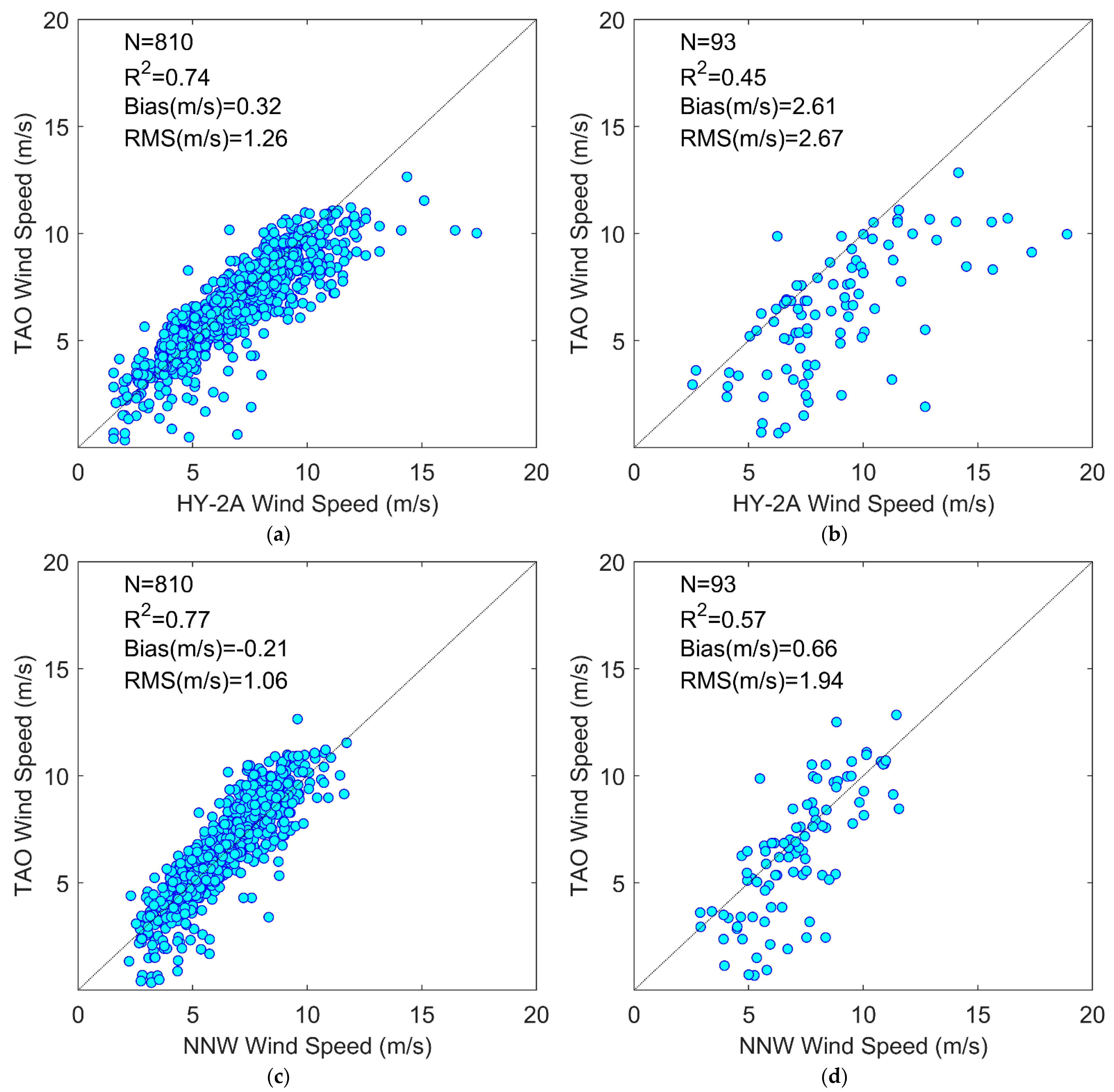
3.2. Verification of Neural Network Wind Speed Using TAO Data

Previously, we used ECMWF data as a reference to verify the accuracy of the wind speed retrieved using the neural network. Next, we use TAO buoy data as a reference to further verify the accuracy of the wind speed retrieved using the neural network. The temporal window and spatial window for matching TAO data and SSM/I data with HY-2A data are set to 10 min and 12.5 km, respectively. SSM/I rain rate data were used for rain flagging, and TAO wind speed was used to verify the wind speed retrieved using the MLE method and the neural network model. HY-2A, TAO and SSM/I data in the entire year of 2013 were matched to construct the dataset for verification. Due to the differences in spatial and temporal distribution among TAO data, SSM/I data and HY-2A data, only 903 data samples were matched. Among 903 data samples, 93 data samples were flagged as rain and 810 data samples were flagged as no rain according to the SSM/I rain rate.
Figure 13 shows scatter plots of wind speed retrieved using different methods and the TAO buoy wind speed and the statistical results are provided in the upper left corner of this figure. N is the number of data points, R2 is the R-square; bias and RMS are the average value and root mean square of the wind speed difference between the retrieved wind speed and the TAO wind speed. The black dashed line is the 1:1 line.
Figure 13a shows the scatter plot between the wind speed retrieved using the MLE method and the TAO wind speed under rain-free conditions, while Figure 13c shows the scatter plot between the wind speed predicted by the neural network and the TAO wind speed under rain-free conditions. Figure 13a,c indicate that both the MLE wind speed and the neural network wind speed are in good agreement with the TAO wind speed and have low dispersion. Statistical results show that the difference between neural network wind speed and TAO wind speed is less than that between MLE wind speed and TAO wind speed.
Figure 13b,d show the scatter plot between MLE-retrieved wind speed and TAO wind speed and the scatter plot between neural network-predicted wind speed and TAO wind speed under rainy conditions, respectively. In Figure 13b, most of the wind speed data pairs are located below the diagonal, indicating that the wind speed retrieved using the MLE method is significantly higher than the TAO wind speed. In contrast, Figure 13d shows that the matched data points of wind speed retrieved using the neural network are basically distributed on both sides of the diagonal line, indicating that the systematic deviation between the wind speed retrieved using the neural network and the wind speed measured using TAO buoy is relatively small. It shows that under rainy conditions, the accuracy of wind speed retrieved using the neural network is better than that retrieved using the MLE method. This result is consistent with the results verified by ECMWF, which indicates that the neural network can improve the sea surface wind speed of scatterometers affected by rainfall.

3.3. Validation with TAO Linear Calibrated ECWMF Data

In the process of training the neural network, we used the ECMWF wind speed data as the modeling data, so it was better to use different data as the validation data. In Section 3.2, we tried to verify the accuracy of the inverted wind speed with the TAO buoy data, but due to the limitation of the data volume of the matched data, the validation data under the rainy condition are fewer. We needed a different kind of data from ECMWF for validation, and to further confirm whether the accuracy of the neural network-inverted wind speed is in accordance with our expectation for it. In this subsection, we use the TAO buoy data as a reference to linearly calibrate the ECMWF data, making them closer to the TAO data. The linear calibration compensates for the problem of wind-speed-bias-dependent manner and insufficient data volume that may exist during the validation process using the ECMWF and TAO data. We used the ECMWF and TAO buoy data for the whole year of 2013 for the matching, and a total of 111,869 data pairs were obtained. Only a very small fraction of the wind speeds measured using the TAO buoys exceeded 15 m/s, and in addition, when the wind speeds were less than 1 m/s, there were fewer data and the measurement errors were random, so we computed the 1–15 m/s wind speed bias as the data for the fitted curves. Figure 14 is a plot of the fitted curves of the bias between ECMWF and TAO. Based on the fitted curves, it is possible to calculate the biases of the ECMWF data for wind speeds in the range of 1–15 m/s. Removing these deviations from the ECMWF wind speeds gives wind speeds closer to the TAO.
In Section 3.1, we use half of the full data for validation while ensuring that there are enough data for training, as more data may cover a wider range of rain rates and wind speed conditions. However, if we use data similar to the distribution of the training data for validation, the validation results will be biased toward the training data, which will affect the ‘real’ validation results. Therefore, we extracted half of the data used in Section 3.1 as the validation data used in this section. The ECMWF wind speeds used in this section were corrected according to the linear calibration method mentioned above, which changes the distribution of the data. Figure 15a,b show the distribution of the original ECMWF wind speeds and the calibrated ECMWF wind speeds, respectively. When the ECMWF wind speed exceeds 15 m/s, there are almost no paired data of TAO wind speed and ECMWF wind speed, and the authenticity of the fitted curves cannot be guaranteed, which affects the effect of deviation removal. Therefore, we set the statistical wind speed distribution range to 1–15 m/s.
Scatter plots of linearly calibrated ECMWF wind speed versus MLE-inverted wind speed and NNW-inverted wind speed, categorized by the presence or absence of precipitation, are shown in Figure 16. The R-squared values, bias between different wind speeds, RMS and number of data points for linear calibration wind speed versus inversion wind speed of the different methods are labeled at the top of each plot. Figure 16a,b show the scatter plots of the MLE-inverted wind speeds versus the reference wind speeds under no rain effect and rain conditions, respectively. The comparison of the scatter in the two plots shows that the agreement between the linearly calibrated ECMWF wind speeds and the MLE wind speeds is better under the no rain condition, while the scatter distribution of the MLE-inverted wind speeds versus the linearly corrected wind speeds is more dispersed under the influence of rain, with an R-squared value of 0.525 and a bias of 0.91 m/s. The validation results show that the difference between the MLE-inverted wind speeds and the linearly corrected wind speeds under no rain conditions is small (there is no dependence on the ECMWF wind speeds in the wind speeds inverted using the MLE method), suggesting that the linearly calibrated ECMWF wind speeds as reference data can illustrate the effectiveness of the NNW-inverted wind speeds to some extent.
Figure 16c,d show the scatter plots of the NNW-inverted wind speeds versus the ECMWF wind speeds without and with rainfall effects, respectively. A comparison of Figure 16a,c shows that the scatter plot distributions of the two are similar, and the R-squared, bias and RMS values are very close to each other. The statistics of the NNW-inverted wind speed is slightly better than that of the MLE method, but the difference between the two is not significant. Comparing Figure 16b,d under the rainfall influence condition, unlike the MLE wind speed which shows obvious deviation, the scatter plots of the NNW inversion wind speed and the linearly calibrated ECMWF wind speed are basically distributed along the diagonal line, which indicates that the agreement between the two is better, and the R-squared value in the statistical results is also 0.754, and the deviation is reduced to 0.22, which supports the smaller difference between the NNW wind speed and the linearly calibrated wind speed under the rainfall influence. The linearly calibrated ECMWF wind speeds are not exactly equivalent to the TAO wind speeds, and the neural network is trained using the ECMWF data, so using the linearly corrected ECMWF wind speed data as the validation data may lead to an increase in the bias between the inverted NNW wind speeds and the reference wind speed.

4. Discussion

Under rainy conditions, the influence of rainfall on the NRCS is the main reason for the overestimation of the retrieved wind speed. When the rain rate becomes very large, the effect of volume scattering on the microwave signal is so large that the scatterometer cannot receive the backscatter signal from the sea surface, and the backscatter coefficient has no information of sea surface wind. Therefore, when using a neural network to improve the scatterometer wind speed affected by rainfall, this situation should be considered and the quality of the scatterometer data should be checked. Figure 10 presents the bias and RMS values of the retrieved wind speed as a function of SSM/I rain rate. The statistical results show that when the rain rate is less than 20 mm/h, the volume scattering effect of raindrops is not large enough to submerge the backscatter signal from the sea surface. As a result, the scatterometer can still capture the wind speed information.
In this study, we used ECMWF ERA5 wind speed and SSM/I rate data as part of the training data for the neural network. Recent studies [13,35] have shown that in the assimilation process of NWP, the influence of moisture flow and downdraft has not been solved, while rainy conditions usually accompany them. ECMWF wind is based on the assimilation data of NWP; thus, the increase in the random error of the wind speed may be due to this reason.
Most of the SSM/I data cannot be completely spatio-temporally collocated with the HY-2A data. Therefore, the difference between the real rainfall situation in the HY-2A footprint and the SSM/I rain rate will cause errors, but these errors do not appear uniform in the case of rain or no rain. We analyzed the collected SSM/I data, and found that the data with rainfall account for only 8% of the total data, and most of the cases are no rain.
Training of neural networks requires a large amount of data. However, the proportion of scatterometer measurement data in the high wind speed segment is relatively small; thus, it is difficult to obtain data under heavy rain conditions. The applicability of the neural network model constructed in this study has some limitations under the conditions of high wind speeds and a high rain rate. Under the condition of high wind speeds or heavy rain, the accuracy of the wind speed retrieved using the neural network decreases. Collecting more data under the conditions of high wind speeds or heavy rain, and adding these data to the training of the neural network is an effective method to improve the accuracy of wind speed retrieved using the neural network. At the same time, we will also try to use more advanced machine learning algorithms to improve the accuracy of wind speed inversion under conditions of high wind speeds and heavy rain in future work. In addition, understanding the coupling relationship between high rainfall and high wind speeds and combining the physical model with the neural network is another direction of improvement worth exploring in depth.
In this study, a new technique to improve the accuracy of the HY-2A wind measurements under rainy conditions without the need for external data was explored by constructing neural network models. We consider this technique as a basis for creating a reprocessed wind speed record, and it has room for further refinement due to the limitations of the data mentioned above and the neural network itself. We expect that in future research we will be able to overcome these limitations and provide an implementable method for obtaining higher quality real-time data for operational scatterometer wind measurements.

5. Conclusions

The Ku-band scatterometers are sensitive to rainfall, which leads to reduced accuracy of wind measurements. In this study, by collocating HY-2A scatterometer data, ECMWF wind field data, and SSM/I rain rate data, BP neural networks were trained and constructed, which can be used to retrieve the wind speed from the HY-2A scatterometer under rainy and rain-free conditions. In this study, the ECMWF wind speed and the SSM/I rain rate were used for modeling. During the inversion, only the scatterometer measurement data and relevant observational parameters are required to retrieve the sea surface wind speed. The main conclusions of our research are as follows:
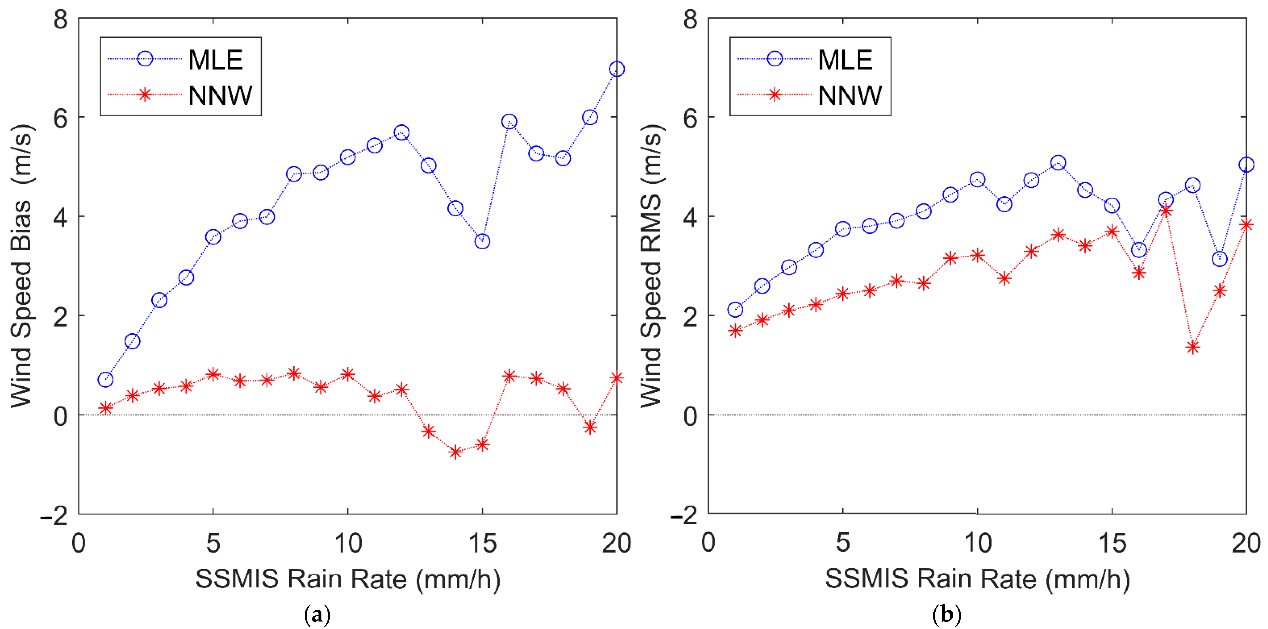
  • The statistical results of the HY-2A wind speed inverted using the conventional MLE method and the ECMWF wind speed show that the HY-2A wind speed has good agreement with the ECMWF wind speed under rain-free conditions. In comparison, the rain-affected HY-2A wind speed is higher than the ECMWF wind speed, indicating that the rain contaminates the scatterometer measurements and introduces errors in the HY-2A wind speed.
  • The BP neural network was used to construct wind speed retrieval models suitable for both rainy and rain-free conditions. In the validation, the ECMWF wind speed, TAO wind speed and ECMWF wind speed with TAO linear correction were used as references. The verification shows that the bias between the wind speed retrieved using the neural network model and the reference wind speed is close to zero. In the case of rain, the bias is slightly higher than that in case of the rain-free conditions. The results indicate that the wind speed retrieved using the neural network is less biased, and the wind measurement accuracy of the HY-2A scatterometer affected by rain is improved.
  • In this study, due to the lack of higher wind speeds and higher rain rate data, the appropriate range for neural network fitting is 0–20 mm/h for the rain rate and 0.1–30 m/s for the wind speed. Scatterometer wind direction retrieval is also affected by rainfall. Correcting the influence of rainfall on wind direction will be one of our next research works.
  • HY-2B and HY-2C are the new operational HY-2 series satellites, and the measurement accuracy of their scatterometers is higher than that of HY-2A. In the future, we will add the data from HY-2B or HY-2C to further explore the methods to improve the wind measurement accuracy of Ku-band scatterometers.

Author Contributions

Conceptualization, X.X.; investigation, methodology, J.W. and X.X.; data curation, software, visualization, writing—original draft, J.W.; Writing—review and editing, project administration and funding acquisition, X.X.; formal analysis, supervision, R.D., X.X., M.L. and X.Y.; validation, M.L. and X.Y. All authors have read and agreed to the published version of the manuscript.

Funding

This work was funded in part by the National Key Research and Development Program of China under Grant 2022YFC3104901, and in part by the National Natural Science Foundation of China under Grant 41876204.

Data Availability Statement

Not applicable.

Acknowledgments

The authors would like to thank the European Centre for Medium-Range Weather Forecasts (ECMWF), the National Data Buoy Center (NDBC), and the Remote Sensing Systems (RSS) for providing the reanalysis wind field data, the TAO buoy data, and the SSM/I radiometer rain rate data, respectively.

Conflicts of Interest

The authors declare no conflict of interest.

Abbreviations

GMFGeophysical model function
WVCWind vector cell
QCQuality control
NRCSNormalized radar cross section
NNWNeural network
MLEMaximum likelihood estimation

References

  1. Liu, W.T. Progress in Scatterometer Application. J. Oceanogr. 2002, 58, 121–136. [Google Scholar] [CrossRef]
  2. Chelton, D.B.; Freilich, M.H. Scatterometer-Based Assessment of 10-m Wind Analyses from the Operational ECMWF and NCEP Numerical Weather Prediction Models. Mon. Weather. Rev. 2005, 133, 409–429. [Google Scholar] [CrossRef]
  3. Weissman, D.E.; Bourassa, M.A.; Tongue, J. Effects of Rain Rate and Wind Magnitude on SeaWinds Scatterometer Wind Speed Errors. J. Atmos. Ocean. Technol. 2002, 19, 738–746. [Google Scholar] [CrossRef]
  4. Draper, D.W.; Long, D.G. Simultaneous wind and rain retrieval using SeaWinds data. EEE Trans. Geosci. Remote. Sens. 2004, 42, 1411–1423. [Google Scholar] [CrossRef]
  5. Weissman, D.E.; Bourassa, M.A. Measurements of the Effect of Rain-Induced Sea Surface Roughness on the QuikSCAT Scatterometer Radar Cross Section. In Proceedings of the IEEE Transactions on Geoscience and Remote Sensing, Barcelona, Spain, 23–28 July 2007. [Google Scholar]
  6. Verhoef, A.; Vogelzang, J.; Stoffelen, A.D. ScatSat-1 Wind Validation Report 25 km (OSI-112-a) and 50 km (OSI-112-b) Wind Products, EUMETSAT Ocean and Sea Ice Satellite Application Facility Document SAF/OSI/CDOP3/KNMI/TEC/RP/324, Version 1.0, KNMI, De Bilt, The Netherlands. 2018. Available online: https://scatterometer.knmi.nl/publications/pdf/osisaf_cdop3_ss3_valrep_scatsat1_winds.pdf (accessed on 26 January 2022).
  7. Xu, X.; Stoffelen, A.; Meirink, J.F. Comparison of Ocean Surface Rain Rates From the Global Precipitation Mission and the Meteosat Second-Generation Satellite for Wind Scatterometer Quality Control. IEEE JSTARS 2020, 13, 2173–2182. [Google Scholar] [CrossRef]
  8. Contreras, R.F.; Plant, W.J.; Keller, W.C.; Hayes, K.; Nystuen, J. Effects of rain on Ku-band backscatter from the ocean. J. Geophys. Res. 2003, 108, 3165. [Google Scholar] [CrossRef]
  9. Portabella, M.; Stoffelen, A. Rain Detection and Quality Control of SeaWinds. J. Atmos. Ocean. Technol. 2001, 18, 1171–1183. [Google Scholar] [CrossRef]
  10. Alpers, W.; Zhang, B.; Mouche, A.; Zeng, K.; Chan, P.W. Rain footprints on C- band synthetic aperture radar images of the ocean–Revisited. Remote Sens. Environ. 2016, 187, 169–185. [Google Scholar] [CrossRef]
  11. Moore, R.; Chaudhry, A.H.; Birrer, I. Errors in Scatterometer–Radiometer Wind Measurement Due to Rain. IEEE J. Ocean. Eng. 1983, 8, 37–49. [Google Scholar] [CrossRef]
  12. Quartly, G.; Srokosz, M.; Guymer, T. Understanding the effects of rain on radar altimeter waveforms. Adv. Space Res. 1998, 22, 1567–1570. [Google Scholar] [CrossRef]
  13. Tournadre, J. Determination of Rain Cell Characteristics from the Analysis of TOPEX Altimeter Echo Waveforms. J. Atmos. Ocean. Technol. 1998, 15, 387–406. [Google Scholar] [CrossRef]
  14. Tournadre, J.; Quilfen, Y. Impact of rain cell on scatterometer data: 1. Theory and modeling. J. Geophys. Res. Atmos. 2003, 108, 3225–3243. [Google Scholar] [CrossRef]
  15. Tournadre, J.; Quilfen, Y. Impact of rain cell on scatterometer data: 2. Correction of Seawinds measured backscatter and wind and rain flagging. J. Geophys. Res. Ocean. 2005, 110, 7023–7039. [Google Scholar] [CrossRef]
  16. Portabella, M.; Stoffelen, A.; Lin, W.; Turiel, A.; Verhoef, A.; Verspeek, J.; Poy, J. Rain Effects on ASCAT-Retrieved Winds: Toward an Improved Quality Control. IEEE Trans. Geosci. Remote Sens. 2012, 50, 2495–2506. [Google Scholar] [CrossRef]
  17. Xu, X.; Stoffelen, A. Improved Rain Screening for Ku-Band Wind Scatterometry. IEEE Trans. Geosci. Remote Sens. 2020, 58, 2494–2503. [Google Scholar] [CrossRef]
  18. Huddleston, J.; Stiles, B. A multidimensional histogram rain-flagging technique for SeaWinds on QuikSCAT. In Proceedings of the 2000 IEEE International Geoscience and Remote Sensing Symposium, Honolulu, HI, USA, 24–28 July 2000. [Google Scholar]
  19. Ahmad, K.; Jones, W.; Kasparis, T. Oceanic Rainfall Retrievals using passive and active measurements from SeaWinds Remote Sensor. In Proceedings of the 2007 IEEE International Geoscience and Remote Sensing Symposium, Barcelona, Spain, 23–27 July 2007. [Google Scholar]
  20. Moore, R.; Braaten, D.; Natarajakumar, B.; Kurisunkal, V.J. Correcting scatterometer ocean measurements for rain effects using radiometer data: Application to SeaWinds on ADEOS-2. In Proceedings of the 2003 IEEE International Geoscience and Remote Sensing Symposium, Toulouse, France, 21–25 July 2003. [Google Scholar]
  21. Hilburn, K.; Wentz, F.; Smith, D.; Ashcroft, P. Correcting active scatterometer data for the effects of rain using passive mi-crowave data. J. Appl. Meteorol. Clim. 2006, 45, 382–398. [Google Scholar] [CrossRef]
  22. Draper, D.; Long, D. Evaluating the effect of rain on SeaWinds scatterometer measurements. J. Geophys. Res 2004, 109. [Google Scholar] [CrossRef]
  23. Stiles, B.; Yueh, S. Impact of rain on spaceborne Ku-band wind scatterometer data. IEEE Trans. Geosci. Remote Sens. 2002, 40, 1973–1983. [Google Scholar] [CrossRef]
  24. Stiles, B.; Dunbar, R. A Neural Network Technique for Improving the Accuracy of Scatterometer Winds in Rainy Conditions. IEEE Trans. Geosci. Remote Sens. 2010, 48, 3114–3122. [Google Scholar] [CrossRef]
  25. Verhoef, A.; Vogelzang, J.; Verspeek, J.; Stoffelen, A. AWDP User Manual and Reference Guide, NWPSAF-KN-UD-005, version 2.0; EU-METSAT: Darmstadt, Germany, 2010. [Google Scholar]
  26. Lin, W.; Portabella, M.; Stoffelen, A.; Turiel, A.; Verhoef, A. Rain Identification in ASCAT Winds Using Singularity Analysis. IEEE Geosci. Remote Sens. Lett. 2014, 11, 1519–1523. [Google Scholar] [CrossRef]
  27. Stoffelen, A.; Anderson, D. Scatterometer data interpretation: Measurement space and inversion. J. Atmos. Ocean. Technol 1997, 14, 1298–1313. [Google Scholar] [CrossRef]
  28. Figa, J.; Stoffelen, A. On the assimilation of Ku-band scatterometer winds for weather analysis and forecasting. IEEE Trans. Geosci. Remote Sens. 2000, 38, 1893–1902. [Google Scholar] [CrossRef]
  29. Wang, Z.X.; Stoffelen, A.; Zhang, B.; He, Y.J.; Lin, W.M.; Li, X.Z. Inconsistencies in scatterometer wind products based on ASCAT and OSCAT-2 collocations. Remote Sens. Environ. 2019, 225, 207–216. [Google Scholar] [CrossRef]
  30. Verhoef, A.; Vogelzang, J.; Verspeek, J.; Stoffelen, A. PenWP User Manual and Reference Guide, EUMETSAT NWP Satellite Application Facility Document NWPSAF-KN-UD-009, Version 2.2, KNMI, De Bilt, The Netherlands. 2018. Available online: https://nwpsaf.eumetsat.int/site/download/documentation/scatterometer/penwp/NWPSAF-KN-UD009_PenWP_User_Guide_v2.2.pdf (accessed on 10 October 2021).
  31. Badran, F.; Thiria, S.; Crepon, M. Wind ambiguity removal by the use of neural network techniques. J. Geophys. Res. Ocean. 1991, 96, 20521–20529. [Google Scholar] [CrossRef]
  32. Reichstein, M.; Camps-Valls, G.; Stevens, B. Deep learning and process understanding for data-driven Earth system science. Nature 2019, 566, 195–204. [Google Scholar] [CrossRef]
  33. Mejia, C.; Thiria, S.; Tran, N.; Crépon, M.; Badran, F. Determination of the geophysical model function of the ERS-1 scat-terometer by the use of neural networks. J. Geophys. Res 1998, 103, 12853–12868. [Google Scholar] [CrossRef]
  34. Jones, W.L.; Park, J.D.; Donnelly, W.J.; Carswell, J.R.; Mclntosh, R.E.; Zec, J.; Yueh, S. An improved NASA Scatterometer ge-ophysical model function for tropical cyclones. In Proceedings of the 1998 IEEE International Geoscience and Remote Sensing. Symposium Proceedings, Seattle, WA, USA, 6–10 July 1998. [Google Scholar] [CrossRef]
  35. Richaume, P.; Badran, F.; Crepon, M.; Mejía, C.; Roquet, H.; Thiria, S. Neural network wind retrieval from ERS-1 scatterometer data. J. Geophys. Res 2000, 105, 8737–8751. [Google Scholar] [CrossRef]
  36. Lin, M.S.; Song, X.X.; Jiang, X.W. Neural network wind retrieval from ERS-1/2 scatterometer data. Acta Oceanol. Sin.-Engl. Ed. 2006, 25, 35–39. [Google Scholar]
  37. Xu, X.; Stoffelen, A. Wind Retrieval for Cfoscat Edge and Nadir Observations Based on Neural Networks and Improved Principle Component Analysis. In Proceedings of the IGARSS 2019—2019 IEEE International Geoscience and Remote Sensing Symposium, Yokohama, Japan, 28 July–2 August 2019. [Google Scholar] [CrossRef]
  38. Xie, X.T.; Wang, J.; Lin, M.S. A Neural Network-Based Rain Effect Correction Method for HY-2A Scatterometer Backscatter Measurements. Remote Sens. 2020, 12, 1648. [Google Scholar] [CrossRef]
  39. Rivas, M.B.; Stoffelen, A. Characterizing ERA-Interim and ERA5 surface wind biases using ASCAT. Ocean Sci 2019, 15, 831–852. [Google Scholar] [CrossRef]
  40. Thomas, B.R.; Kent, E.C.; Swail, V.R. Methods to homogenize wind speeds from ships and buoys. Int. J. Climatol. 2005, 25, 979–995. [Google Scholar] [CrossRef]
  41. Fang, P.; Zhao, B.; Zeng, Z.; Yu, H.; Lei, X.; Tan, J. Effects of wind direction on variations in friction velocity with wind speed under conditions of strong onshore wind. J. Geophys. Res. Atmos. 2018, 123, 7340–7353. [Google Scholar] [CrossRef]
  42. Bentamy, A.; Croize-Fillon, D.; Perigaud, C. Characterization of ASCAT measurements based on buoy and QuikSCAT wind vector observations. Ocean Sci. 2008, 4, 265–274. [Google Scholar] [CrossRef]
  43. Picaut, J.; Hackert, E.; Busalacchi, A.J.; Murtugudde, R.; Lagerloef, G.S.E. Mechanisms of the 1997–1998 El Niño–La Niña, as inferred from space-based observations. J. Geophys. Res. 2002, 107, 5-1–5-18. [Google Scholar] [CrossRef]
  44. Zou, J.; Xie, X.; Yi, Z.; Lin, M. Wind Retrieval Processing for HY-2A Microwave Scatterometer. In Proceedings of the 2014 IEEE International Geo-science and Remote Sensing Symposium, Quebec City, QC, Canada, 13–18 July 2014. [Google Scholar]
  45. Freilich, M.H. SeaWinds Algorithm Theoretical Basis Document. NASA JPL, Los Angeles, CA, USA, Tech. Rep. NASA ATBD-SWS-01. 1999. Available online: https://ntrs.nasa.gov/api/citations/20160003317/downloads/20160003317.pdf (accessed on 19 May 2022).
  46. Hersbach, H.; Stoffelen, A.; Haan, S. An improved C-band scatterometer ocean geophysical model function: CMOD5. J. Geophys. Res. Ocean. 2007, 112, 3006–3024. [Google Scholar] [CrossRef]
  47. Wentz, F.J.; Smith, D.K. A model function for the ocean-normalized radar cross section at 14 GHz derived from NSCAT ob-servations. J. Geophys. Res 1999, 104, 11499–11514. [Google Scholar] [CrossRef]
  48. Stoffelen, A.; Verspeek, J.; Vogelzang, J.; Verhoef, A. The CMOD7 geophysical model function for ASCAT and ERS wind retrievals. IEEE J. Sel. Top. Appl. Earth Obs. Remote Sens. 2017, 10, 2123–2134. [Google Scholar] [CrossRef]
  49. Lin, W.; Portabella, M.; Stoffelen, A.; Verhoef, A.; Wang, Z. Validation of the NSCAT-5 Geophysical Model Function for Scatsat-1 Wind Scatterometer. In Proceedings of the 2018 IEEE International Geoscience and Remote Sensing Symposium, Valencia, Spain, 22–27 July 2018. [Google Scholar]
  50. Portabella, M.; Stoffelen, A. A probabilistic approach for SeaWinds data assimilation. Q. J. Roy. Meteor. Soc 2004, 130, 127–152. [Google Scholar] [CrossRef]
Figure 1. Scatter plots and box plots of ECMWF and TAO paired data. (a) Scatter plot of wind speed in rain-free conditions. (b) Box plot of wind direction in rain-free conditions. (c) Scatter plot of wind speed in rainy conditions. (d) Box plot of wind direction in rainy conditions. The dashed line in this figure is the 1:1 line.
Remotesensing 15 04357 g001
Figure 2. Comparisons of retrieved wind speed data from HY-2A and ECMWF under rain-free conditions (a) and rainy conditions (b). The dashed line in these figures is the 1:1 line.
Remotesensing 15 04357 g002
Figure 3. Histogram of ECMWF wind speed and SSM/I rain rate for model training and testing. (a) ECMWF wind speed for model training; (b) ECMWF wind speed for model testing; (c) SSM/I rain rate for model training; (d) SSM/I rain rate for model testing.
Remotesensing 15 04357 g003
Figure 4. Data flow diagram of wind speed retrieval with neural networks.
Remotesensing 15 04357 g004
Figure 5. Schematic diagram of NNW1 neural network topology.
Remotesensing 15 04357 g005
Figure 6. Schematic diagram of NNW2 neural network topology.
Remotesensing 15 04357 g006
Figure 7. Schematic diagram of NNW3 neural network topology.
Remotesensing 15 04357 g007
Figure 8. RMS and bias of wind speed as a function of wind speed. (a) The result of error verification under rain-free conditions, (b) the result of error verification under rainy conditions. The dashed line in the figure indicates that the wind speed bias is 0.
Remotesensing 15 04357 g008
Figure 9. Comparisons of the neural network retrieved HY-2A wind speed and ECMWF wind speed data under rain-free (a) and rainy (b) conditions. The dashed line in the figure represents the 1:1 line.
Remotesensing 15 04357 g009
Figure 10. RMS and bias of wind speed as a function of SSM/I rain rate. (a) The variation curve of wind speed bias versus the SSM/I rain rate, (b) the variation curve of wind speed RMS versus the SSM/I rain rate. The dashed line in the figure indicates that the wind speed bias and RMS is 0.
Remotesensing 15 04357 g010
Figure 11. The wind speed bias histogram.
Remotesensing 15 04357 g011
Figure 12. Dependence of wind speed RMS and bias on the neural network-retrieved wind speed and the wind speed histogram. (a) The result of error verification, the dashed line in the figure indicates that the wind speed bias is 0. (b) The wind speed histogram.
Remotesensing 15 04357 g012
Figure 13. Scatter plots of wind speed retrieved using the MLE method and the neural network with TAO paired data. (a) Scatter plots of MLE wind speed in rain-free conditions. (b) Scatter plots of MLE wind speed in rainy conditions. (c) Scatter plots of NNW wind speed in rain-free conditions. (d) Scatter plots of NNW wind speed in rainy conditions. The dashed line in this figure is the diagonal line.
Remotesensing 15 04357 g013
Figure 14. Fitted curves of the bias between ECMWF and TAO. The blue asterisks in the plot indicate the bias between the ECMWF and TAO wind speeds, and the solid red line indicates the fitted curve.
Remotesensing 15 04357 g014
Figure 15. Histogram of ECMWF wind speed without and with TAO linear calibration. (a) Original ECMWF wind speed; (b) linear calibration ECMWF wind speed.
Remotesensing 15 04357 g015
Figure 16. Scatter plots of wind speed retrieved using the MLE method and the neural network with TAO linearly calibrated ECMWF data. (a) Scatter plots of MLE wind speed in rain-free conditions. (b) Scatter plots of MLE wind speed in rainy conditions. (c) Scatter plots of NNW wind speed in rain-free conditions. (d) Scatter plots of NNW wind speed in rainy conditions. The dashed line in this figure is the diagonal line.
Remotesensing 15 04357 g016
Disclaimer/Publisher’s Note: The statements, opinions and data contained in all publications are solely those of the individual author(s) and contributor(s) and not of MDPI and/or the editor(s). MDPI and/or the editor(s) disclaim responsibility for any injury to people or property resulting from any ideas, methods, instructions or products referred to in the content.

