Abstract
Antarctic mapping with satellite images is an important basic task for polar environmental monitoring. Since the first Chinese marine satellite was launched in 2002, China has formed three series of more than 10 marine satellites in orbit. As global operational monitoring satellites of ocean color series, HY-1C and HY-1D have good coverage characteristics and imaging performance in polar regions, and they provide an effective tool for Antarctic monitoring and mapping. In this paper, Antarctic images acquired by the HY-1 satellite Coastal Zone Imager (CZI) sensor were used to study color matching in the mosaic process. According to the CZI characteristics for Antarctic imaging, experiments were carried out on the illuminance nonuniformity of a single image and color registration of multiple images. A gray-level segmentation color-matching method is proposed to solve the problem of image overstretching in the Antarctic image color-matching process. The results and statistical analysis show that the proposed method can effectively eliminate the color deviation between HY-1 Antarctic images, and the mosaic results have a good effect.
1. Introduction
Antarctica is an important driver of global climate change and the last unexplored continent. Due to bad weather conditions, it is difficult to investigate Antarctica using field observation methods. The development of satellite remote sensing technology has greatly reduced the impact of adverse natural environmental conditions, making monitoring Antarctica rapid and convenient. A satellite remote sensing imagery mosaic map of Antarctica can be used to study the changes in large-scale environmental characteristics, such as glacier mass balance monitoring, ice shelf calving, and Antarctic ecology, to help people better understand the impact of polar changes on global climate change. Relative radiometric normalization (RRN) can be defined as the procedure of adjusting radiometric (or color) distortions from gray levels of a multispectral subject image based on a multispectral reference image [1]. Since multiple images in a mosaic dataset may be captured by multiple sensors, under different illumination conditions or from different seasons, the color statistics inside a single image or between images are inconsistent, which restricts their usage [2]. Therefore, it is necessary to perform RRN processing before image mosaicking.
Since the first Chinese ocean satellite was launched in 2002, China has worked to establish a global operational ocean satellite observation system. Currently, the observation system consists of 10 satellites, which include three series: ocean color series satellites (HY-1), ocean dynamic environment series satellites (HY-2), and ocean surveillance and monitoring series satellites (HY-3) [3]. In this study, Antarctic images obtained from the HY-1C and HY-1D satellites are used to study a color-matching method during the mosaic process. The HY-1C and HY-1D satellites (Table 1) were launched in 2018 and 2020, respectively. They are an operational satellite constellation that belongs to Chinese ocean color satellites. The Coastal Zone Imager (CZI) instrument on board the ocean color series satellites is an optical remote sensing payload. The band includes blue, green, red, and near-infrared channels, with a spatial resolution of 50 m and a swath of 900 km. It can be used to monitor the coastal zone environment, sea ice, red tide, green tide, and marine and polar environments. The large coverage characteristics and good imaging performance of the CZI provide an effective observation method for the Antarctic region.

Table 1.
HY-1C/D satellite introduction.
Mapping with satellite images is important basic work for investigation and research in the Antarctic region. At present, some research institutions have carried out mosaic mapping of Antarctica with satellite images and released data products, and some applications based on these data products have been studied. For example, in 1997, the Byrd Polar and Climate Research Center of the Ohio State University and the Canadian Space Agency (CSA) obtained the Radarsat-1 Antarctic mosaic map with a resolution of 25 m for the first time (the data imaging time was from September to October in 1997) [4]. This work was the first stage of the Radarsat-1 Antarctic Mapping Project (RAMP), and the second stage of the RAMP data was collected from September to November in 2000 [5]. Jezek used RAMP data to discuss changes in several ice shelves and ice sheet margins around Antarctica [6]. In 2007, the United States Geological Survey (USGS), the National Science Foundation, the National Aeronautics and Space Administration (NASA), and the British Antarctic Survey (BAS) jointly produced the Landsat Antarctic Image Mosaic (LIMA) from 1065 Landsat images covering Antarctica between 1999 and 2003 [7,8]. The National Snow and Ice Data Center of the United States developed an Antarctica mosaic image map with a resolution of 250 m based on 260 MODIS images acquired between 2003 and 2004. The Antarctic coastline, ground line, mainly ice shelf coverage, and blue ice distribution were developed based on this MODIS mosaic product [9]. Hui Fengming et al. used Landsat data to conduct mosaic mapping of Antarctic images [10], and the blue-ice areas and their geographical distribution in Antarctica were mapped using the Landsat data associated with the snow grain-size image of the MODIS-Based Mosaic of Antarctica (MOA) dataset [11]. In addition, numerous studies have been conducted to map Antarctica using satellite imagery. Schwaller et al. used Landsat data to study distribution maps of Adelie penguin colonies in Antarctica [12]. Campbell et al. [13] and Scambos et al. [14] used satellite thermal infrared mapping to discover the ultracold surface of East Antarctica, the coldest place on earth. Qiang et al. mapped the ice velocity in Antarctica from Landsat 8 images and InSAR, and revealed mass loss in Wilkes Land, East Antarctica [15].
Image mosaicking is a technique to seamlessly fuse multiple images with overlapping areas into a single composite image [2]. Image registration is an underlying requirement for a successful mosaic. On the one hand, for images without geographic reference information, the purpose of image registration and stitching can be achieved by finding the feature information on the image [16,17], and then establishing a model based on the feature information [18]. On the other hand, for images with geographic reference information, image registration can be directly based on geographic information. In general, geographic registration is mostly used for satellite imagery. Satellite image mosaicking usually consists of five aspects: image registration, extraction of overlapping areas, radiometric normalization (also called radiometric balancing, color adjustment, or color consistency matching), seamline detection, and image blending [19]. Color consistency matching between different images is an important process during image mosaicking, and the main purpose of this process is to eliminate the color differences between mosaic images and make the color consistent. In this paper, we study the color consistency matching method using the HY-1C/D images from Antarctica.
Generally, the image color consistency matching process includes single-image illumination homogenization processing and multi-image color consistency processing [20]. Li et al. used HY-1C data to study a color consistency processing method between images of Antarctica [21]. Image illumination homogenization processing is mainly used to solve the problem of uneven light inside the image, especially for remote sensing images with large swaths. Uneven light correction methods include illumination uniform methods based on additive models, such as the background fitting method and MASK method [22,23], and multiplicative models for illumination uniform methods, such as the homomorphic filtering method [24] and retinex method [25,26]. Yu Xiaobo et al. [27] made a comparative analysis from the different illumination uniform experimental results to address image processing quality and algorithm execution efficiency. The results show that the MASK algorithm has the best illumination uniform effect.
Color consistency processing is used to solve the problem of the color difference among multiple images, and general methods include the histogram matching method, mathematical model method, and mean variance method. A histogram matching method adjusts the histogram of the image according to a specified shape so that it has an approximate shape with the target image and achieves the goal of color consistency. Helmer et al. [28] used the histogram features of overlapping image regions to establish mapping relationships and then processed the image gray level to match the color of the target image. Zhang Qiao et al. [29] optimized the mapping rules during histogram matching, which enriched the image gray level. Xie et al. [30] proposed a guided initial solution of the histogram extreme point matching algorithm to address the global consistency optimization. A mathematical model method mainly statisticizes the pixel features of overlapping areas between images and then fits a linear [31,32] or nonlinear [33,34,35] relationship between the image to be corrected and the target image; thus, image color consistency correction is carried out. Li et al. [2] proposed a pairwise gamma model to coarsely align the color tone between the source and reference images. Then the multiview color alignment is minimized by the least squares adjustment method. Li et al. [36] proposed a series of local linear model approaches and a specific global cost function that can correct global and local color discrepancies simultaneously and preserve image gradient as much as possible. Chen et al. [37] proposed pseudo-invariant feature-based algorithms with polygon features through single-band and multiple-band regression, and applied them to radiometric normalization between Sentinel-2A and Landsat-8 OLI images. The effectiveness of the proposed algorithm is demonstrated by comparing the results with the histogram matching method. A mean variance method, such as the Wallis transform, converts the mean value and variance of an image to be processed into the mean value and variance of the target image through a mathematical relationship to achieve color matching. Based on Wallis, Pan Jun et al. [38] proposed a color balance method that considers both the whole and part of the image, which reduces the dependence of color balance processing on the effect of uniform light processing. Han Yutao [39] studied the problem of grayscale loss after Wallis transformation and verified the effectiveness of the color consistency method. Li Shuo [20] proposed a block weighted Wallis image color consistency processing method to solve the color and contrast differences between images.
Different from the method that fits the pixel-to-pixel features of overlapping region images as previously mentioned, histogram matching is a distribution-based color consistency matching method [19,40]. It can avoid subjectivity in the selection of pseudo point features and image misregistration [37]. The focus of this algorithm is on the digital number (DN) distribution between the subject image and the target image, which is closely linked to the type of terrain objects on the image. Therefore, when using histogram matching methods for color correction, it is necessary to consider the distribution of surface-truth objects on the image. Antarctica is surrounded by ocean and covered by ice and snow year-round. It has a large contrast and dynamic range in optical satellite images. The simplicity of terrain objects on the Antarctic continent is a great guarantee for the applicability of the algorithm. However, if there is a large difference between the types of terrain objects in the subject and reference images, for example, if the subject image includes seawater and glaciers, while the reference image only contains glaciers, the histogram matching results are often poor.
Based on digital image processing and histogram specification theory, data from the CZI instrument on board the HY-1C/D satellites were used to study an image mosaicking color consistency processing method in the Antarctic region. Single-image illumination homogenization processing and multi-image color consistency processing were studied. In the experiment, a color segmentation matching method based on a threshold value is proposed to achieve color consistency between adjacent images and achieve a good effect. In the second chapter, satellite data information, data preprocessing, and image color-matching methods are introduced. In Section 3, the results of nonuniformity correction and image color matching are introduced. In Section 4, the quality of mosaic images is analyzed qualitatively and quantitatively, and the problem of overstretching in color matching is discussed. The full text is summarized in Section 5.
2. Data and Methods
2.1. Data and Preprocessing
The Antarctic images studied in the paper were obtained using the CZI on board the Chinese HY-1C and HY-1D satellites. The data cover the near-infrared (0.76–0.89 μm), red (0.61–0.69 μm), green (0.52–0.60 μm), and blue (0.42–0.50 μm) bands; the spatial resolution is 50 m; and the swath is 900 km. The data product has an L1C processing level, is stored in 32 bit floating-point GeoTIFF format, and is projected in polar stereographic projection over the Antarctic region after radiometric and geometric correction. Four CZI scene datasets were selected (Table 2), and the imaging dates were 3 December 2021, 6 December 2021, 8 December 2021, and 13 December 2021. The data range covers Victoria Land, the Ross Ice Shelf, and the Transantarctic Mountains in Antarctica. There are abundant topographic and geomorphic features in this region, including mountains, glaciers, ice shelves, bare rocks, blue ice, and oceans.
Table 2.
HY-1/CZI datasets used in our experiments.
To reduce the data processing amount for subsequent research, channels 3 (red), 2 (green), and 1 (blue) were selected, and the data type was converted to 8-bit. Then, the data were combined into a true-color RGB image. During satellite acquisition of polar images, because of the sun altitude angle and terrain changes, sometimes, a small amount of abnormally large gray values exist in a few images. To make a better visual effect of the image during the data-type conversion process, a cumulative histogram is introduced into the conversion method to set the extreme value of the image stretch. The maximum intercept frequency is set to , and the pixel value pix() corresponding to frequency in the cumulative histogram is the maximum stretch value in the entire image. A pixel value larger than pix() was set to 255 because pixels with an image value of less than pix() are converted to 0–255 using linear stretching according to the minimum image value and the range between pix(). The conversion procedure is as follows:
where is the L1C product pixel value, is the converted integer data, and is the converted 8-bit value.
2.2. Image Nonuniformity and Correction
Due to the influence of some imaging conditions, such as illumination conditions, sensor performance, clouds, and other factors, some HY-1C/D satellite images in the Antarctic region exhibit nonuniformity. Figure 1 shows an example of the nonuniform luminance phenomenon on Antarctica, which causes great difficulties for the subsequent image mosaic and color consistency process. Therefore, it is necessary to correct the nonuniformity luminance of the single-field image first.
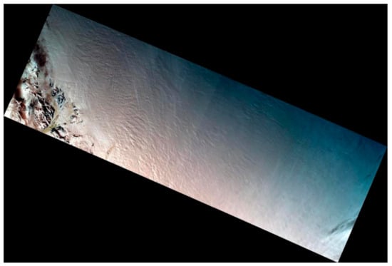
Figure 1.
HY-1/CZI example image of Antarctica (nonuniformity luminance phenomenon).
At present, a commonly used algorithm to correct nonuniformity images is based on the MASK principle. The image luminance distribution can be better simulated using this algorithm. The luminance distribution is used as the background image, which is subtracted from the original image. Then, an artificial light source is added, and a relatively ideal uniform light result can be obtained [41]. However, when using this method, for areas with great contrast in the original image (such as the coastal zone), different background simulation filters or different stretching modes may cause inconsistent stretching effects between the darker (seawater) area and the brighter (ice sheet) area, resulting in obvious luminance differences between the coastline land area and the inland area. To eliminate this effect, the nonuniformity luminance correction method proposed by Li et al. [21] is adopted in this study. In this method, a Gaussian filter with an auxiliary mask is introduced to separate the nonuniform illumination information (feature map) from the image to effectively eliminate this effect. The auxiliary mask can be obtained by a simple threshold method, which mainly identifies the image as a light and dark target (e.g., glacier and seawater). Based on MASK theory, image nonuniformity luminance correction includes the following four steps: (1) luminance feature image extraction, (2) uneven luminance removal, (3) calculation of artificial light sources, and (4) information integration to generate a uniform light image.
2.3. Multi-Image Color Match
The features in the Antarctic satellite images are relatively simple compared with the surface features at the lower latitudes of the earth, and the reflectance of ground object features varies greatly (such as oceans and ice/snow). If an improper method is used in the process of color stretching in an Antarctic image, it is easy to cause excessive stretching and color distortion of some ground object features. Based on histogram specification theory, this study adopts different mapping methods for low-reflectance and high-reflectance features in the process of histogram mapping between the original image and reference image. Meanwhile, to prevent gray-level discontinuity in the image mapping, gray-level linear stretch transformation is used in the mapping rule.
Assume that T (T ∈ [0, 255]) is the threshold of low-reflection objects and high-reflection objects in an Antarctic satellite image, and R(x,y) and O(x,y) are the reference image and the original image, respectively. Then, histogram equalization transformation is performed for the original image and the reference image:
where represent the cumulative histogram transformation of the images R(x,y) and O(x,y), respectively, and and are the histogram equalized results of the reference image and the original image, respectively. According to the mapping rule of minimum , after histogram equalization conversion, assume that the conversion value of the original image O(x,y) gray value range ) is , and the conversion value of the reference image R(x,y) gray value range ) is , and the |−| is the smallest. Then the gray value of the output image is mapped as
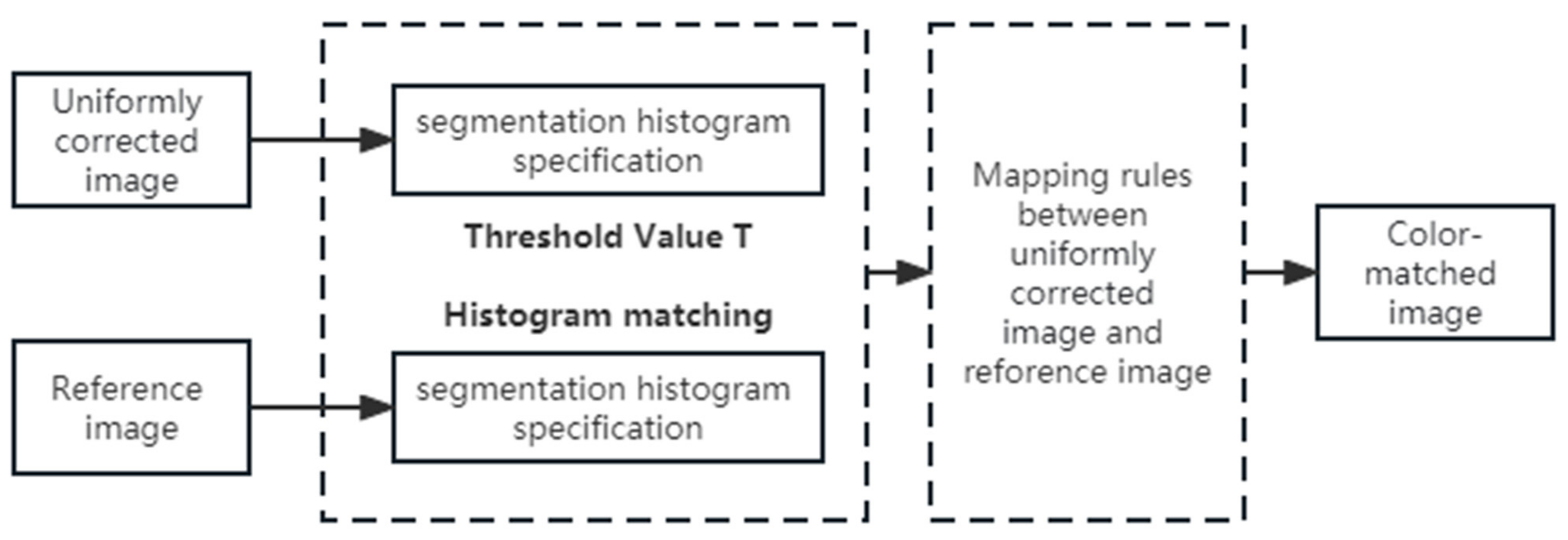
The mapping value I for the gray level M of the original image O(x,y) can be calculated using the above mapping rule, and the gray level of the original image can be converted according to this formula to achieve color correction. The workflow of multi-image color matching processing is shown in Figure 2.
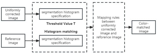
Figure 2.
Multi-image color matching processing.
2.4. Image Color-Matching Process
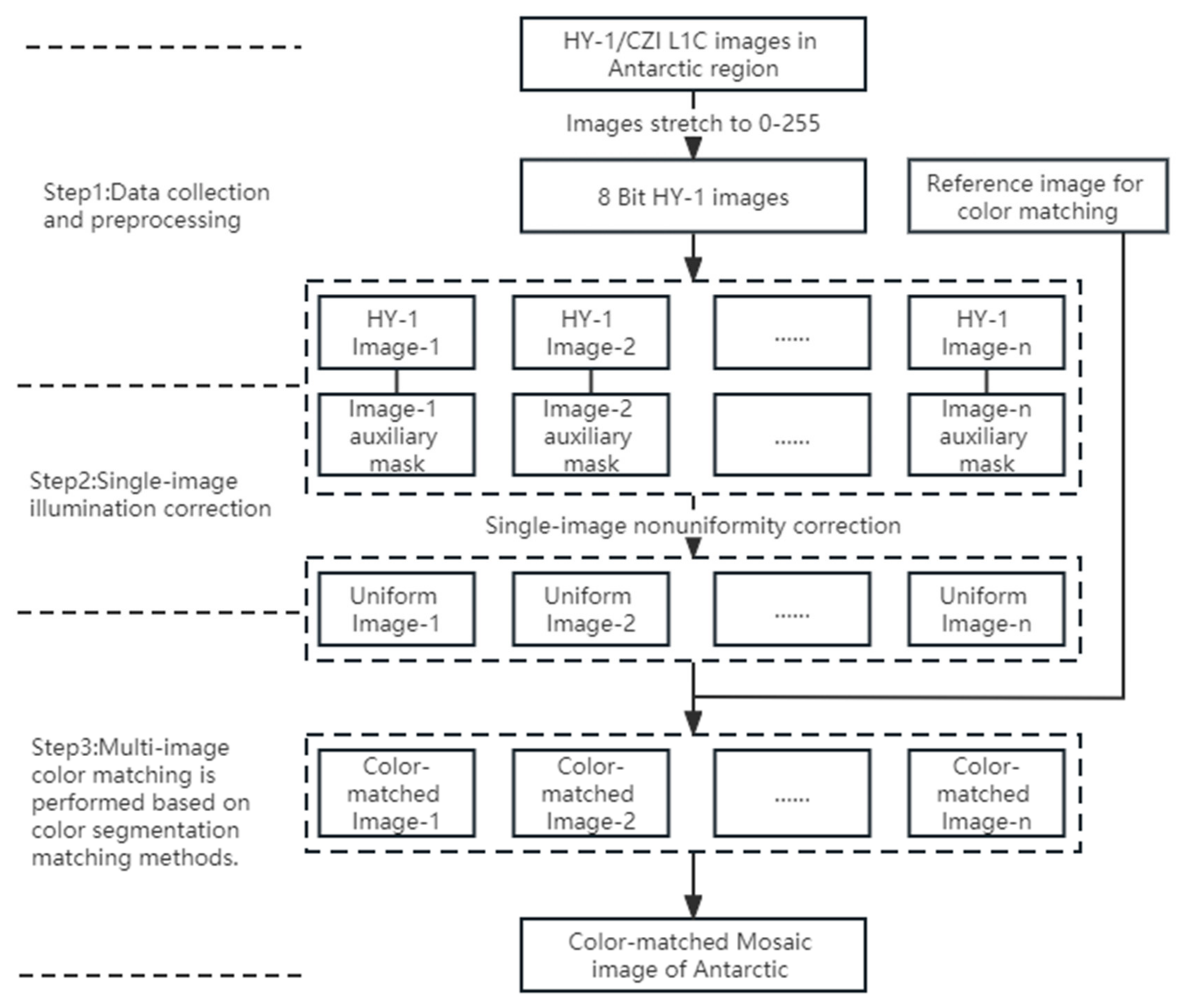
The study of color matching in this paper consists of three main parts: (1) HY-1 CZI data collection and preprocessing, (2) single-field image nonuniformity luminance correction, and (3) multi-image color matching is performed based on color segmentation matching methods. The color matching workflow of the HY-1/CZI satellite mosaic image in the Antarctic region is shown in Figure 3:
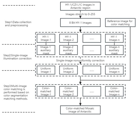
Figure 3.
Image color matching workflow.
3. Results
3.1. Image Nonuniformity Correction Results
Figure 4 shows an example of image brightness nonuniformity correction in the Antarctic coastal zone. Figure 4b is the correction result obtained using a common MASK method. There are luminance correction anomalies at the land-sea boundary in this result. Figure 4c shows the land-sea reference mask, which is obtained by setting a threshold T to distinguish the light and dark objects in Figure 4a. Figure 4d shows the results after using the land-sea auxiliary mask, and the results show that the method can improve the brightness correction anomaly in the land-sea boundary area and obtain a better correction effect.
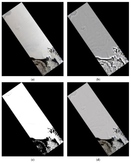
Figure 4.
Comparison of the brightness nonuniformity correction effect after the introduction of the land–sea reference mask: (a) original image, (b) common MASK method results, (c) land-sea auxiliary mask, and (d) results after the introduction of a reference mask.
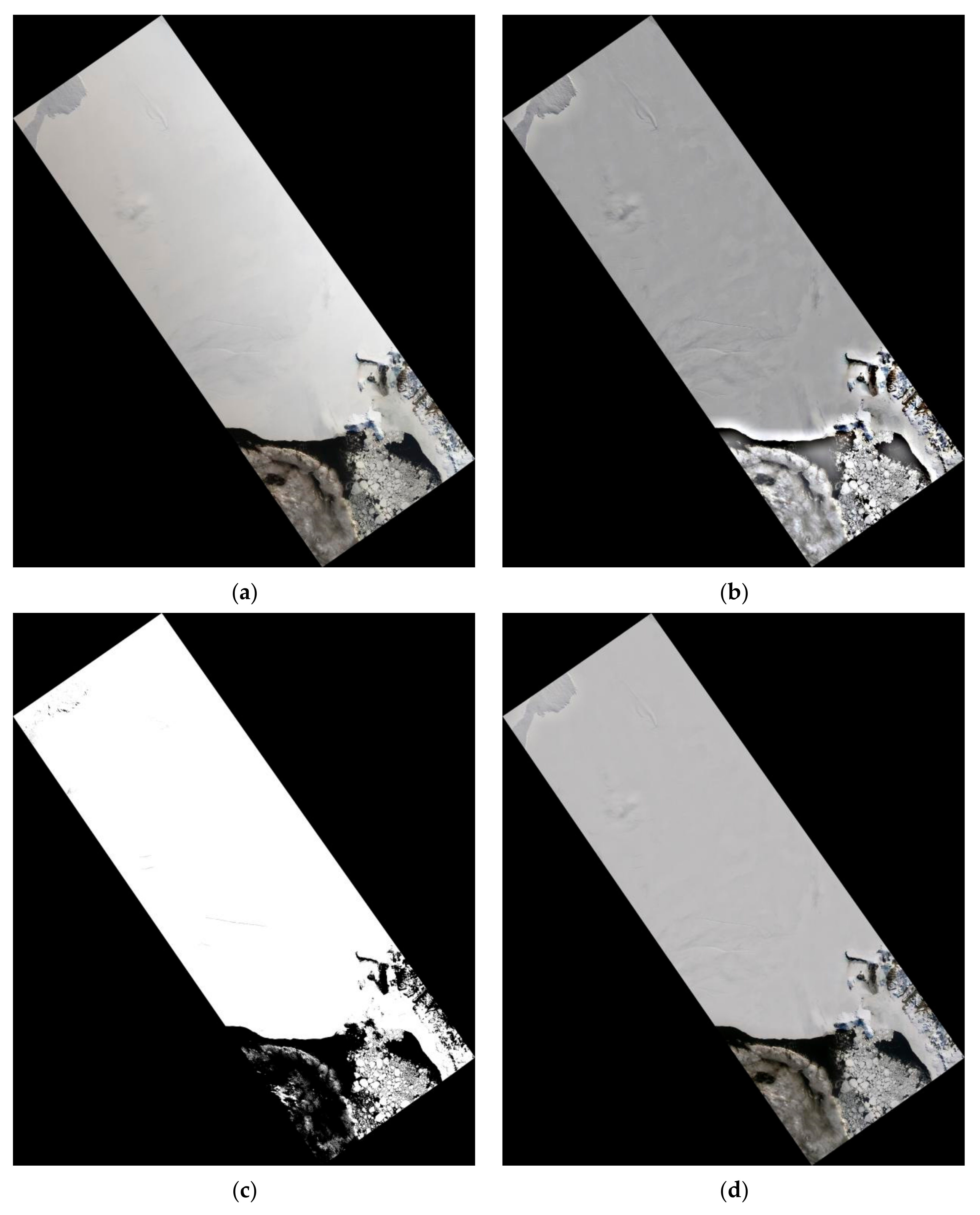
Figure 5 shows two other HY-1/CZI images with obvious nonuniformity phenomena in an inland Antarctic region. It can be seen from the corrected results that the nonuniform effect of brightness is obviously eliminated visually, and the brightness of the whole scene is basically evenly distributed. Table 3 shows the standard deviations of the above three images before and after correction. The statistical results show that the standard deviation after correction is basically less than that before correction, which further indicates that the uniformity of the corrected image is better than that of the original image.
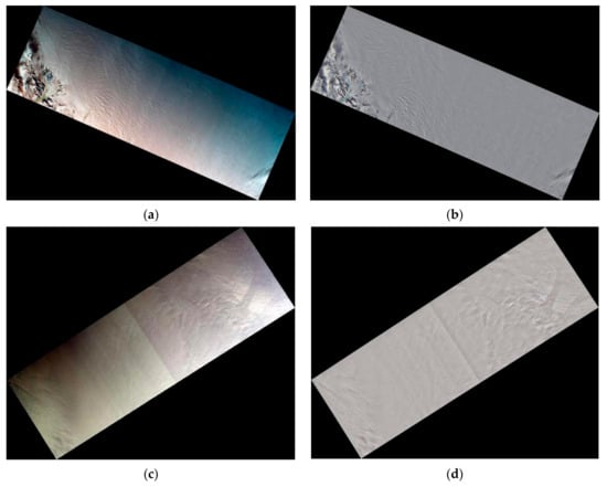
Figure 5.
Comparison of the HY-1/CZI brightness nonuniformity correction for Antarctic images: (a) original CZI image, (b) nonuniformity correction results of (a), (c) original CZI image, and (d) nonuniformity correction results of (c).
Table 3.
Statistical results before and after image nonuniformity correction.
3.2. Multi-Image Color Match Results
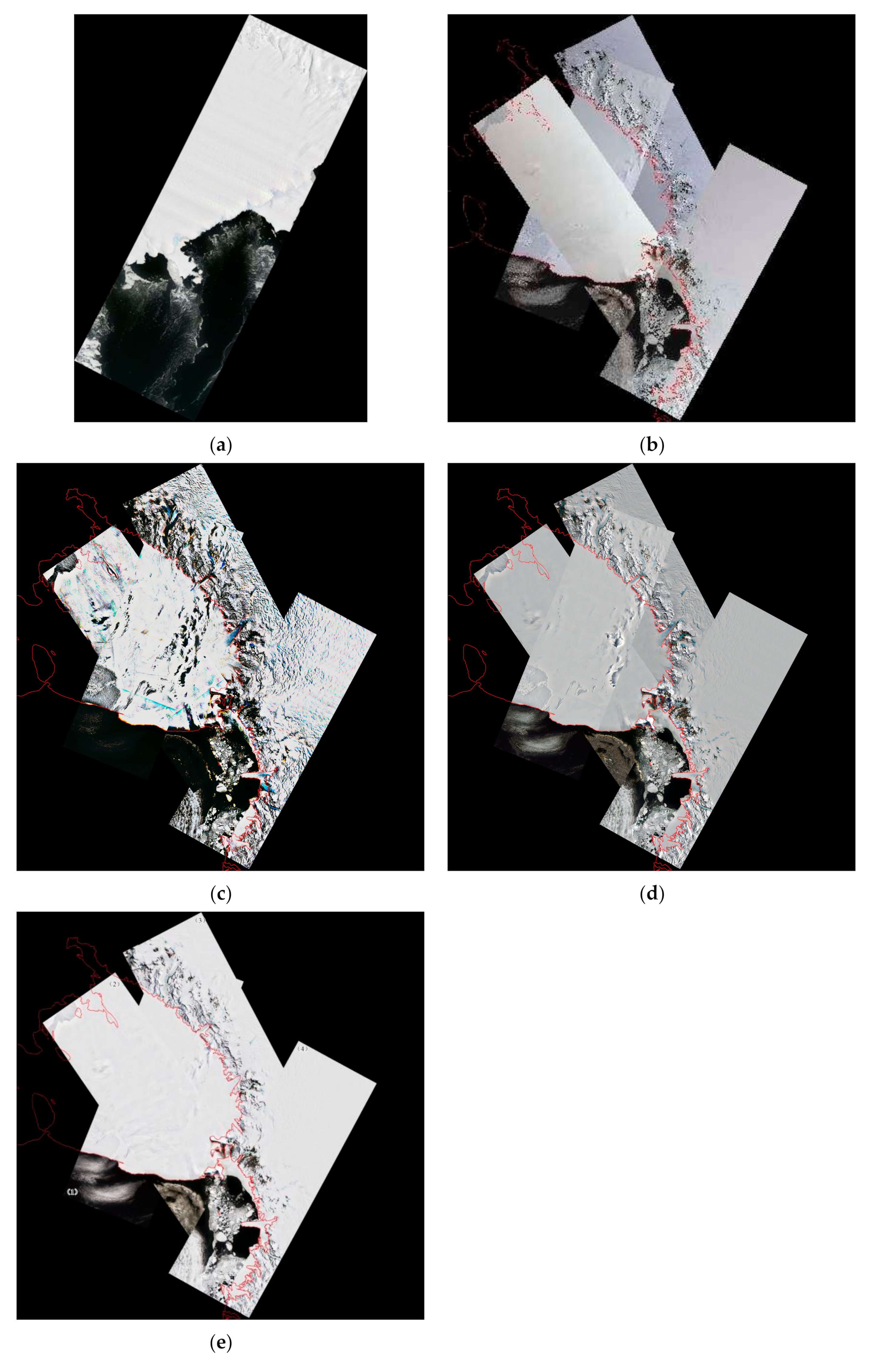
Four satellite images from HY-1/CZI cover the area around the Ross Ice Shelf in Antarctica. These images were taken on different dates in December 2021. Due to the differences in orbital characteristics and illumination conditions during the imaging process, obvious color differences existed in the original mosaic image from the visual effect (Figure 6b). The choice of reference image can be based on the principle of better visualization, and Figure 6a was chosen as the reference CZI Antarctic image for the next step of color matching. Figure 6e is the result from our algorithm, and the threshold value T = 90 was set in the process of color matching. After color matching for the four images, the color difference between the images was significantly improved, the brightness and color of the whole mosaic image were relatively uniform, and the visual effect was effectively improved. In this experiment, we also use the general histogram specification [42] and Wallis method [20] for comparison. The general histogram specification result is shown in Figure 6c. It can be seen that the contrast becomes larger in the glacial regions. Figure 6d shows the results using the Wallis algorithm. It can be seen that the color difference between the four images has been improved appropriately, but it remains significantly different from the color of the reference image.
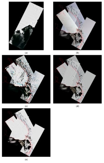
Figure 6.
Color matching results of the HY-1/CZI Antarctic image (the red line in the figure is the coastline): (a) reference image used for color matching, (b) original mosaic image, (c) general histogram specification result, (d) Wallis result, and (e) color-matching result of this paper.
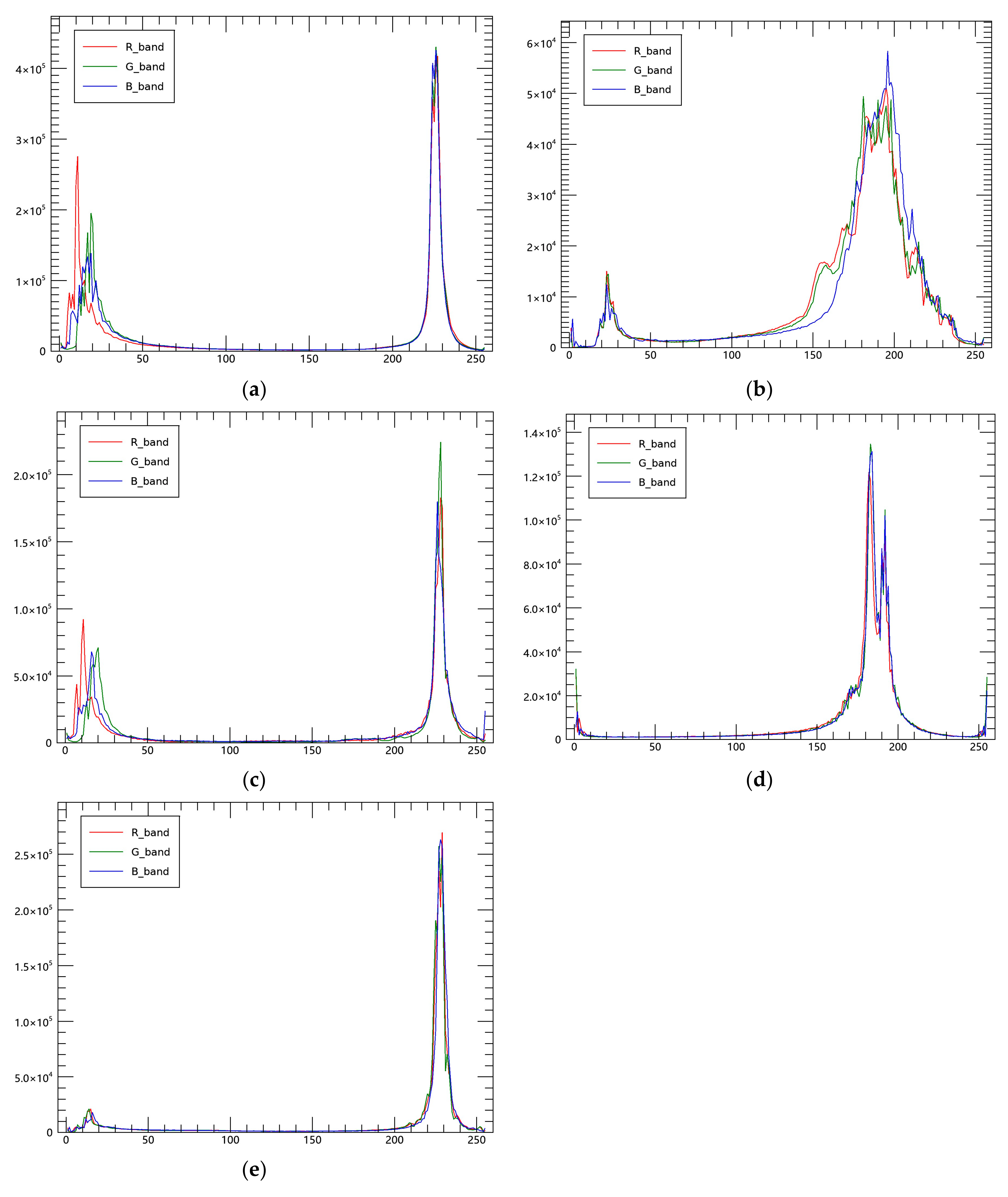
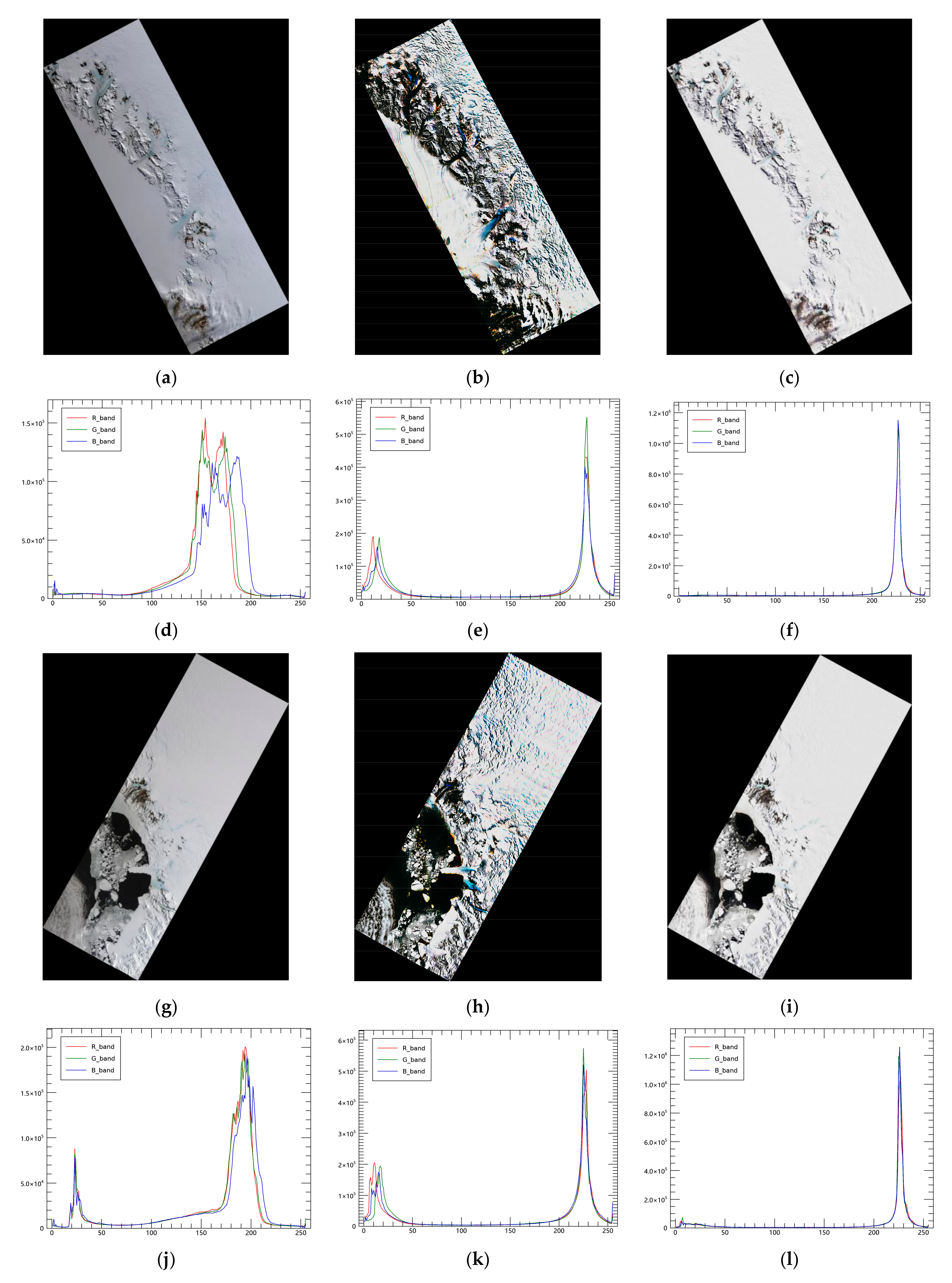
Figure 7 shows the histograms of the reference image, original mosaic image, and mosaic image after color matching. There is an obvious difference in the distribution of gray values between the water body and the glacier in the reference image from the histogram statistics results, which also indicates the obvious difference between the low reflectance of sea and the high reflectance of glaciers in the optical image of polar regions. Figure 7b shows the histogram of the original mosaic image without color matching. Due to the different color tones of each image, the distribution width of gray values from sea and glaciers is larger in the histogram than that of Figure 7a. Figure 7c–e are the histograms of the general histogram specification results, the Wallis matching results, and the results of this paper, respectively. Figure 7c,e show the histogram results after image color matching, which are in better agreement with the histogram distribution of the reference image (Figure 7a). The difference between Figure 7c,e is the difference in the number of pixel distributions between the two wave peaks on the histograms. There are more dark pixels in Figure 7c, because the general histogram specification method stretches some pixels on the glacier to dark pixels, thereby increasing the color contrast on the glacier (Figure 6c). In this paper, the darker and brighter targets are corrected by setting thresholds to make the color and contrast of the glaciers more natural. Figure 7d shows that the distribution value of the brighter region (glacier) in the Wallis result is lower than that in the reference image, so the glacier in the Wallis result is darker than that in the reference image.
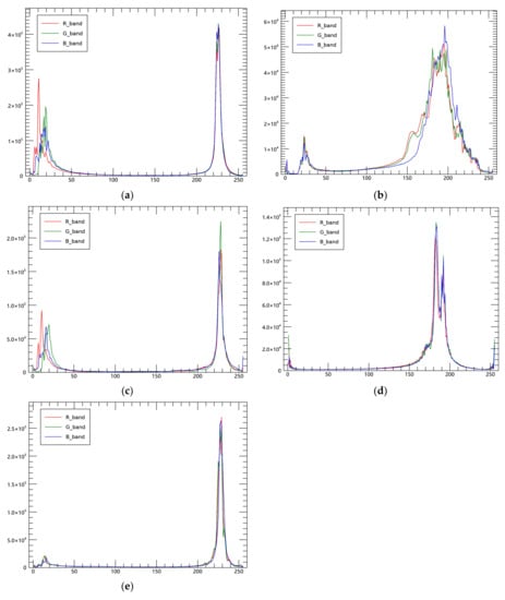
Figure 7.
Histogram comparison before and after color matching: (a) reference image histogram, (b) original mosaic image histogram, (c) histogram of the general histogram specification results, (d) Wallis results histogram, and (e) histogram of the paper results.
Table 4 analyzes the time efficiency of the different methods. The calculation time of the proposed method is comparable to that of the traditional histogram matching method, and the Wallis method has the highest processing efficiency, which may be due to the difference in computing efficiency caused by the Wallis method based on matrix calculation, while the other two methods are based on the mapping relationship of pixel values.
Table 4.
Running times for different color-matching algorithms.
4. Analysis and Discussion
4.1. Image Quality Analysis
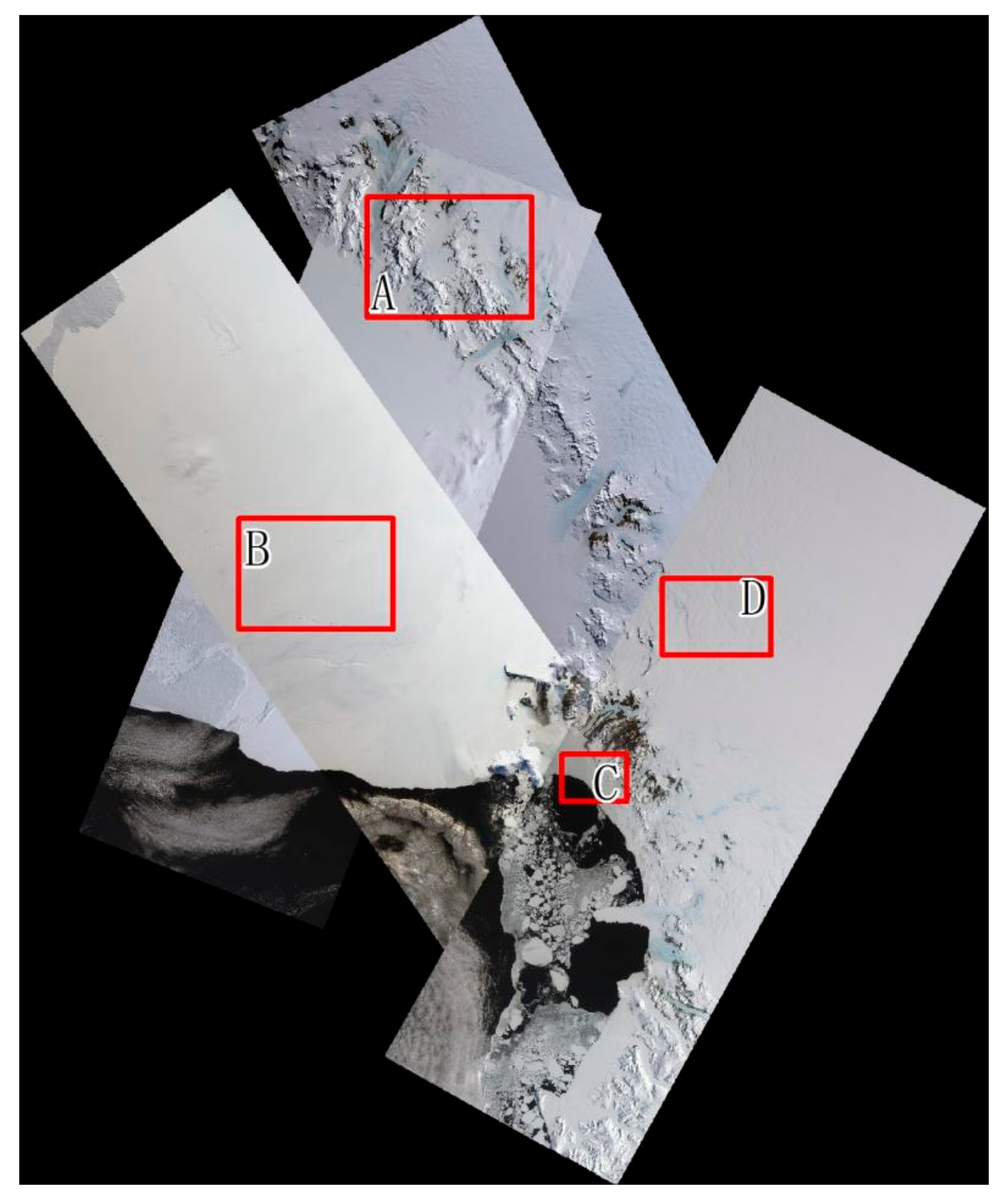
The mean value and standard deviation of an image can be used as objective indexes for image quality evaluation [43]. To conduct a quantitative analysis of the color-matching effect, four overlapping regions of images (A, B, C, D in Figure 8) are selected for evaluation according to the features of the image coverage area. The gray mean difference and the standard deviation difference of each image’s overlap areas were introduced to evaluate the quality [20], and the formula is as follows:
where and are the gray values of the two overlapping images, are the mean values of the images in two overlapping areas, and M and N are the number of rows and columns of the image, respectively. indicates the color difference between images. The smaller is, the smaller the color difference between images is, and the better the visual effect is. indicates the contrast difference between images; the smaller the value is, the smaller the contrast difference is.

Figure 8.
Overlapping regions (A, B, C, D) used for image quality evaluation.
Table 5 shows the statistical results of the above four areas. It can be seen from the results that the values obtained by the general histogram specification and Wallis methods are larger than the values of the original images in some regions, indicating that the two general methods do not significantly improve the color difference in these regions. However, the value by the method of this paper in the four areas is significantly smaller than that of the original image, which indicates that the color difference between the images after color matching is obviously less than the color difference between the original images, and the algorithm effectively eliminates the color difference between the images.
Table 5.
Statistical results of image color matching.
According to the statistical results of , the general histogram specification method reduces the contrast difference in region A, and the Wallis method decreases the contrast difference in region B. For the method adopted in this paper, the result for images B and D is smaller than that of the original image, which indicates that the contrast difference between regions B and D after color matching is small. The result for images A and C is greater than that of the original image, indicating that the contrast difference of the image after color matching is increased. The main reason for this is that the reference image used for color-matching processing increases the gray difference between low-reflectance objects (such as sea, bare rock, or shadows) and high-reflectance objects (such as glaciers). However, there are mountain shadows and bare rock areas in region A and a large amount of water area in region C, which have lower gray values than glaciers. As a result, the distribution contrast of the image gray value in regions A and C is increased after color matching.
The average gradient is another image quality index, which reflects the detailed information of the image and indicates the richness of the detail contrast [21,39]. The calculation formula is as follows:
where is the average gradient; and represent the pixel gradient in the row and column directions, respectively and M and N are the row and column numbers of the image, respectively. Generally, the larger the average gradient is, the larger the image contrast is and the more details the image contains, but the ideal image should retain rich texture information and reasonable contrast, not excessive contrast.
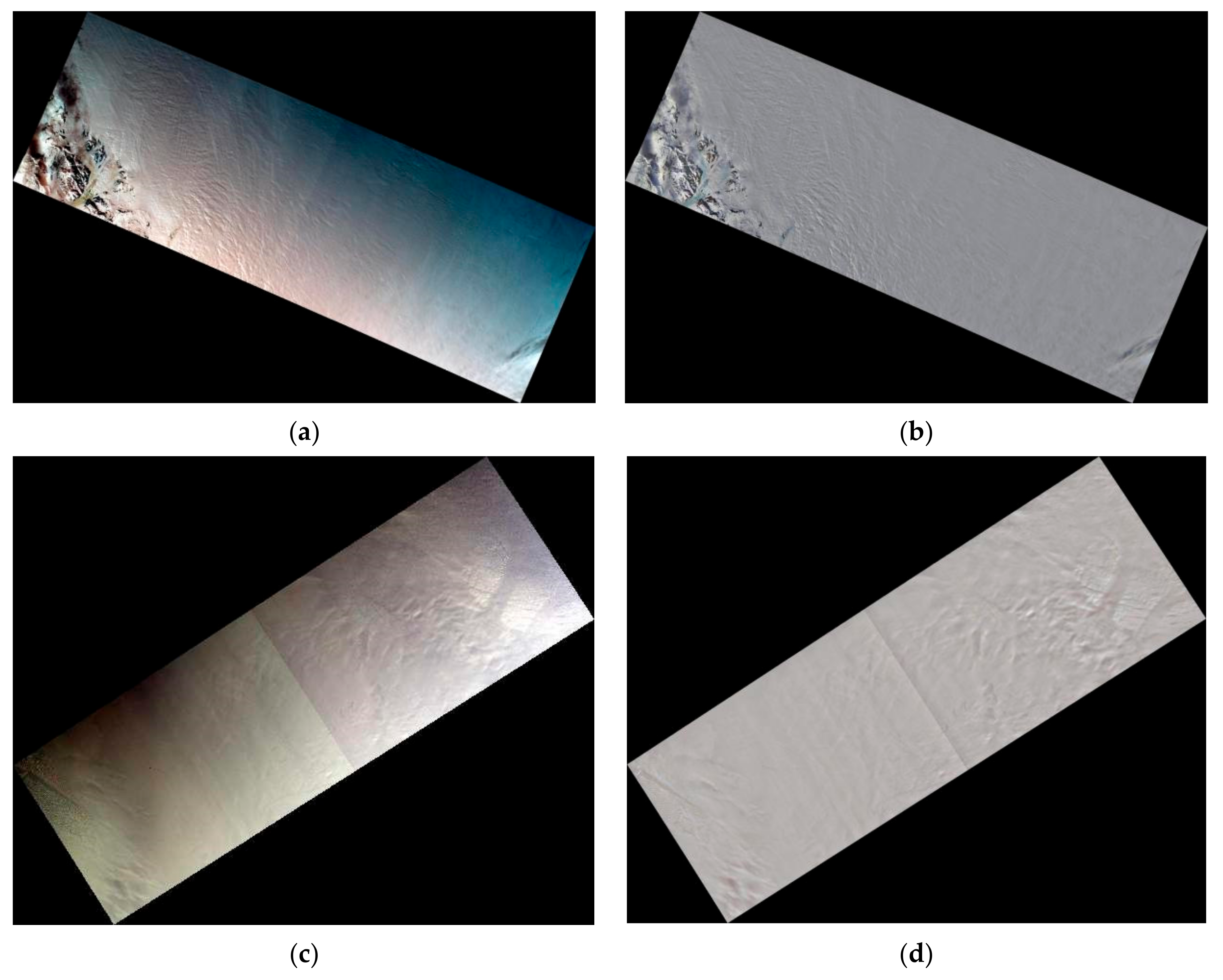
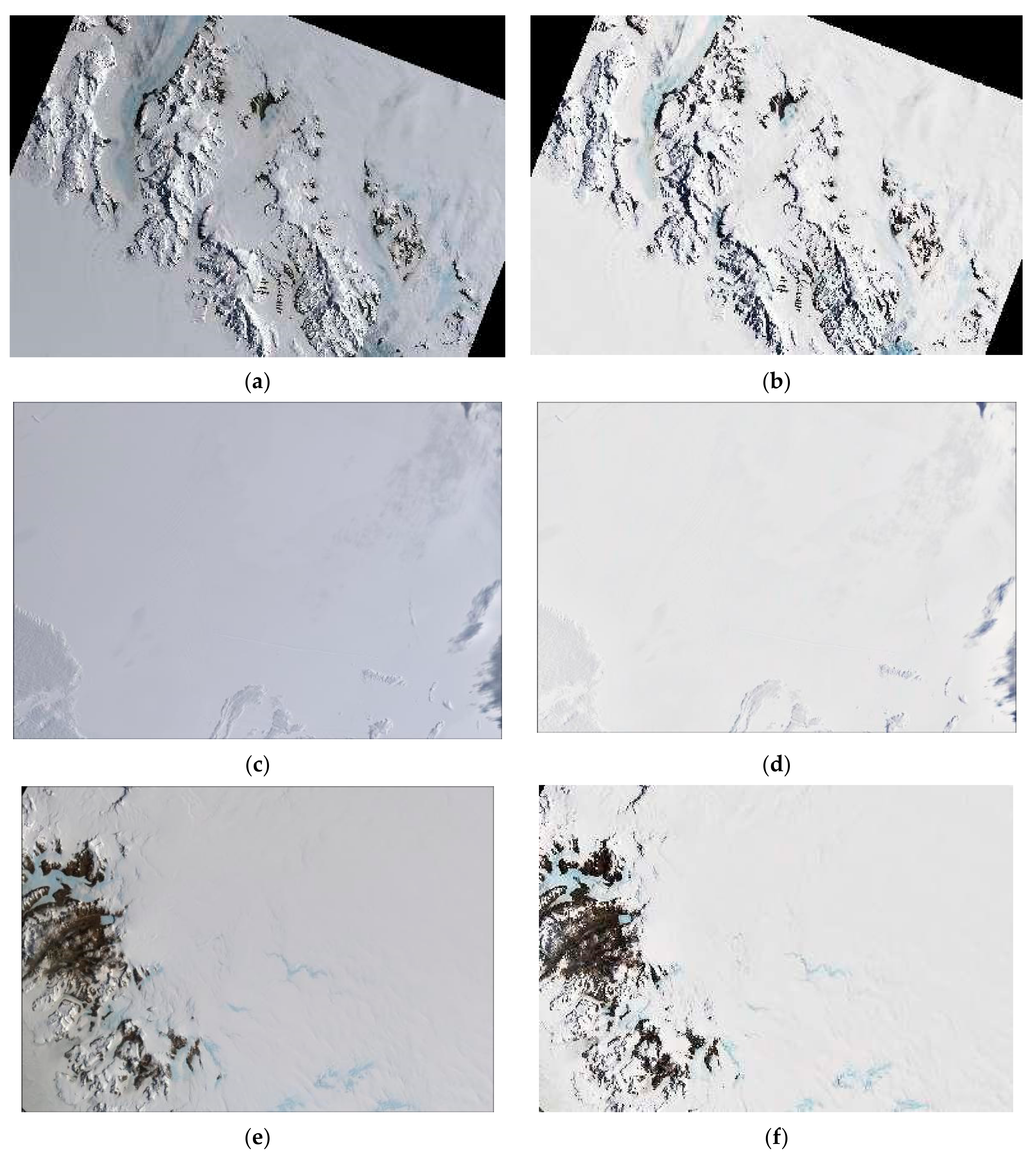
Figure 9 shows a comparison between the original image and the color-matched results of this study in some detailed areas. These sample areas include the typical feature distribution of Antarctica, including glaciers, mountains, bare rocks, and blue ice. After color matching, the colors of the resulting images have good consistency.
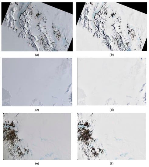
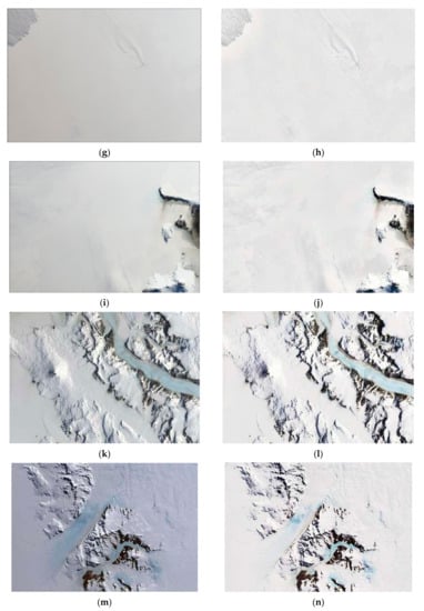
Figure 9.
Detailed comparison between the images before and after image color matching: (a) original detail image-1, (b) study result of image-1, (c) original detail image-2, (d) study result of image-2, (e) original detail image-3, (f) study result of image-3, (g) original detail image-4, (h) study result of image-4, (i) original detail image-5, (j) study result of image-5, (k) original detail image-6, (l) study result of image-6, (m) original detail image-7, and (n) study result of image-7.
Table 6 shows the average gradient values before and after color matching of the above seven feature sample areas. The statistical results show that the average gradient of each image after color matching is increased appropriately compared with the original image, which indicates that the details and contrast of the resulting image are enhanced to a certain extent.
Table 6.
Statistics of the average gradient before and after image color matching.
4.2. Overstretching in the Color-Matching Process
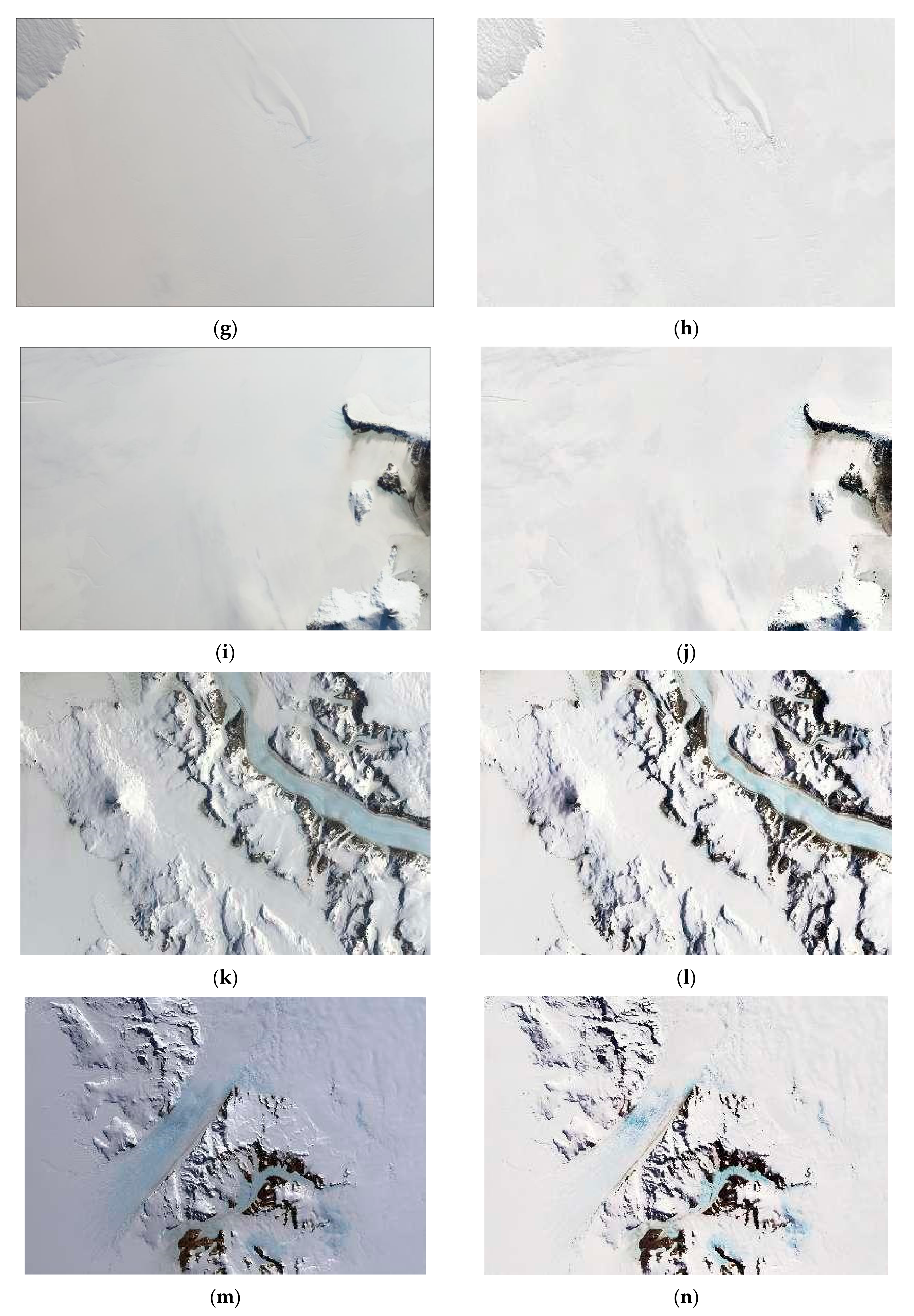
During color matching, this study is based on a histogram specification matching method, which generally has a good matching effect in images with rich ground object types and uniform gray distribution ranges. However, for the Antarctic region, the type of ground features is relatively simple, and the brightness difference is obvious in the optical images. As a result, a general histogram specification method will cause the color of the image to become unreal. In this research, to avoid unreal visual effects caused by such overstretching phenomena, we introduced a threshold value T to perform segmentation matching for different types of ground objects. Figure 10 shows the visual effect of the color-matching results for two landscape images with different T values. Below each image are the corresponding histogram distributions.
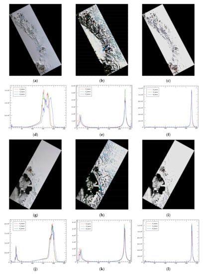
Figure 10.
Image matching comparison under different threshold values: (a) original image-1, (b) general method result of image-1 (T = 0), (c) study result of image-1 (T = 90), (d–f) are the corresponding histograms of (a–c), (g) original image-2, (h) general method result of image-2 (T = 0), (i) study result of image-2 (T = 90), and (j–l) are the corresponding histograms of (g–i).
It can be seen from the matching results in Figure 10 that the general histogram specification method and the proposed method both obtain relatively consistent histograms. However, the proposed method is more consistent with polar visual effects than general methods; the general method has greater contrast in the glacier area, and this visual effect is also confirmed by the statistical values of the average gradient (Table 7). It can be seen from the statistical results that the average gradient value of the general method is significantly higher than that of the original image, which indicates that the general method has caused excessive texture information and contrast in the matching results of this area. The method used in this paper is slightly higher than the original image, indicating that the contrast of the original image has been enhanced to a certain extent, and the visual effect is more reasonable.
Table 7.
Image color-matching average gradient value statistics.
5. Conclusions
In this paper, images from China’s Haiyang-1 satellite Coastal Zone Imager (CZI) were used to study the color uniformity of mosaic images in Antarctica based on MASK illumination simulation theory and image color matching via histogram specification matching. For a single image, a method based on MASK theory combined with an auxiliary mask was used, and the uneven illumination effect of the image was effectively eliminated. In the process of multiple-image color matching, a segmental color-matching method based on the threshold value is proposed for the Antarctic region. Compared with the results of the traditional histogram matching method and the Wallis method, the results obtained by the traditional histogram method and the method in this paper are closest to the histogram of the reference image, but the color distortion of the traditional histogram method is serious, and the results of the Wallis method show that the gray value distribution of the glacier target is lower than that of the reference image. The method in this paper is the best at eliminating the color difference between the images and the overall visual effect. Quantitative evaluation shows that the proposed method achieves good results in eliminating color differences in multiple images, while achieving a good balance between increasing image detail and improving visual effects.
Author Contributions
Conceptualization, T.Z.; data curation, T.Z. and Y.Z.; funding acquisition, L.S.; methodology, T.Z., L.H. and H.Z.; resources, L.S.; software, T.Z.; validation, L.H., H.Z. and X.Y.; visualization, Y.Z., H.Z. and X.Y.; writing—original draft, T.Z.; writing—review and editing, L.S. All authors have read and agreed to the published version of the manuscript.
Funding
This research was funded by the National Key Research and Development Program of China under Grant 2021YFC2803300 and the Antarctic Geographic Information Investigation.
Data Availability Statement
The data presented in this study are available on request from the author.
Conflicts of Interest
The authors declare no conflict of interest.
References
- Moghimi, A.; Celik, T.; Mohammadzadeh, A. Tensor-based keypoint detection and switching regression model for relative radiometric normalization of bitemporal multispectral images. Int. J. Remote Sens. 2022, 43, 3927–3956. [Google Scholar] [CrossRef]
- Li, J.; Hu, Q.; Ai, M. Optimal Illumination and Color Consistency for Optical Remote-Sensing Image Mosaicking. IEEE Geosci. Remote Sens. Lett. 2017, 14, 1943–1947. [Google Scholar] [CrossRef]
- Liu, J.; Ye, X.; Lan, Y. Remote sensing big data from Chinese ocean satellites and its application service. Big Data Res. 2022, 8, 75–88. [Google Scholar]
- Jezek, K.C.; Sohn, H.G.; Noltimier, K.F. “The RADARSAT Antarctic Mapping Project,” IGARSS’98. Sensing and Managing the Environment. In Proceedings of the 1998 IEEE International Geoscience and Remote Sensing. Symposium Proceedings. (Cat. No.98CH36174), Seattle, WA, USA, 6–10 July 1998; Volume 5, pp. 2462–2464. [Google Scholar] [CrossRef]
- Jezek, K.C.; Farness, K.; Carande, R.; Wu, X.; Labelle-Hamer, N. RADARSAT 1 Synthetic Aperture Radar Observations of Antarctica: Modified Antarctic Mapping Mission, 2000. Radio Sci.-RADIO Sci. 2003, 38, 32-1–32-7. [Google Scholar] [CrossRef]
- Jezek, K. RADARSAT-1 Antarctic Mapping Project: Change-detection and surface velocity campaign. Ann. Glaciol. 2002, 34, 263–268. [Google Scholar] [CrossRef]
- Bindschadler, R.; Vornberger, P.; Fleming, A.; Fox, A.; Mullins, J.; Binnie, D.; Paulsen, S.J.; Granneman, B.; Gorodetzky, D. The Landsat Image Mosaic of Antarctica. Remote Sens. Environ. 2008, 112, 4214–4226. [Google Scholar] [CrossRef]
- Feng, M.H.; Xiao, C.; Yan, L.; Jing, K.; Xin, Q.L. High-Resolution Remote Sensing Mapping of Antarctica; China Ocean Press: Beijing, China, 2021. [Google Scholar]
- Scambos, T.A.; Haran, T.M.; Fahnestock, M.A.; Painter, T.H.; Bohlander, J. MODIS-based Mosaic of Antarctica (MOA) data sets: Continent-wide surface morphology and snow grain size. Remote Sens. Environ. 2007, 111, 242–257. [Google Scholar] [CrossRef]
- Feng, M.H.; Xiao, C.; Yan, L.; Yan, M.Z.; Yu, F.Y.; Xian, W.W. An improved Landsat Image Mosaic of Antarctica. Sci. China (Earth Sci.) 2013, 56, 1–12. [Google Scholar] [CrossRef]
- Hui, F.; Ci, T.; Cheng, X.; Scambo, T.; Liu, Y.; Zhang, Y.; Wang, K. Mapping blue-ice areas in Antarctica using ETM and MODIS data. Ann. Glaciol. 2014, 55, 129–137. [Google Scholar] [CrossRef]
- Mathew, R.; Schwaller; Colin, J.; Southwell; Emmerson, L.M. Continental-scale mapping of Adélie penguin colonies from Landsat imagery. Remote Sens. Environ. 2013, 139, 353–364. [Google Scholar] [CrossRef]
- Campbell, G.G.; Pope, A.; Lazzara, M.; Scambos, T.A. The coldest place on Earth: 90 °C and below in East Antarctica from Landsat 8 and other thermal sensors. In Abstract C21D-0678 Presented at the 2013 Fall Meeting, AGU, San Francisco, CA, USA, 9–13 December 2013; AGU: San Francisco, CA, USA, 2013. [Google Scholar]
- Scambos, T.A.; Campbell, G.G.; Pope, A.; Haran, T.; Muto, A.; Lazzara, M.; Reijmer, C.H.; Broeke, M.R.v.D. Ultralow surface temperatures in East Antarctica from satellite thermal infrared mapping: The coldest places on Earth. Geophys. Res. Lett. 2018, 45, 6124–6133. [Google Scholar] [CrossRef]
- Shen, Q.; Wang, H.; Shum, C.K.; Jiang, L.; Hsu, H.T.; Dong, J. Recent high-resolution Antarctic ice velocity maps reveal increased mass loss in Wilkes Land, East Antarctica. Sci. Rep. 2018, 8, 4477. [Google Scholar] [CrossRef] [PubMed]
- Mukherjee, D.; Jonathan Wu, Q.M.; Wang, G. A comparative experimental study of image feature detectors and descriptors. Mach. Vis. Appl. 2015, 26, 443–466. [Google Scholar] [CrossRef]
- Forero, M.G.; Mambuscay, C.L.; Monroy, M.F.; Miranda, S.L.; Méndez, D.; Valencia, M.O.; Selvaraj, M.G. Comparative Analysis of Detectors and Feature Descriptors for Multispectral Image Matching in Rice Crops. Plants 2021, 10, 1791. [Google Scholar] [CrossRef]
- Sharma, S.K.; Jain, K.; Shukla, A.K. A Comparative Analysis of Feature Detectors and Descriptors for Image Stitching. Appl. Sci. 2023, 13, 6015. [Google Scholar] [CrossRef]
- Li, X.; Feng, R.; Guan, X.; Shen, H.; Zhang, L. Remote Sensing Image Mosaicking: Achievements and Challenges. IEEE Geosci. Remote Sens. Mag. 2019, 7, 8–22. [Google Scholar] [CrossRef]
- Li, S. Research on the Optimization of Color Consistency Processing and Seamline Determination of Remote Sensing Image. Ph.D. Thesis, Information Engineering University, Zhengzhou, China, 2018. [Google Scholar]
- Li, Z.; Zhu, H.; Zhou, C.; Cao, L.; Zhong, Y.; Zeng, T.; Liu, J. A Color Consistency Processing Method for HY-1C Images of Antarctica. Remote Sens. 2020, 12, 1143. [Google Scholar] [CrossRef]
- Wang, M.; Pan, J. A Method of Removing the Uneven Illumination for Digital Aerial Image. J. Image Graph. 2004, 9, 104–108+127. [Google Scholar]
- Sun, W.; You, H.; Fu, X.; Song, M. A non-linear MASK dodging algorithm for remote sensing images. Sci. Surv. Mapp. 2014, 39, 130–134. [Google Scholar] [CrossRef]
- Fan, C.N.; Zhang, F.Y. Homomorphic Filtering Based Illumination Normalization Method for Face Recognition. Pattern Recognit. Lett. 2011, 32, 1468–1479. [Google Scholar] [CrossRef]
- Rahman, Z.; Jobson, D.J.; Woodell, G.A. Multi-scale Retinex for Color Image Enhancement. IEEE Int. Conf. Image Process. 1996, 3, 1003–1006. [Google Scholar]
- Orsini, G.; Ramponi, Q.; Carrai, P.; Di, F.R. A Modified Retinex for Image Contrast Enhancement and Dynamics Control. Int. Conf. Image Process. 2003, 3, 393–396. [Google Scholar]
- Yu, X.; Fang, J.; Li, C.; Liao, M.; Chen, X. Comparative Study on Dodging Algorithms for A Single UAV Image. Geomat. World 2019, 26, 96–103. [Google Scholar]
- Helmer, E.H.; Ruefenacht, B. Erratum: Cloud-free satellite image mosaics with regression trees and histogram matching. Photogramm. Eng. Remote Sens. 2005, 71, 1079–1089. [Google Scholar] [CrossRef]
- Zhang, Q.; Zhang, Y.; Meng, Y. Research on Color Uniforming for Multi-source Remote Sensing Images Based on Histogram Matching Method. Geospat. Inf. 2020, 18, 54–57+7. [Google Scholar]
- Xie, R.; Xia, M.; Yao, J.; Li, L. Guided color consistency optimization for image mosaicking. ISPRS J. Photogramm. Remote Sens. 2018, 135, 43–59. [Google Scholar] [CrossRef]
- Schroeder, T.A.; Cohen, W.B.; Song, C.; Canty, M.J.; Yang, Z. Radiometric Correction of Multi-Temporal Landsat Data for Characterization of Early Successional Forest Patterns in Western Oregon. Remote Sens. Environ. 2006, 103, 16–26. [Google Scholar] [CrossRef]
- Nielsen, A.A. The Regularized Iteratively Reweighted MAD Method for Change Detection in Multi- and Hyperspectral Data. IEEE Trans. Image Process. 2007, 16, 463–478. [Google Scholar] [CrossRef] [PubMed]
- Velloso, M.L.F.; Souza, F.J.D. Non-Parametric Smoothing for Relative Radiometric Correction on Remotely Sensed Data. In Proceedings of the IEEE XV Brazilian Symposium on Computer Graphics and Image Processing, Fortaleza, Brazil, 10 October 2002; pp. 83–89. [Google Scholar]
- Palubinskas, G.; Muller, R.; Reinartz, P. Mosaicking of Optical Remote Sensing Imagery. In Proceedings of the IEEE International Geoscience and Remote Sensing Symposium, Toulouse, France, 21–25 July 2003; pp. 3955–3957. [Google Scholar]
- Pan, J.; Wang, M.; Li, D.R. A Network-Based Radiometric Equalization Approach for Digital Aerial Ortho Image. IEEE Geosci. Remote Sens. Lett. 2011, 7, 401–405. [Google Scholar] [CrossRef]
- Li, L.; Xia, M.; Liu, C.; Li, L.; Wang, H.; Yao, J. Jointly optimizing global and local color consistency for multiple image mosaicking. ISPRS J. Photogramm. Remote Sens. 2020, 170, 45–56. [Google Scholar] [CrossRef]
- Chen, L.; Ma, Y.; Lian, Y.; Zhang, H.; Yu, Y.; Lin, Y. Radiometric Normalization Using a Pseudo−Invariant Polygon Features−Based Algorithm with Contemporaneous Sentinel−2A and Landsat−8 OLI Imagery. Appl. Sci. 2023, 13, 2525. [Google Scholar] [CrossRef]
- Pan, J. The Research on Seamless Mosaic Approach of Stereo Orthophoto. Master’s Thesis, Wuhan University, Wuhan, China, 2005. [Google Scholar]
- Han, Y. Research on Key Technology of Color Consistency Processing for Digtial Ortho Map Mosaicing. Ph.D. Thesis, Wuhan University, Wuhan, China, 2014. [Google Scholar]
- Richards, J.A. Remote Sensing Digital Image Analysis; Springer: Berlin/Heidelberg, Germany, 1999; Volume 3. [Google Scholar]
- Yao, F.; Wan, Y.; Hu, H. Research on the Improved Image Dodging Algorithm Based on Mask Technique. Remote Sens. Inf. 2013, 28, 8–13. [Google Scholar] [CrossRef]
- Ruan, Q. Digital Image Processing; Publising House of Electronics Industy: Beijing, China, 2007. [Google Scholar]
- Liu, H. Research and Implementation of Remote Sensing Image Dodging Algorithm Based on IDL. Master’s Thesis, Hebei University of Engineering, Handan, China, 2018. [Google Scholar]

Disclaimer/Publisher’s Note: The statements, opinions and data contained in all publications are solely those of the individual author(s) and contributor(s) and not of MDPI and/or the editor(s). MDPI and/or the editor(s) disclaim responsibility for any injury to people or property resulting from any ideas, methods, instructions or products referred to in the content. |
© 2023 by the authors. Licensee MDPI, Basel, Switzerland. This article is an open access article distributed under the terms and conditions of the Creative Commons Attribution (CC BY) license (https://creativecommons.org/licenses/by/4.0/).