Abstract
Soil salinization is a severe soil degradation issue in arid and semiarid regions. The distribution of soil salinization can prove useful in mitigating soil degradation. Remote sensing monitoring technology is available for obtaining the distribution of soil salinization rapidly and nondestructively. In this study, experimental data were collected from seven study areas of the Hetao Irrigation District from July to August in 2021 and 2022. The soil salt content (SSC) was considered at various soil depths, and the crop type and time series were considered as environmental factors. We analyzed the effects of various environmental factors on the sensitivity response of unmanned aerial vehicle (UAV)-derived spectral index variables to the SSC and assessed the accuracy of SSC estimations. The five indices with the highest correlation with the SSC under various environmental factors were the input parameters used in modeling based on three machine learning algorithms. The best model was subsequently used to derive prediction distribution maps of the SSC. The results revealed that the crop type and time series did not affect the relationship strength between the SSC and spectral indices, and that the classification of the crop type and time series can considerably enhance the accuracy of SSC estimation. The mask treatment of the soil pixels can improve the correlation between some spectral indices and the SSC. The accuracies of the ANN and RFR models were higher than SVR accuracy (optimal R2 = 0.52–0.79), and the generalization ability of ANN was superior to that of RFR. In this study, considering environmental factors, a UAV remote sensing estimation and mapping method was proposed. The results of this study provide a reference for the high-precision prediction of soil salinization during the vegetation cover period.
1. Introduction
Soil salinization is a global issue that severely degrades soil resources and harms the environment. The sustainability of the ecological environment and food security is considerably degraded. Salinized soil has spread to cover an area of over 1 billion hectares worldwide [1]. Therefore, the precise and efficient acquisition of soil salinization information is critical for the prevention of soil salinization. As one of three large-scale irrigation areas in China, the Hetao Irrigation District (HID) has a high groundwater level and experiences severe secondary salinization because of the excessive diversion of water from the Yellow River and water leakage in the canal system [2].
Unmanned aerial vehicle (UAV) remote sensing technology has been proven to be suitable for inverting soil salinity in farmlands [3]. Compared with satellite remote sensing, UAVs can obtain high-resolution (centimeter-level) remote sensing images with less investment. Detection time is flexible and not limited by transit time. Therefore, UAVs have widely become used in the quantitative inversion of the SSC at the field scale [4]. The common types of monitoring sensors installed on UAVs include hyperspectral sensors [5], multispectral sensors [6], and LiDAR sensors [7]. Among them, the multispectral sensor is an ideal sensor for predicting the SSC because of its low price, simple data processing, and SSC-sensitive band. Among the various categories of spectral indices derived from multispectral sensors, the salinity index (SI) and vegetation index (VI) have been proven to achieve excellent performances in SSC inversion during the vegetation cover period [8]. However, the two categories of indices have many spectral indices, and the actual situation in the field is complex and heterogeneous. Therefore, the spectral indices sensitive to the SSC under various environmental conditions are yet to be determined. Therefore, conducting a correlation analysis of the spectral index according to various conditions is critical when estimating the SSC under various time series and crop types in the HID.
With irrigation and other field management practices, salt migrates horizontally or vertically in the soil and the amount of salt increases or decreases cumulatively. Therefore, when assessing the soil salinization level in a certain area, the monitoring of multiple time series of bare-land periods and vegetation cover periods can provide greater detail about the soil salinization level than a single time series. The monitoring results could be applied in a timely manner to field management and soil improvement. When SSC inversion is performed during the vegetation cover period, the response of the crop canopy spectral characteristics to the SSC is a critical monitoring indicator [8]. However, the factors affecting the phenotypic characteristics of the crop canopy not only include the SSC but also the crop type, crop variety, and physiological characteristics. Therefore, environmental factors should be considered in SSC inversion during the vegetation cover period, and some scholars have discussed the effect of environmental factors on the accuracy of SSC inversion [9]. Scudiero et al. [10] revealed that the field management type (collapsed and falling soils) and meteorological factors (the rain and temperature), as explanatory variables or additional explanatory variables, could enhance the accuracy of the SSC inversion models. Ivushkin et al. [11] revealed that the crop type affected the intensity of the relationship between the canopy temperature and the SSC by evaluating the correlation between the canopy temperature index (the vegetation index and brightness temperature) and the SSC. Li et al. [12] proved that the spectral indices of various time series have distinct sensitivity responses to the SSC and that selecting various spectral indices according to different time series (seasons) is necessary in order to model the SSC. These studies are based on satellite remote sensing and have meter-level image resolution. The effect of various crop types and time series on the spectral features derived from UAV images (at the centimeter level) should be demonstrated separately. Furthermore, the composite effect between environmental factors should be discussed.
Because of its excellent nonlinear problem fitting ability and high-dimensional data processing, the machine learning regression algorithm has been proven to outperform the linear model in SSC estimation because the relationship between the SSC and explanatory variables can be nonlinear due to the complex field environment [13]. The multilayer structure of the RF and ANN algorithms can express highly complex nonlinear relationships, and these methods are used in many SSC prediction and inversion studies [14,15]. SVR maps data to the infinite dimensional space through the use of the kernel function, thereby realizing the classification of nonlinear problems. The method is robust and has good generalization abilities, meaning that it is also a good choice for use in SSC modeling [16,17]. The same machine learning algorithm may not achieve a stable simulation accuracy when solving for the SSC under various conditions. Therefore, evaluating the ability of multiple machine learning regression algorithms is critical for modeling SSC prediction under various environmental factors.
The objectives of this study are to discuss whether the crop type and time series can affect the SSC estimation accuracy at diverse soil depths based on UAV remote sensing; to evaluate whether the mask processing of soil pixels can improve the correlation between SSC and spectral covariates; to analyze the sensitivity response of the spectral index to the SSC at diverse soil depths in order to determine the best estimated depth; and to evaluate the performance of three machine learning algorithms in order to solve SSC regression problems under diverse conditions, establish an optimal estimation model, and generate high-precision and high-resolution SSC prediction distribution maps.
2. Materials and Methods
2.1. Study Site
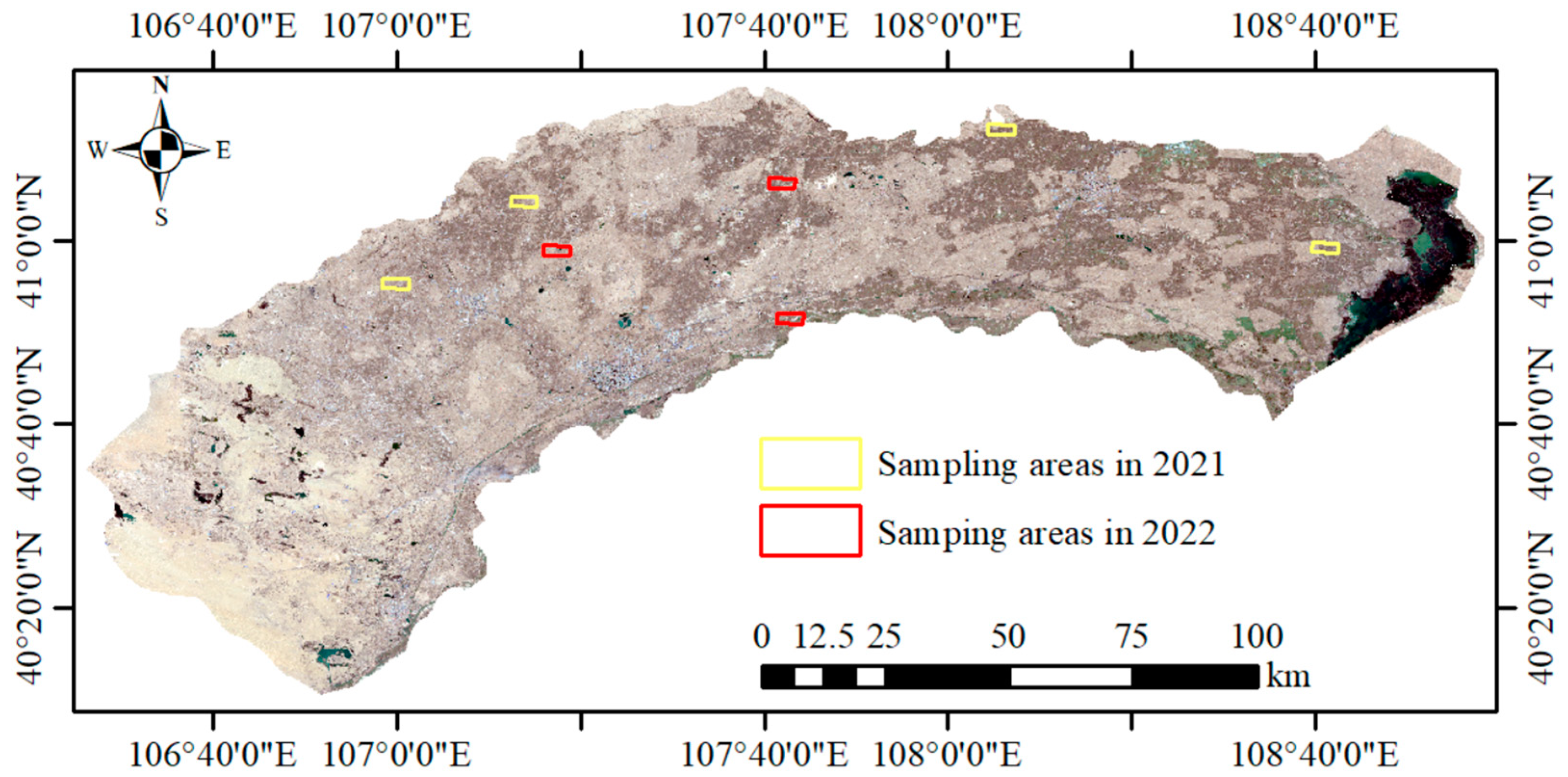
The experimental data of the study were collected from July to August in 2021 and 2022 in the HID (40°19′–41°18′N, 106°20′–109°19′E). The HID is located in the west of Inner Mongolia and the middle and upper reaches of the Yellow River basin, which are crucial grain production bases in China. The HID has abundant sunlight but low rainfall, and an annual evaporation rate 15–17 times that of precipitation. The terrain of the HID is flat, which has a tilt from southwest to north with a slope of 0.0125–0.02%. Perennial irrigation from the Yellow River has led to a more abundant distribution of irrigation-silted soil in the HID. In addition, the more commonly distributed soil types include meadow soil, desert soil, and chestnut soil. Therefore, agricultural production in the area strongly relies on water from the Yellow River. The irrigation area of the HID was 57.6 × 10⁴ ha in 2019, with the irrigated area of Yellow River diversion accounting for more than 90% of the total irrigated area [18]. Flood and drip irrigation methods are widely used in the HID. Perennial over-irrigation leads to high groundwater levels, and approximately two-thirds of the farmland has diverse degrees of salinization. In total, 45.5%, 16%, and 3.1% of farmland area exhibit mild, moderate, and severe salinization, respectively [19]. The HID has two irrigations every year, with a spring irrigation period in May and an autumn irrigation period during October and November. During the two periods, large-scale irrigation was observed within the entire irrigation area. According to the field survey results and the literature, maize, sunflower, wheat, and squash are the primary local crops [20]. In this study, seven study areas in the HID (Figure 1) were considered. Four areas were studied in 2021 and three areas were investigated in 2022. In each area, experimental data were collected twice a year, with collections in July and August.
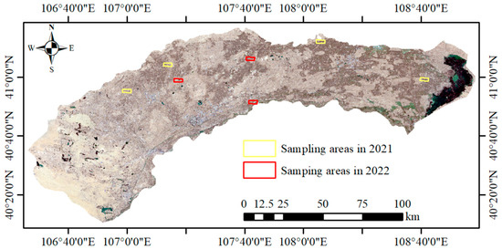
Figure 1.
Aerial maps of the study area.
2.2. Data Acquisition and Pretreatment
2.2.1. UAV Imagery
Multiple UAV spectral images were collected from seven study areas during clear and windless weather conditions in 2021 and 2022. The image acquisition platform was a self-developed UAV system equipped with a RedEdge five-band multispectral camera (MicaSense, Inc., Seattle, WA, USA). The UAV platform and detailed information on RedEdge are presented in [21]. The UAV was flown at noon between 11:00 and 13:30. Before each UAV flight, the calibrated reflectance panel was used to correct the camera spectrum, and the flight parameters were uniformly set, with specific settings according to [22]. Three ground control points were placed within each study area to improve the geographic location accuracy of UAV imagery. The collected single image was spliced using the Pix4DMapper (Pix4D Inc., Prilly, Switzerland), and manual identification method was used to clip the image of the areas not under consideration. An orthophoto of study areas was obtained with a resolution of 7.5 cm to the ground.
2.2.2. Spectral Indices Calculation
The spectral indices used in this study include VIs and SIs. All spectral indices were obtained via mathematical operations on two or more bands of the acquired multispectral image. Studies have proven the strong correlation between the VIs and SSC when monitoring soil salinization during the vegetation cover periods. Therefore, based on previous studies [23,24], 10 SIs and 10 VIs were used for the study. Table 1 presents the formulas for calculating these 20 spectral indices.

Table 1.
Spectral indices used in this study.
2.2.3. Ground-Truth Data Acquisition
The SSC ground truth was collected at the same time as the UAV imagery in the sampling area. The RTK positioning instrument (KOLIDA Instrument Co., Ltd., Guangzhou, Guangdong, China) was used to record the spatial geographic position coordinates of each sampling point. In accordance with the principles of uniform distribution, representativeness, and practical data gradient, 12–26 soil sampling points were set in each sampling area. Figure 2 shows the distribution of sampling points. The collection depth of soil samples was at two levels of 0–20 and 20–40 cm, and Table 2 presents the sampling time and quantity of the seven study areas. The collected soil samples were stored in various aluminum boxes and completely air-dried (~12 days). The samples were then ground into a powder with a granule diameter of 1 mm. Next, 20g of soil powder was added to 100 mL of distilled water to create a soil solution, and the solution was fully stirred using a magnetic mixer for complete mixing and subsequently left to settle for approximately 10 h. Finally, a conductivity meter (DDS-307A, Shanghai Yidian Scientific Instruments Co., Ltd. Shanghai, China) was used to measure the conductivity electrical conductivity (EC1:5) of the filtrate. The EC1:5 was converted to the SSC using an empirical Formula (1). The SSC of all sampling points was calculated to be 0.062–0.699%. Based on these values, soil was classified into no salinization, mild salinization, moderate salinization, and severe salinization based on the SSC ranges of 0.062–0.2%, 0.2–0.4%, 0.4–0.6%, and 0.6–0.699%, respectively [24].
SSC = (0.2882 × EC1:5 + 0.0183)
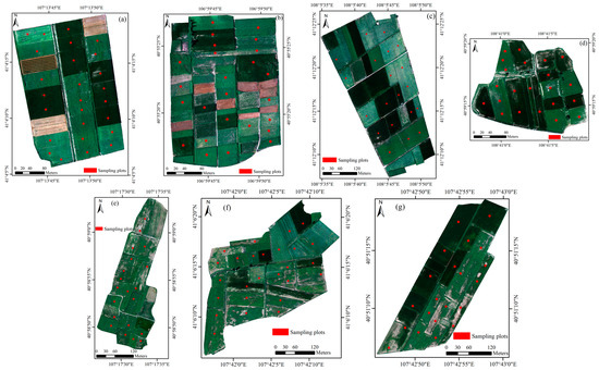
Figure 2.
Distribution maps of sampling plots for each study area: (a–d) are the study area 1–4 in 2021, (e–g) are the study area 5–7 in 2022.
Table 2.
Sampling time, quantity and soil salinization level statistics for each study area in 2021 and 2022.
2.3. Methods
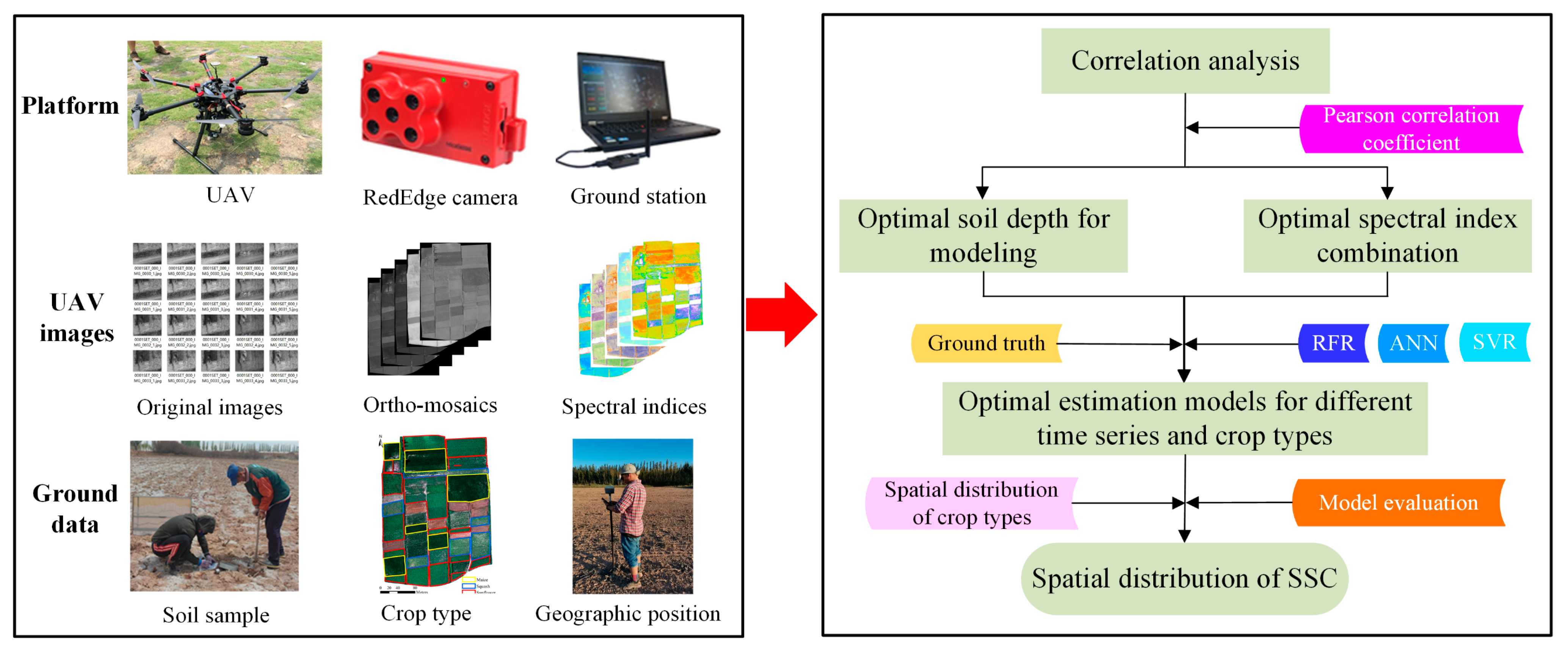
The research flow chart of this study is shown in Figure 3.

Figure 3.
Flow chart.
2.3.1. Variable Selection Method
The closeness degree of the correlation between explanatory variables and dependent variables is typically highly correlated with the accuracy of the regression model. The Pearson’s correlation coefficient (PCCs) can describe the linear correlation between two variables, and the r-value is used to express the correlation coefficient (calculation formula was given in [40]). A larger absolute value of r-value represents a stronger correlation. In this study, the heatmap was used to demonstrate the strength of the correlation between the spectral variables of diverse datasets and the SSC clearly.
2.3.2. Soil Pixels Mask Method
When monitoring soil salinity information under the cover of vegetation, the collected UAV images typically contain exposed soil pixels because of diverse fractional vegetation cover (FVC). Among soil pixels, with the exception of the soil constituent, diverse crop growth stages and crop types can also lead to differences in the exposed area of soil, which may affect the spectrum and spectral index errors within the sampling point range and affect monitoring accuracy. Studies have proved that a fixed NDVI threshold can be used to distinguish between the crop and soil pixels [14]. This study calculated the NDVI values of crop and soil pixels in the fields, planted sunflower, maize, and squash, and determined that the NDVI threshold was 0.4. The pixels with a lower NDVI value than 0.4 were determined to be soil pixels, and these pixels were masked using the binary mask method, as presented in [41]. Mask processing was performed in the R language (R-3.5.3).
2.3.3. Modeling and Evaluation Methods
According to previous studies, machine learning algorithms achieved excellent model accuracy in their application to SSC inversion [42,43]. Three machine learning regression methods, including RFR, ANN, and SVR, were used to establish SSC estimation models for diverse datasets. RFR is a deformation algorithm based on the decision tree method, and the number of decision trees and node variables were noted. After parameter optimization, the two parameters were optimized using values of 400 and 3, respectively. The ANN algorithm requires the selection of an appropriate network structure first. We selected a single hidden-layer feedforward backpropagation structure. The initial number per node and the weight per layer were optimized using values of 10 and 0.5. SVR is similar to ANN, requires the selection of the kernel function first, and then determines the penalty factor. The radial basis kernel function was selected as the kernel function, and the penalty parameter was optimized using values of 1.
Due to the limited quantity of data samples, and to avoid overfitting and other errors caused by the data distribution between different datasets as much as possible, the k-fold cross-validation method [44] was used for model training and testing. The parameter k of cross-validation was set to 3, which revealed that the data were divided into three parts. Two parts of the data (two-thirds) comprised calibration dataset for training each time, and the remaining portion of data (one-third) was used as the validation dataset for testing. The aforementioned treatment was repeated three times, and average values were considered to be the final results. Root-mean-square error (RMSE), determination coefficient (R2), Lin’s concordance correlation coefficient (LCCC) and ratio of performance to deviation (RPD) were taken as indicators with which to evaluate models, and the calculation formulas of the R2 and RMSE, detailed in [45], were referred to. Smaller RMSE and larger R2 values result in better model performance. LCCC is a standard used to evaluate the consistency of predicted and observed values [46], and RPD can evaluate the predictability of a model [47]. An RPD ≤ 1.5 predicts poorly, 1.5 ≤ RPD < 2 predicts well, and an RPD > 2 predicts very well. An LCCC > 0.9 denotes excellent agreement, one from 0.80 to 0.90 suggests substantial agreement, a value between 0.65 and 0.80 indicates moderate agreement, and an LCCC ≤ 0.65 suggests poor agreement. The R language was used for modeling, cross-validation, and model evaluation. RFR, ANN, and SVR were completed using the “randomForest,” “nnet,” and “e1071” packages, respectively, and cross-validation was completed using the “caret” package.
3. Results
3.1. Soil Mask Analysis
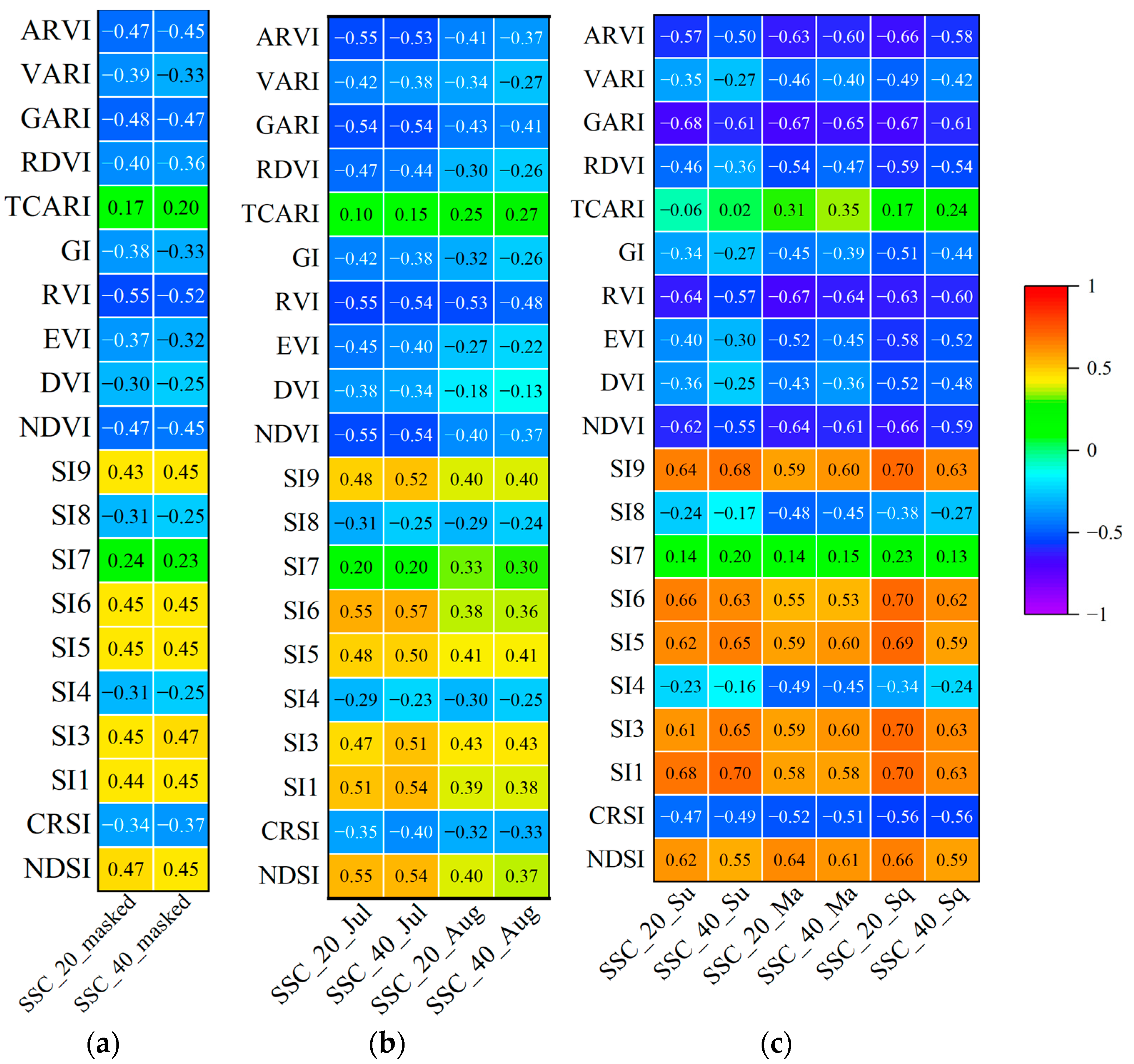
In this study, in order to determine whether bare soil pixels in UAV images affect the response degree of spectral index variables to the SSC, the threshold method was used to mask the original UAV imagery of each band and remove soil pixels. The PCCs analysis was performed between spectral indices (images removed the soil pixels and original images) and the SSC ground-truth value. The analysis results are presented in Figure 4. For SSC with different soil depths, mask treatment improved the correlation of some spectral indices. For example, the r-values of TCARI were increased by 0.16 and 0.17 with 0–20 and 20–40 cm SSC datasets. However, the correlation between another part of the spectral index and the SSC was not considerably improved using mask treatment, and even decreased to some extent. For example, the r-value between CRSI and the SSC was reduced by 0.05 using mask treatment at 0–20 cm. And we also noticed that, when the relation between spectral indices and the SSC was moderately correlated (r-value greater than 0.4), mask treatment could promote the response degree of these spectral indices (NDSI, SI1, SI5, SI6, NDVI, etc.) to SSC. We observed that the promotion effect of mask treatment on 0–20 cm and 20–40 cm SSC was almost synchronous. When the correlation between spectral indices and 0–20 cm SSC was increased using mask treatment, the correlation degree between 20–40cm SSC and spectral indices generally increased synchronously and vice versa.
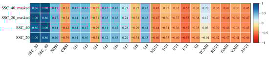
Figure 4.
Correlation coefficient (r) between SSC and spectral indices of the original and masked imagery.
3.2. Statistical Analysis of SSC and Spectral Index of Various Crop Types and Time Series
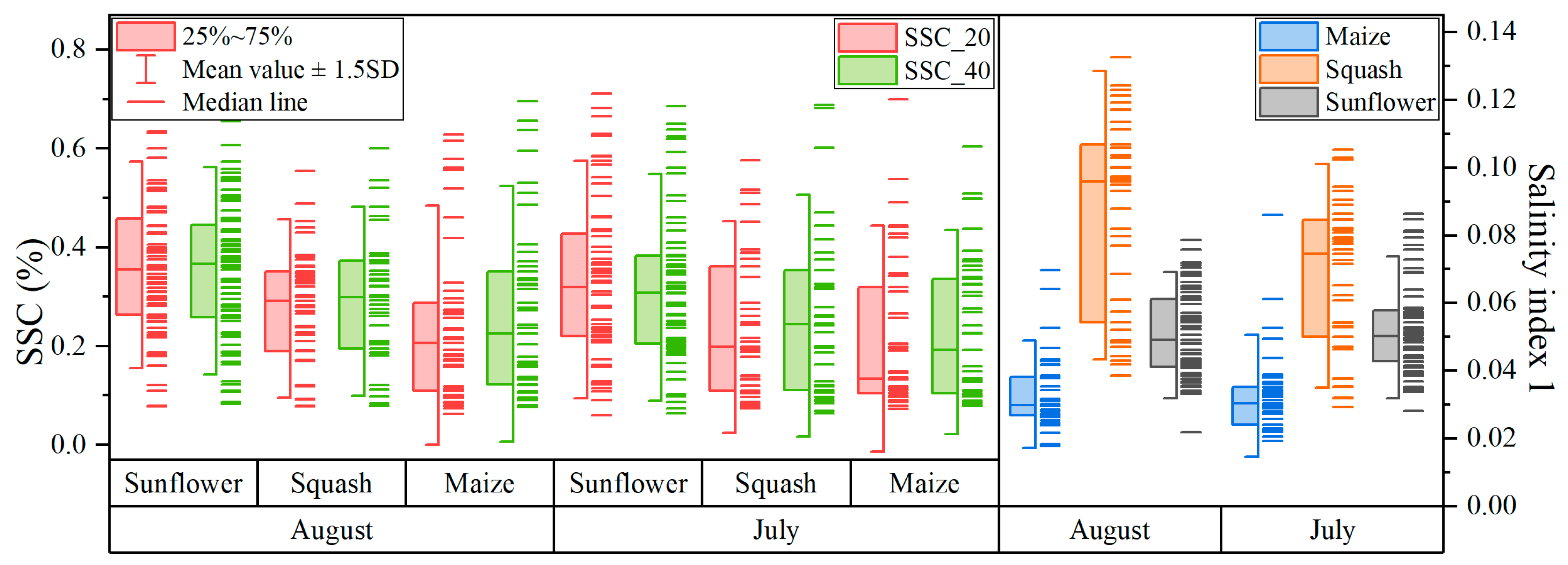
In this study, the SSC and spectral index were analyzed according to diverse time series and crop types. The distribution and statistical characteristics of the data are displayed in Figure 5. The box on the left of each group of data in the figure represents the statistical characteristics of the data, and the horizontal line on the right represents data distribution density. According to the figure, the soil salinization degree in fields planted with sunflower was higher than those with maize and squash, which were concentrated in areas with mild and moderate salinization levels. The degree of soil salinization in August was slightly higher than that in July. Considering SI1 as an example, the difference between the spectral index of three crops was obvious. The SI1 of maize was the most widely distributed at approximately 0.03, whereas those of sunflower and squash were approximately 0.04 and 0.07, respectively. The difference degree of the spectral index was considerably higher than the difference degree of the SSC level of the three crops, which indicated that the spectral indices of diverse crops may respond differently to SSC. The SI1 of the same crop also fluctuated to a certain extent in diverse time sequences.
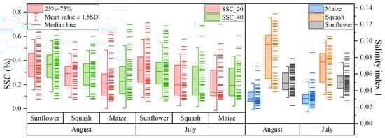
Figure 5.
Box plots showing SSC and SI1 statistics of various crop type and time series datasets: the horizontal line represents the data density.
3.3. Response Analysis of the Spectral Index to SSC
In this study, the response of SSC and the spectral index under diverse crop types and time series were analyzed based on the PCC method. The r-value results for each dataset are displayed using the heatmap representation (Figure 6). In this figure, it can be seen that the correlations between the SSC in the 0–20 cm depth and most spectral indices are stronger than those in the 20–40 cm range. Thus, the SSC in 0–20 cm depth is more sensitive to the spectral index response. The dataset was divided into July and August for analysis (Figure 6b). Compared with the dataset for the undivided months, the r-values of most spectral indices increased slightly in July (the highest r-value increase was 0.09). In August, the r-value was slightly lower (the highest r-value reduction was −0.12), which could be related to the longer data collection period in August. By contrast, when the dataset was divided into different crop types, the correlation between almost all spectral indices and the SSC increased to varying degrees (Figure 6c). For example, the r-values of SI1 and SI9 of squash increased by 0.26 and 0.27, respectively. This phenomenon confirmed the results in Section 3.2, whereby the spectral indices of various crop types have distinct responses to SSC and the classification of crop types can effectively improve the correlation between spectral independent and SSC-dependent variables.
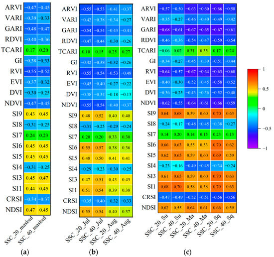
Figure 6.
Heatmap showing the r-values of various datasets: (a) original dataset after mask; (b) dataset divided into different time series; (c) dataset divided into different crop type; Jul stands for July; Aug stands for August; Su stands for sunflower; Ma stands for maize; Sq stands for squash.
To investigate whether a cumulative effect occurs between SSC and the spectral index in different time series and crop types, the datasets were subdivided according to these two factors for correlation analysis (Figure 7). When simultaneously dividing by crop type and time series, we found that the correlation between SSC and the spectral index was improved to a certain extent on the basis of only dividing by crop type. For example, the r-values between SSC in 0–20 cm depth and NDSI, NDVI, GARI, etc., in maize fields in August were all higher than 0.8. The response degree of the spectral index to SSC could be improved by time series division on the basis of crop classification.
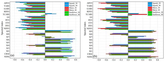
Figure 7.
Correlation coefficient (r) between SSC and spectral indices in different crop types and time series; (a) correlation coefficient (r) for each crop type in July; (b) correlation coefficient (r) for each crop type in August.
3.4. SSC Modeling Using Machine Learning Methods
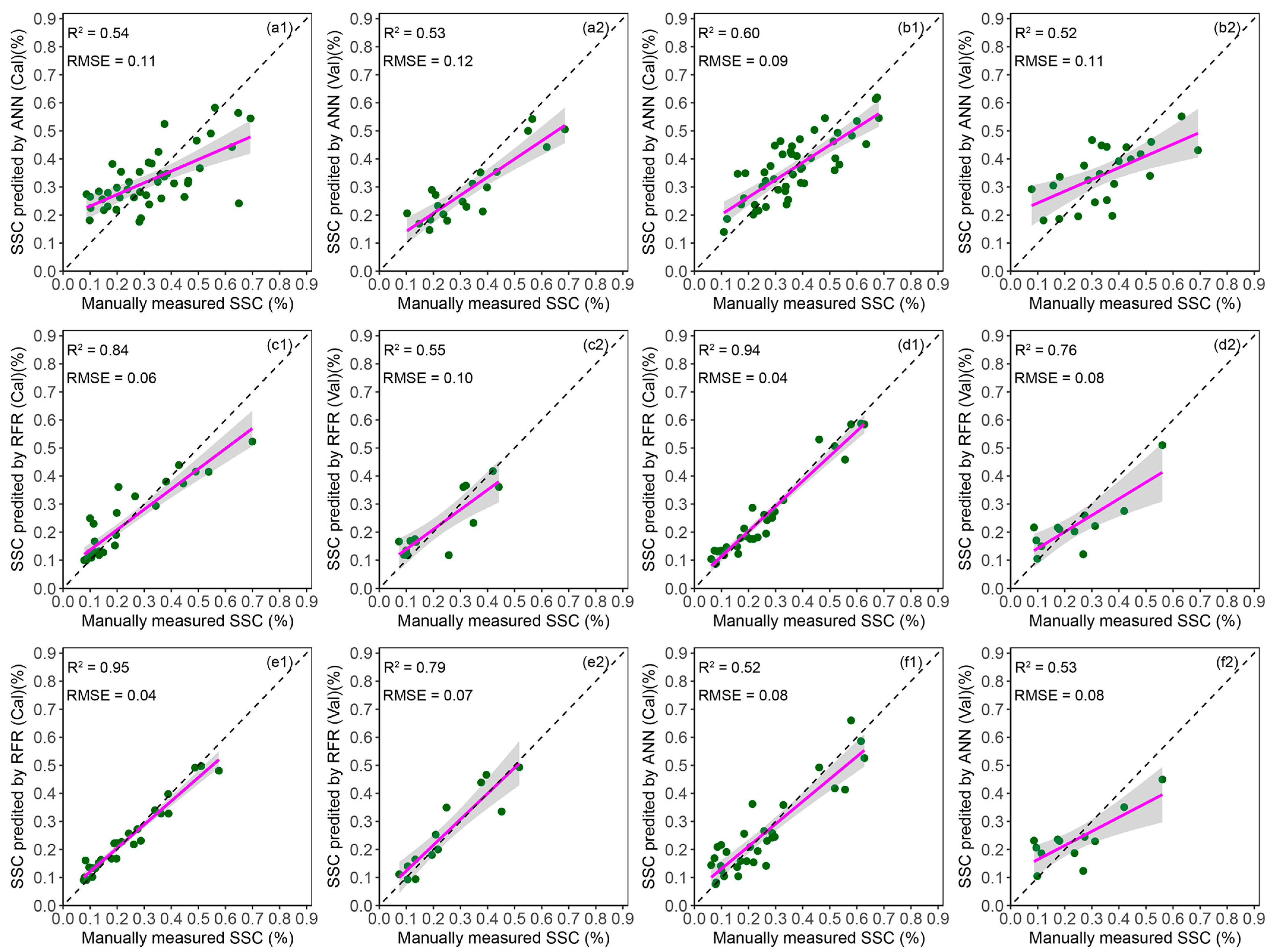
In order to confirm whether these two environmental factors can promote modeling accuracy, the spectral indices of the top 5 r-values of the above datasets were considered as modeling parameters (Table 3), and three machine learning algorithms were used to establish estimation models for these six datasets. Figure 8 displays the model performance parameters. The results of validation datasets were used as evaluation indices of model performance. The results are basically consistent with those described in Section 3.3. The separate division of different time series or crop types improved the accuracy of SSC in 0–20 cm depth estimation models but did not have a positive effect on partial 20–40 cm datasets. The datasets were divided into six sub-datasets, namely, sunflower_July, sunflower_August, maize_July, maize_August, squash_July, and squash_August, and the three machine learning algorithms were used for modeling. Table 4 presents the model parameters and results. The results revealed that the performance of the model was greatly improved by the simultaneous classification of crop types and time series (R2 = 0.52–0.79, RMSE = 0.07–0.12%, LCCC = 0.77–0.92, RPD = 1.60–2.60). The RFR and ANN algorithms were superior to the SVR algorithm, and both of the algorithms had the better performance in the modeling of different datasets. The ANN was more stable than the RFR in terms of model generalization ability, and the accuracy of the calibration dataset of RFR was typically higher than that of the validation dataset. With the exception of the sunflower_July dataset, the best estimated depth of the remaining datasets was 0–20 cm. The performances of models established based on the three sub-datasets in July are better than those using data from August. The RPD was close to 2 and the LCCC was greater than 0.8, which indicated that the model was predictable and that the predicted value was in good agreement with the measured value. The predictive performance of the sunflower and maize datasets in August was slightly worse, with LCCC of 0.78 and 0.77 and RPD of 1.60 and 1.76, respectively. Figure 9 shows the scatterplots of the SSC estimation and ground-truth values for the optimal models established for each crop type and time series. These plots reveal slight underestimations for severe salinization data. In general, the ANN and RFR were suitable algorithms for SSC estimation during the vegetation cover period.
Table 3.
The combination of characteristic variables used for modeling of each dataset.
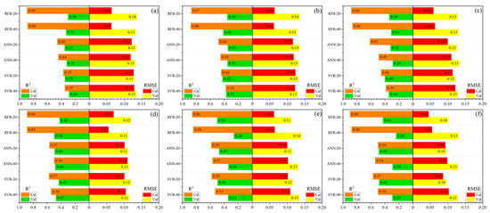
Figure 8.
Model performance parameters of different datasets: (a) entire dataset; (b) July dataset; (c) August dataset; (d) sunflower dataset; (e) maize dataset; (f) squash dataset.
Table 4.
Model performance parameters of different crop types and time series established by RFR, ANN and SVR. The best models were shown in bold.
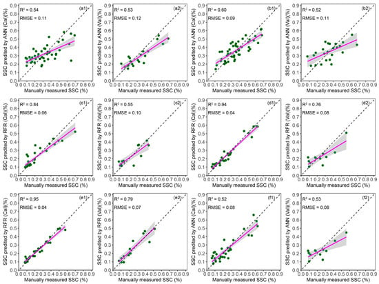
Figure 9.
The optimal model performance for different crop type and time series. The confidence interval (shaded in gray) was set to 95%. (a1) calibration dataset of sunflower_July; (a2) validation dataset of sunflower_July; (b1) calibration dataset of sunflower_August; (b2) validation dataset of sunflower_August; (c1) calibration dataset of maize_July; (c2) validation dataset of maize_July; (d1) calibration dataset of maize_August; (d2) validation dataset of maize_August; (e1) calibration dataset of squash_July; (e2) validation dataset of squash_July; (f1) calibration dataset of squash_August; (f2) validation dataset of squash_August.
3.5. Mapping Spatial Distribution of SSC
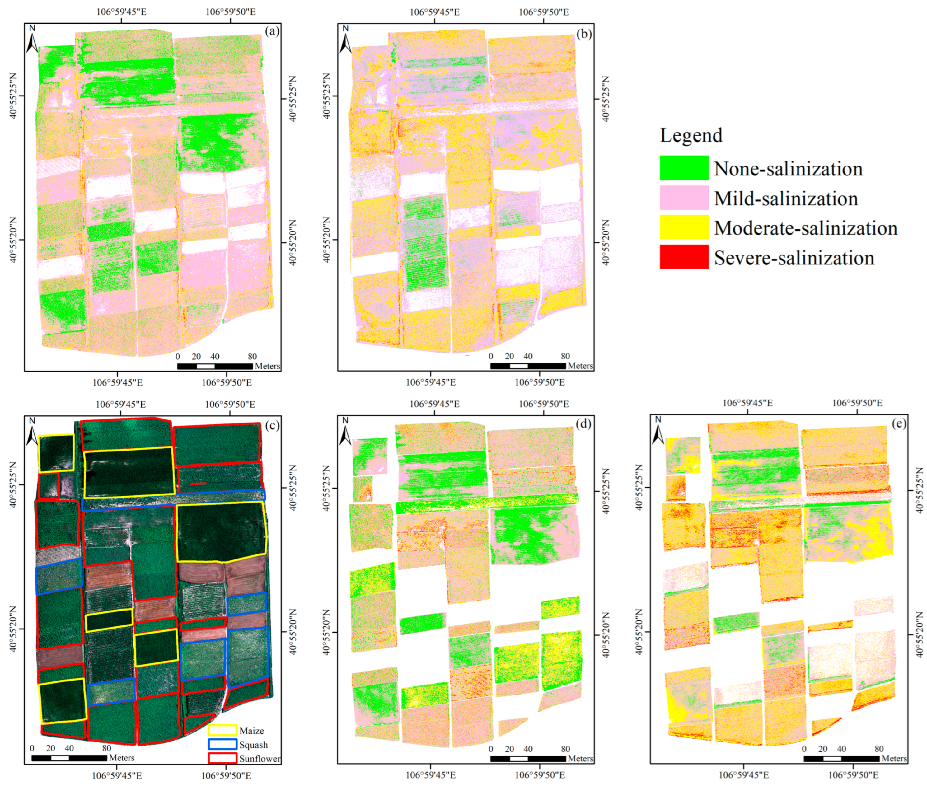
Based on the optimal estimation model under diverse environmental factors and UAV imagery, prediction distribution maps of SSC were generated. Figure 10 (study area 2 as an example) shows the predicted distribution of SSC for different periods and treatments. Different colors represent different levels of soil salinization, and the specific color meanings are given in the legend. This legend is used for all distribution maps in the figure, and the white pixels are the removed soil pixels and fields that are not the subject of this study. When generating the SSC distribution map, the independent variable spectral index distribution map of the study area should be obtained at first. Spectral indices were obtained via the band operation of the single-band multispectral image using R language. The pixels of different crop types were classified using the ground-truth value and manual calibration method. Figure 10a,b present the distribution maps for July and August using the model that did not divide crop type and time series. Figure 10d,e display the synthesized maps using multiple models categorized into different crop types and time series. The comparison of the four figures reveals that the soil salinization gradient of Figure 10d,e was more obvious, and Figure 10a,b reveal an underestimation of some sunflower fields. The prediction maps of squash fields reveal an obvious uniformity without the division of crop type and time series. Importantly, pixels of mild salinization accounts were observed. The SSC statistics of the squash sampling plots in Figure 5 reveal that the horizontal span of salinization for squash fields was large. Furthermore, the soil salinization degree in August was higher than that in July, which was consistent with our statistical situation of the ground-truth value and field observation. Therefore, the prediction distribution map of SSC based on the classification of crop types and time series achieved higher accuracy.
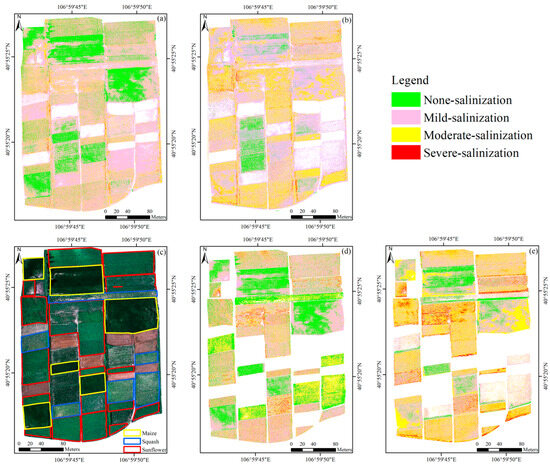
Figure 10.
Prediction maps of SSC for July and August: (a,b) are prediction maps in July and August using the model based on the entire dataset; (c) ground truth of the crop type; (d,e) prediction map in July and August using the model based on the dataset divided into different crop types and time series.
4. Discussion
4.1. Necessity of Masking Soil Pixels
Multispectral imaging technology based on spectroscopy and imaging can capture the spectral information of an object surface [48]. However, this technology cannot penetrate the crop layer to directly obtain soil surface information during the vegetation cover period. Therefore, the essence of estimating SSC during the vegetation cover period is to obtain SSC information indirectly through the response of the crop canopy spectral characteristics to SSC. The FVC of diverse crops at different growth periods is distinct, which results in the acquisition of UAV multispectral images that contain not only crop canopy spectral information, but also some soil pixel spectral information. The calculation method of the spectral index of each sampling plot involves obtaining the mean value within a unit area. Therefore, when soil pixels exist within the sampling plot range, the spectral reflectance value is affected. When the number of soil pixels between different sampling points is inconsistent, the correlations between spectral indices and SSC are affected. Some scholars [41] have considered the influence of soil pixels and removed it when inverting crop phenotypic and soil parameters. In this study, the PCCs between 20 spectral indices (derived from masked soil pixel images and original images) and SSC were compared. The results revealed that for the SSC 0–20 cm in depth, mask treatment only improved the r-values of 9 spectral indices and the other 11 indices had high correlation when they were unmasked. Combined with the field investigation results, this phenomenon may be attributed to the inhibition of crop growth in plots with high soil salinization levels (the leaves are typically small, and the plants are short). Therefore, the FVC of the same crop during the same period may be related to the degree of soil salinization. At this stage, the soil exposure (number of pixels) is no longer redundant information. Zhang et al. [8] estimated SSC under different FVC levels and revealed that the statistical results of measured SSC values of the same FVC level indicated that the soil salinization level of bare land with mid to low FVC levels was considerably higher than that obtained with mid to high FVC levels. After deleting spectral indices with no obvious correlation with SSC from the results in Figure 4, we revealed that, for the spectral indices with r-value > 0.4, mask processing had a positive effect on most indices. Therefore, soil pixels were finally masked. In the future, regardless of whether it is necessary to mask the soil pixels, the relationship between FVC and SSC should be meticulously studied to determine whether the soil spectral characteristic information contributes to SSC. Therefore, shielding soil pixels is necessary.
4.2. Significance of Crop Type and Time Series Division
In this study, the response degree of spectral indices to SSC as well as the modeling and mapping accuracy were improved by simultaneously classifying crop types and time series. From the perspective of the crop type, when the SSC was indirectly estimated by the spectral reflectance of vegetation canopy, the canopy structure characteristics of crops are critical and directly affect the canopy spectral characteristics. The differences in canopy phenotypic characteristics among different crop types are closely related to growth physiological characteristics of crops [22], whereas the differences in canopy spectral characteristics of the same crop may be related to different degrees of soil salinization. The results in Figure 5 revealed that the intervals of the spectral index values of the three crops differ considerably. The SSC of the three crops also revealed the order of sunflower > squash > maize, which was related to the saline–alkaline tolerance of the crops. Therefore, the simple division of datasets according to diverse crop types improved the correlations between the spectral indices, SSC, and modeling accuracy. From the perspective of different time series, crops have distinct canopy characteristics in diverse growth stages. Maize is in the heading stage in July and the milky maturity stage in August, whereas sunflower is in the squaring stage in July and the blooming stage in August. Squash began to enter the knot melon stage in late July, and most leaves reached senescence by late August [20]. The changes in canopy phenotypic characteristics caused the different spectral characteristics of the three crops at different time series. Therefore, dividing different time series based on crop classification strengthens the correlation between spectral variables and SSC, with a maximum increase of 0.348 in the r-value (GARI of size in August).
4.3. Estimation Models of SSC
In previous studies, the superiority of machine learning methods in estimating SSC was demonstrated by the complex nonlinear and indirect relationships between variables [8,22]. In this study, RFR, ANN, and SVR were used to model SSC in different crop types and time series. According to the results of model evaluation indicators, RFR and ANN have more advantages in estimating SSC during the vegetation cover period. Although SVM has a strong generalization ability that allows it to deal with nonlinear problems, it is sensitive to noisy data [49]. However, a small quantity of severe salinization data was used in the study, which may have affected the fitting accuracy of the SVM model. Although RFR achieved higher training accuracy, an overfitting phenomenon occurred, which resulted in considerable differences in terms of accuracy between the validation and calibration datasets. ANN achieved the best performance in model stability and generalization ability, and the model precision was high. The modeling results revealed that the performance and accuracy of the model were improved considerably by dividing crop types and time series, and the R2 of the model increased by 0.17–0.44. However, certain problems, such as the increase in the number of models, reduced the feasibility of using the model in practical applications. Therefore, the time series should be first judged and the data of different crop types should be divided. Future studies should consider how to directly participate in modeling using factors such as crop type as covariates in the model. Furthermore, other influencing factors that affect crop canopy parameters, such as water stress, were confirmed in previous studies to affect SSC estimation results [41]. Therefore, considering more crops and environmental factors has a positive significance in improving model accuracy.
4.4. Prediction Maps of SSC
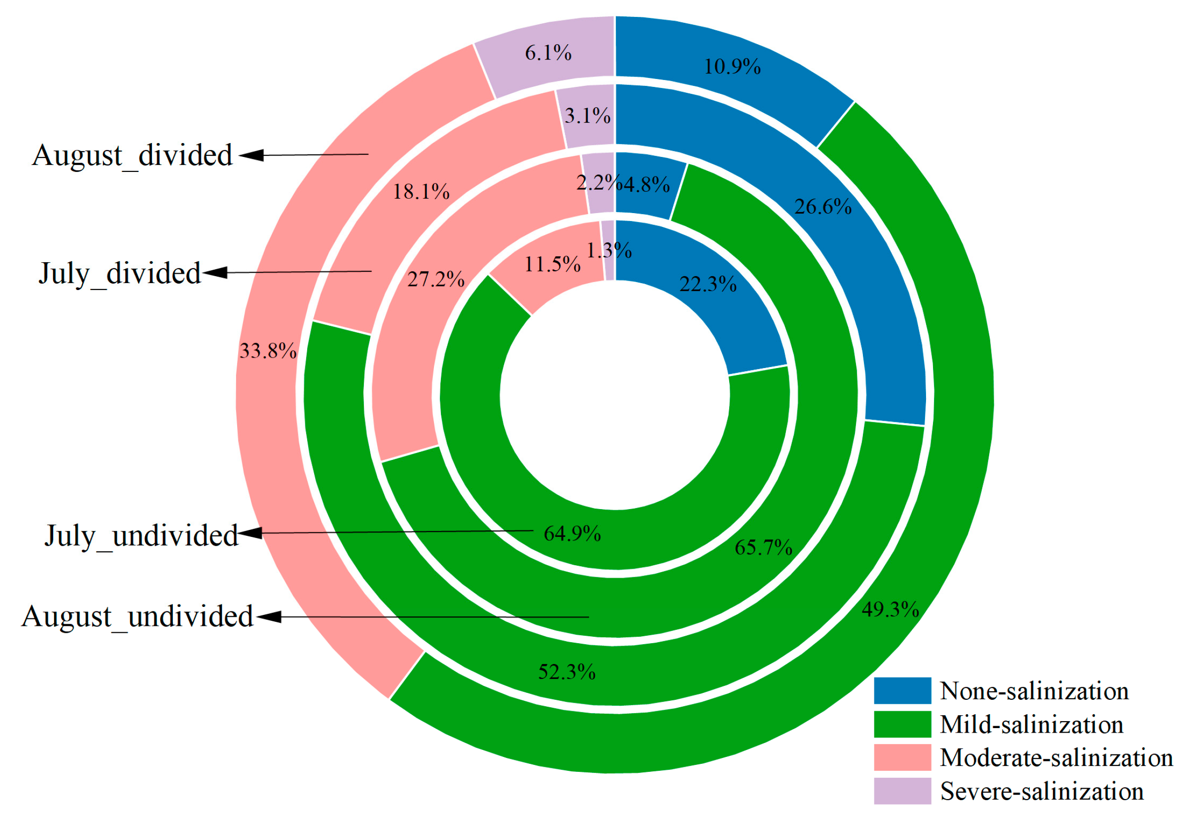
In this study, different crop fields in UAV images were divided according to the ground-truth data of crop types. After clipping the pixels of different crops, SSC estimation was performed based on the optimal model of each part and the results were subsequently combined to obtain SSC spatial prediction maps with higher accuracy. Statistical analyses of pixel percentages of various salinization degrees were performed on the SSC prediction maps for July and August (Figure 11). The statistical results revealed that, compared with July, the soil salinization degree in August considerably reduced the quantity of no salinization pixels, increased the quantity of moderately salinized pixels, and enhanced the overall salinization degree. This phenomenon could be related to irrigation. In mid to late August, squash matures and its leaves wilt. Furthermore, maize and sunflower are also in the mature stage by this time. During this period, squash field irrigation has stopped, and fields planted with other crops also considerably reduce irrigation. Therefore, the salt in soil migrated vertically to the soil surface with evaporation, which resulted in a large accumulation of salt in the soil surface (0–20 cm). It can be seen from the proportion of pixels for various salinization levels that prediction maps divided by crop type and time series were closer to displaying the proportion of ground truth (Table 2) than the undivided maps. This result proved that SSC prediction maps divided by environmental factors achieved higher accuracy than others. However, when a monitoring area contains other crops, the SSC distribution of that crop should be modeled and mapped separately. Further studies are required to analyze crop responses to SSC using smarter crop type identification methods.

Figure 11.
The pixel statistics of different salinization levels for different periods and treatments.
5. Conclusions
In this study, the effects of diverse crop types and time series on the estimation accuracy of SSC at diverse soil depths were discussed. An estimation model was established and prediction maps were generated. The results revealed the following conclusions: the sensitivity response of the spectral index variables to SSC was improved by simultaneously dividing crop types and time series, and the accuracy of modeling and mapping was improved considerably; the estimation performance of surface soil (0–20 cm) based on a UAV-derived spectrum was higher than that of deep soil (20–40 cm); masking soil pixels can improve the response degree of some spectral indices to SSC; and both RFR and ANN regression algorithms are suitable for modeling SSC during the vegetation cover period, with the model established by ANN exhibiting better generalization ability. There are also some limitations in the study: when the study area contains crops other than sunflower, maize and squash, the response of crops to SSC has not been studied, resulting in an inability to obtain the spatial distribution of SSC for the field with other crops. Additionally, the division of crop types and time series improves the accuracy of the model, but the use of multiple models also increases the application difficulty. In the future, researchers should consider including environmental factors in the modeling as covariates in order to reduce the number of models.
Author Contributions
Conceptualization, X.C. and W.H.; data curation, X.C., Y.D., W.M. and S.H.; formal analysis, X.C. and W.M.; investigation, X.C., W.M., S.H. and X.Z.; writing—original draft, X.C.; writing—review and editing, W.H. and L.Z. All authors have read and agreed to the published version of the manuscript.
Funding
This study was supported by the National Natural Science Foundation of China [51979233], the Shaanxi Province Key Research and Development Projects [2023-YBNY-221] and [2022KW-47].
Data Availability Statement
Not applicable.
Acknowledgments
We are grateful to Jiawei Cui, Jianyi Ao for data collection, and we also appreciate for Cunwang Jin, Junxiao Miao in Green Industry Development Center of Wuyuan County for providing experimental conditions.
Conflicts of Interest
The authors declare no conflict of interest.
References
- Singh, A. Soil salinity: A global threat to sustainable development. Soil Use Manag. 2022, 38, 39–67. [Google Scholar] [CrossRef]
- Sun, Y.; Li, X.; Shi, H.; Cui, J.; Wang, W.; Ma, H.; Chen, N. Modeling salinized wasteland using remote sensing with the integration of decision tree and multiple validation approaches in Hetao irrigation district of China. Catena 2022, 209, 105854. [Google Scholar] [CrossRef]
- Ivushkin, K.; Bartholomeus, H.; Bregt, A.K.; Pulatov, A.; Franceschini, M.H.D.; Kramer, H.; van Loo, E.N.; Jaramillo Roman, V.; Finkers, R. UAV based soil salinity assessment of cropland. Geoderma 2019, 338, 502–512. [Google Scholar] [CrossRef]
- Wei, G.; Li, Y.; Zhang, Z.; Chen, Y.; Chen, J.; Yao, Z.; Lao, C.; Chen, H. Estimation of soil salt content by combining UAV-borne multispectral sensor and machine learning algorithms. PeerJ 2020, 8, e9087. [Google Scholar] [CrossRef]
- Zhu, C.; Ding, J.; Zhang, Z.; Wang, Z. Exploring the potential of UAV hyperspectral image for estimating soil salinity: Effects of optimal band combination algorithm and random forest. Spectrochim. Acta A Mol. Biomol. Spectrosc. 2022, 279, 121416. [Google Scholar] [CrossRef] [PubMed]
- Lu, J.; Eitel, J.U.H.; Engels, M.; Zhu, J.; Ma, Y.; Liao, F.; Zheng, H.; Wang, X.; Yao, X.; Cheng, T.; et al. Improving Unmanned Aerial Vehicle (UAV) remote sensing of rice plant potassium accumulation by fusing spectral and textural information. Int. J. Appl. Earth Obs. 2021, 104, 102592. [Google Scholar] [CrossRef]
- Tang, Y.; Ma, J.; Xu, J.; Wu, W.; Wang, Y.; Guo, H. Assessing the Impacts of Tidal Creeks on the Spatial Patterns of Coastal Salt Marsh Vegetation and Its Aboveground Biomass. Remote Sens. 2022, 14, 1839. [Google Scholar] [CrossRef]
- Zhang, J.; Zhang, Z.; Chen, J.; Chen, H.; Jin, J.; Han, J.; Wang, X.; Song, Z.; Wei, G. Estimating soil salinity with different fractional vegetation cover using remote sensing. Land Degrad. Dev. 2021, 32, 597–612. [Google Scholar] [CrossRef]
- Yang, L.; Huang, C.; Liu, G.; Liu, J.; Zhu, A. Mapping Soil Salinity Using a Similarity-based Prediction Approach: A Case Study in Huanghe River Delta, China. Chin. Geogr. Sci. 2015, 25, 283–294. [Google Scholar] [CrossRef]
- Scudiero, E.; Skaggs, T.H.; Corwin, D.L. Regional-scale soil salinity assessment using Landsat ETM+ canopy reflectance. Remote Sens. Environ. 2015, 169, 335–343. [Google Scholar] [CrossRef]
- Ivushkin, K.; Bartholomeus, H.; Bregt, A.K.; Pulatov, A.; Bui, E.N.; Wilford, J. Soil salinity assessment through satellite thermography for different irrigated and rainfed crops. Int. J. Appl. Earth Obs. 2018, 68, 230–237. [Google Scholar] [CrossRef]
- Li, Y.; Chang, C.; Wang, Z.; Zhao, G. Remote sensing prediction and characteristic analysis of cultivated land salinization in different seasons and multiple soil layers in the coastal area. Int. J. Appl. Earth Obs. 2022, 111, 102838. [Google Scholar] [CrossRef]
- Wang, N.; Xue, J.; Peng, J.; Biswas, A.; He, Y.; Shi, Z. Integrating Remote Sensing and Landscape Characteristics to Estimate Soil Salinity Using Machine Learning Methods: A Case Study from Southern Xinjiang, China. Remote Sens. 2020, 12, 4118. [Google Scholar] [CrossRef]
- Poblete, T.; Ortega-Farías, S.; Moreno, M.A.; Bardeen, M. Artificial Neural Network to Predict Vine Water Status Spatial Variability Using Multispectral Information Obtained from an Unmanned Aerial Vehicle (UAV). Sensors 2017, 17, 2488. [Google Scholar] [CrossRef]
- Phonphan, W.; Tripathi, N.K.; Tipdecho, T.; Eiumnoh, A. Modelling electrical conductivity of soil from backscattering coefficient of microwave remotely sensed data using artificial neural network. Geocarto Int. 2014, 29, 842–859. [Google Scholar] [CrossRef]
- Jiang, H.; Rusuli, Y.; Amuti, T.; He, Q. Quantitative assessment of soil salinity using multi-source remote sensing data based on the support vector machine and artificial neural network. Int. J. Remote Sens. 2018, 40, 284–306. [Google Scholar] [CrossRef]
- Qi, G.; Zhao, G.; Xi, X. Soil Salinity Inversion of Winter Wheat Areas Based on Satellite-Unmanned Aerial Vehicle-Ground Collaborative System in Coastal of the Yellow River Delta. Sensors 2020, 20, 6521. [Google Scholar] [CrossRef]
- Cao, Z.; Zhu, T.; Cai, X. Hydro-agro-economic optimization for irrigated farming in an arid region: The Hetao Irrigation District, Inner Mongolia. Agric. Water Manage. 2023, 277, 108095. [Google Scholar] [CrossRef]
- Li, D.; Zhang, J.; Wang, G.; Wang, X.; Wu, J. Impact of changes in water management on hydrology and environment: A case study in North China. J. Hydro-Environ. Res. 2020, 28, 75–84. [Google Scholar] [CrossRef]
- Li, G.; Han, W.; Dong, Y.; Zhai, X.; Huang, S.; Ma, W.; Cui, X.; Wang, Y. Multi-Year Crop Type Mapping Using Sentinel-2 Imagery and Deep Semantic Segmentation Algorithm in the Hetao Irrigation District in China. Remote Sens. 2023, 15, 875. [Google Scholar] [CrossRef]
- Zhang, L.; Niu, Y.; Zhang, H.; Han, W.; Li, G.; Tang, J.; Peng, X. Maize Canopy Temperature Extracted from UAV Thermal and RGB Imagery and Its Application in Water Stress Monitoring. Front. Plant Sci. 2019, 10, 1270. [Google Scholar] [CrossRef]
- Cui, X.; Han, W.; Zhang, H.; Cui, J.; Ma, W.; Zhang, L.; Li, G. Estimating soil salinity under sunflower cover in the Hetao Irrigation District based on unmanned aerial vehicle remote sensing. Land Degrad. Dev. 2023, 34, 84–97. [Google Scholar] [CrossRef]
- Wang, J.; Ding, J.; Yu, D.; Ma, X.; Zhang, Z.; Ge, X.; Teng, D.; Li, X.; Liang, J.; Lizaga, I.; et al. Capability of Sentinel-2 MSI data for monitoring and mapping of soil salinity in dry and wet seasons in the Ebinur Lake region, Xinjiang, China. Geoderma 2019, 353, 172–187. [Google Scholar] [CrossRef]
- Wang, D.; Chen, H.; Wang, Z.; Ma, Y. Inversion of soil salinity according to different salinization grades using multi-source remote sensing. Geocarto Int. 2022, 37, 1274–1293. [Google Scholar] [CrossRef]
- Scudiero, E.; Skaggs, T.H.; Corwin, D.L. Regional scale soil salinity evaluation using Landsat 7, western San Joaquin Valley, California, USA. Geoderma Regional. 2014, 2–3, 82–90. [Google Scholar] [CrossRef]
- Ding, J.; Yu, D. Monitoring and evaluating spatial variability of soil salinity in dry and wet seasons in the Werigan–Kuqa Oasis, China, using remote sensing and electromagnetic induction instruments. Geoderma 2014, 235–236, 316–322. [Google Scholar] [CrossRef]
- Douaoui, A.E.K.; Nicolas, H.; Walter, C. Detecting salinity hazards within a semiarid context by means of combining soil and remote-sensing data. Geoderma 2006, 134, 217–230. [Google Scholar] [CrossRef]
- Allbed, A.; Kumar, L.; Aldakheel, Y.Y. Assessing soil salinity using soil salinity and vegetation indices derived from IKONOS high-spatial resolution imageries: Applications in a date palm dominated region. Geoderma 2014, 230–231, 1–8. [Google Scholar] [CrossRef]
- Bannari, A.; Guedon, A.M.; El Harti, A.; Cherkaoui, F.Z.; El Ghmari, A. Characterization of Slightly and Moderately Saline and Sodic Soils in Irrigated Agricultural Land using Simulated Data of Advanced Land Imaging (EO-1) Sensor. Commun. Soil Sci. Plan. 2008, 39, 2795–2811. [Google Scholar] [CrossRef]
- Rouse, J.W.; Haas, R.H.; Schell, J.A.; Deering, D.W. Monitoring vegetation systems in the Great Plains with ERTS. NASA Spec. Publ. 1974, 351, 309. [Google Scholar]
- Tucker, C.J. Red and photographic infrared l, lnear combinations for monitoring vegetation. Remote Sens. Environ. 1979, 8, 127–150. [Google Scholar] [CrossRef]
- Wang, Z.X.; Liu, C.; Huete, A. From AVHRR-NDVI to MODIS-EVI: Advances in vegetation index research. Acta Ecol. Sin. 2003, 23, 979–987. [Google Scholar]
- Gao, G.; Wang, S. Compare Analysis of Vegetation Cover Change in Jianyang City Based on RVI and NDVI. In Proceedings of the 2012 2nd International Conference on Remote Sensing, Environment and Transportation Engineering, Nanjing, China, 1–3 June 2012; pp. 1–4. [Google Scholar]
- Gamon, J.A.; Surfus, J.S. Assessing leaf pigment content and activity with a reflectometer. New Phytologist. 1999, 143, 105–117. [Google Scholar] [CrossRef]
- Haboudane, D.; Miller, J.R.; Tremblay, N.; Zarco-Tejada, P.J.; Dextraze, L. Integrated narrow-band vegetation indices for prediction of crop chlorophyll content for application to precision agriculture. Remote Sens. Environ. 2002, 81, 416–426. [Google Scholar] [CrossRef]
- Roujean, J.; Breon, F. Estimating PAR absorbed by vegetation from bidirectional reflectance measurements. Remote Sens. Environ. 1995, 51, 375–384. [Google Scholar] [CrossRef]
- Gitelson, A.A.; Kaufman, Y.J.; Merzlyak, M.N. Use of a green channel in remote sensing of global vegetation from EOS-MODIS. Remote Sens. Environ. 1996, 58, 289–298. [Google Scholar] [CrossRef]
- Gitelson, A.A.; Stark, R.; Grits, U.; Rundquist, D.; Kaufman, Y.; Derry, D. Vegetation and soil lines in visible spectral space: A concept and technique for remote estimation of vegetation fraction. Int. J. Remote Sens. 2002, 23, 2537–2562. [Google Scholar] [CrossRef]
- Kaufman, Y.J.; Tanre, D. Atmospherically resistant vegetation index (ARVI) for EOS-MODIS. IEEE Trans. Geosci. Remote Sens. 1992, 30, 261–270. [Google Scholar] [CrossRef]
- Li, C.; Han, W.; Peng, M.; Zhang, M. Abiotic and biotic factors contribute to CO2 exchange variation at the hourly scale in a semiarid maize cropland. Sci. Total Environ. 2021, 784, 147170. [Google Scholar] [CrossRef]
- Zhang, L.; Han, W.; Niu, Y.; Chávez, J.L.; Shao, G.; Zhang, H. Evaluating the sensitivity of water stressed maize chlorophyll and structure based on UAV derived vegetation indices. Comput. Electron. Agric. 2021, 185, 106174. [Google Scholar] [CrossRef]
- Periasamy, S.; Ravi, K.P. A novel approach to quantify soil salinity by simulating the dielectric loss of SAR in three-dimensional density space. Remote Sens. Environ. 2020, 251, 112059. [Google Scholar] [CrossRef]
- Wang, N.; Peng, J.; Xue, J.; Zhang, X.; Huang, J.; Biswas, A.; He, Y.; Shi, Z. A framework for determining the total salt content of soil profiles using time-series Sentinel-2 images and a random forest-temporal convolution network. Geoderma 2022, 409, 115656. [Google Scholar] [CrossRef]
- Poldrack, R.A.; Huckins, G.; Varoquaux, G. Establishment of Best Practices for Evidence for Prediction: A Review. Jama Psychiat. 2020, 77, 534–540. [Google Scholar] [CrossRef] [PubMed]
- Wang, Z.; Zhang, X.; Zhang, F.; Chan, N.W.; Kung, H.; Liu, S.; Deng, L. Estimation of soil salt content using machine learning techniques based on remote-sensing fractional derivatives, a case study in the Ebinur Lake Wetland National Nature Reserve, Northwest China. Ecol. Indic. 2020, 119, 106869. [Google Scholar] [CrossRef]
- Lin, L.I. A Concordance Correlation Coefficient to Evaluate Reproducibility. Int. Biom. Soc. 1989, 1, 255–268. [Google Scholar] [CrossRef]
- Rossel, R.A.V.; Webster, R. Predicting soil properties from the Australian soil visible-near infrared spectroscopic database. Eur. J. Soil Sci. 2012, 63, 848–860. [Google Scholar] [CrossRef]
- Garini, Y.; Young, I.T.; McNamara, G. Spectral Imaging: Principles and Applications. Cytom. Part A 2006, 69A, 735–747. [Google Scholar] [CrossRef]
- Shieh, H.; Kuo, C. A reduced data set method for support vector regression. Expert Syst. Appl. 2010, 37, 7781–7787. [Google Scholar] [CrossRef]


Disclaimer/Publisher’s Note: The statements, opinions and data contained in all publications are solely those of the individual author(s) and contributor(s) and not of MDPI and/or the editor(s). MDPI and/or the editor(s) disclaim responsibility for any injury to people or property resulting from any ideas, methods, instructions or products referred to in the content. |
© 2023 by the authors. Licensee MDPI, Basel, Switzerland. This article is an open access article distributed under the terms and conditions of the Creative Commons Attribution (CC BY) license (https://creativecommons.org/licenses/by/4.0/).