Multi-Prior Graph Autoencoder with Ranking-Based Band Selection for Hyperspectral Anomaly Detection

Abstract

Hyperspectral anomaly detection (HAD) is an important technique used to identify objects with spectral irregularity that can contribute to object-based image analysis. Latterly, significant attention has been given to HAD methods based on Autoencoders (AE). Nevertheless, due to a lack of prior information, transferring of modeling capacity, and the “curse of dimensionality”, AE-based detectors still have limited performance. To address the drawbacks, we propose a Multi-Prior Graph Autoencoder (MPGAE) with ranking-based band selection for HAD. There are three main components: the ranking-based band selection component, the adaptive salient weight component, and the graph autoencoder. First, the ranking-based band selection component removes redundant spectral channels by ranking the bands by employing piecewise-smooth first. Then, the adaptive salient weight component adjusts the reconstruction ability of the AE based on the salient prior, by calculating spectral-spatial features of the local context and the multivariate normal distribution of backgrounds. Finally, to preserve the geometric structure in the latent space, the graph autoencoder detects anomalies by obtaining reconstruction errors with a superpixel segmentation-based graph regularization. In particular, the loss function utilizes ${\ell }_{2,1}-\mathrm{norm}$ and adaptive salient weight to enhance the capacity of modeling anomaly patterns. Experimental results demonstrate that the proposed MPGAE effectively outperforms other state-of-the-art HAD detectors.

1. Introduction

As opposed to visible and multispectral images, hyperspectral images (HSIs) have been regarded as a remarkable invention in the field of remote sensing imaging sciences, due to their practical capacity to capture high-dimensional spectral information from different scenes on the Earth’s surface [1]. HSIs consist of innumerable contiguous spectral bands that span the electromagnetic spectrum, providing rich and detailed physical attributes of land covers, which facilitate the development of various applications such as change detection [2,3,4,5], land-cover classification [6,7,8], retrieval [9], scene classification [10,11] and anomaly detection [12,13].

Anomaly detection aims to find abnormal patterns whose distribution is inconsistent with most instances in data [14,15]. As one significant branch of hyperspectral remote sensing target detection, hyperspectral anomaly detection (HAD) involves the unsupervised identification of targets (e.g., plastic plates in a field or military camouflage targets [16,17,18]) that exhibit spatial or spectral dissimilarities from their surrounding background without relying on prior information in practical situations [19,20]. Therefore, in essence, HAD is a binary classification with training in an unsupervised manner. Although the precise definition of an anomaly has yet to be established [21,22], it is generally accepted that HAD typically exhibits the following characteristics: (1) generally, anomalies constitute a very small proportion of the entire hyperspectral image; (2) anomalies can be distinguished from the background in terms of spectral or spatial characteristics. (3) there is a lack of spatial and spectral prior information about anomalies or anomalies; (4) in real-world situations, occasional spectral mixing of anomalies and background may appear as pixels or subpixels. These attributes render hyperspectral anomaly detection a prominent yet challenging topic in the field of remote sensing [23,24,25]. Over recent decades, numerous HAD algorithms can be broadly classified into two categories based on their motivation and theoretical basis: traditional and deep-learning-based methods.

Traditional HAD methods have two important branches: statistics- and representation-based methods. Statistics-based HAD methods generally assume that the background of the HSIs may obey some distributions, such as multivariate Gaussian distribution. In contrast, anomalous objects inconsistent with distribution can be identified based on the Mahalanobis distance or the Euclidean distance. Among these statistics-based HAD methods, the Reed-Xiaoli (RX) [26] detector, one of the most well-known benchmarks, considers the original image as the background statistics based on Gaussian multivariate distribution, and pixels exhibiting deviations from the distribution are identified as anomalies. As the neglect of local context in RX, local variants of RX (LRX) [27,28] estimate the test pixels by modeling a small neighborhood as the local background statistics. However, the two versions of RX suffer from the limitation of the fact that the real-world scene may obey the complex high-order distribution. Thus, some nonlinear variants of the RX detector, kernel RX (KRX) [29,30,31], were presented, which nonlinearly map the entire images to high-dimension feature space by different kernel functions. Since most RX-based methods ignore the spatial information, He et al. [32] developed RX with extended multi-attribute profiles in a recursive manner. In addition to the RX and its variants, several effective methods based on statistics have also been developed. As a unified approach to object and change detection, the Cluster-Based Anomaly Detection (CBAD) [33] calculates background statistics across clusters rather than sliding windows, enabling the detection of objects with varying sizes and shapes. As an important algorithm of statistical learning, the kernel isolation forest detector (KIFD) [34] and its improvement [35] have been used for HAD, which assumes the anomalies are more prone to isolation within the kernel space.

Based on the improvement of compressed sensing theory, representation-based methods can detect anomalies without certain assumptions about the background distribution. The fundamental concept of representation-based methods is that all test pixels can be reconstructed by utilizing a specific background dictionary in a logical model where the residual represents the abnormal level of the pixels. Moreover, representation-based methods include collaborative representation (CR), the sparse representation (SR), and the low-rank representation (LRR). The CR-based methods assume collaboration between dictionary atoms is more crucial than competition in small sample cases. Specifically, the background pixel can be linearly represented well by its surroundings while the objects cannot, and the representation residual is considered to be an abnormal level of the test pixels [36,37]. To improve the robustness of CR and reduce testing time, a non-negative-constrained joint collaborative representation (NJCR) [38] model has been proposed. In contrast to CR, SR focuses on the competition of atoms, it assumes that background representation can be achieved by a few atoms from an overcomplete dictionary. In the work by [39], based on a binary hypothesis, background joint sparse representation was utilized to detect anomalies. The robust background regression-based score estimation algorithm (RBRSE) [40] exploits a kernel expansion technique to formulate the information as a density feature representation to facilitate robust background estimation. Due to high spatial and spectral correlation in HSIs, background exhibits global low-rank characteristics while anomalies demonstrate sparsity owing to their low probability of occurrence and limited presence. Therefore, unlike pixel-by-pixel detection of CR and SR, LRR locates the objects by characterizing the global structure of the HSIs [41]. In order to exploit the spatial–spectral information, the adaptive low-rank transformed tensor [42] restrains the frontal slices of the transformed tensor with low-rank constraint. Because of the highly mixed phenomenon of pixels, based on low-rank decomposition, Qu et al. [43,44] obtained discriminative vectors by spectral unmixing.

Since deep-learning-based methods can obtain discrimination in the space of latent semantic features, they have emerged as a prominent area of research in recent years. To date, deep learning has tackled numerous challenging issues in the field of computer vision [45,46]. In a supervised manner, based on the convolutional neural network (CNN) and fully connected layer, Li et al. [47] explored the performance of transfer learning for HAD. Many unsupervised deep-learning-based methods introduce the autoencoders (AE) as the backbone [48]. In AE-based methods, the input layer encodes the testing pixels X into hidden layers with a lower dimension and sparsity, and then the output layer decodes features to construct the pixels $\stackrel{\sim }{X}$. The residual between X and $\stackrel{\sim }{X}$ demonstrates the detection result. For instance, based on low-rank and sparse matrix decomposition, Zhao et al. [49] developed a spectral–spatial stacked autoencoder to extract deep features. To reduce the high dimensionality and remove deteriorated spectral channels, an adversarial autoencoder [50] has been proposed, it optimized the model with an adaptive weight and spectral angle distance. Wang et al. [51] presented an autonomous AE-based HAD framework to reduce manual parameter setting and simplify the processing procedures. In [52], AE-based network to reserve geometric structure by embedding a supergraph which improved the performance. As for reducing the feature representation of the anomaly targets, guided autoencoder(GAED) [53] adopted a multilayer AE network with a guided module.

Although the representations learned by AEs benefit background estimation, there are still several problems in AE-based methods. First, most AE-style methods ignore the preprocessing of band selection. The strong spectral redundancy of HSIs may affect the performance and the excessive number of spectral bands in HSIs leads to significant computational burden [54,55]. Moreover, high-dimensional volumes may create “the curse of dimensionality”, which decreases detection accuracy [56,57]. Second, despite the recent advancements in AE-based techniques for HAD, it is important to acknowledge that the information equivalence between input and supervision in reconstruction cannot effectively force the AE to learn the required semantic features [58]. Besides, the local spatial characteristics of the HSI and the inter-pixel correlation are not explicitly considered when adopting AE to reconstruct pixels, and the lack of prior spectral and spatial information can impact the performance of HAD [52,53].

In order to address the abovementioned drawbacks, this study proposes a novel multi-prior graph autoencoder (MPGAE) for hyperspectral anomaly detection. First, inspired by PTA [59] that utilizes a piecewise-smooth prior to achieving total variation norm regularization, a novel band selection module is designed to simplify the HSIs, and it can remove redundant spectral information. Next, to balance the reconstruction of the background and anomaly targets, a new loss function is presented by combining the global RX and local salient weight based on the local salient prior. Finally, combining the new loss function and the compressed HSIs, the supergraph [52] is introduced into autoencoder to achieve the final detection.

Compared with other HAD approaches, the major contributions of the proposed MPGAE can be summarized as follows:

1

The MPGAE is proposed to handle the situations where anomalies are present in hyperspectral images. Based on the piecewise-smooth prior, the band selection module can eliminate the unnecessary spectral bands to improve the performance.

2

Based on the combination of a global RX detector and local salient weight, a new loss function is presented. The loss function can improve performance by adjusting background and anomaly feature learning.

3

The supergraph [52] is introduced into autoencoder for preserving spatial consistency and information about the local geometric structure, which can improve the robustness of the proposed MPGAE.

The experimental results utilizing five real datasets captured by various sensors, with extensive metrics, and quantitative and visual illustrations demonstrated that the proposed MPGAE method is significantly superior to the other competing methods in terms of detection accuracy.

The remainder of this article is arranged as follows. Section 2 introduces the details of the proposed method, MPGAE. Then, Section 3 discusses the experimental results of the proposed method, MPGAE, with other advanced hyperspectral anomaly detectors on five real hyperspectral datasets. Finally, Section 4 summarizes this paper and demonstrates the trends of future research.

2. Proposed Method

In this section, the proposed prior-based graph autoencoder is explored. Section 2.1 demonstrates the overview of the proposed method. Section 2.2 describes the module of band selection based on piecewise-smooth prior. Section 2.3 presents the module of adaptive weight based on salient prior. Section 2.4 explains the structure of the graph autoencoder and Section 2.5 reports the loss function.

2.1. Overview

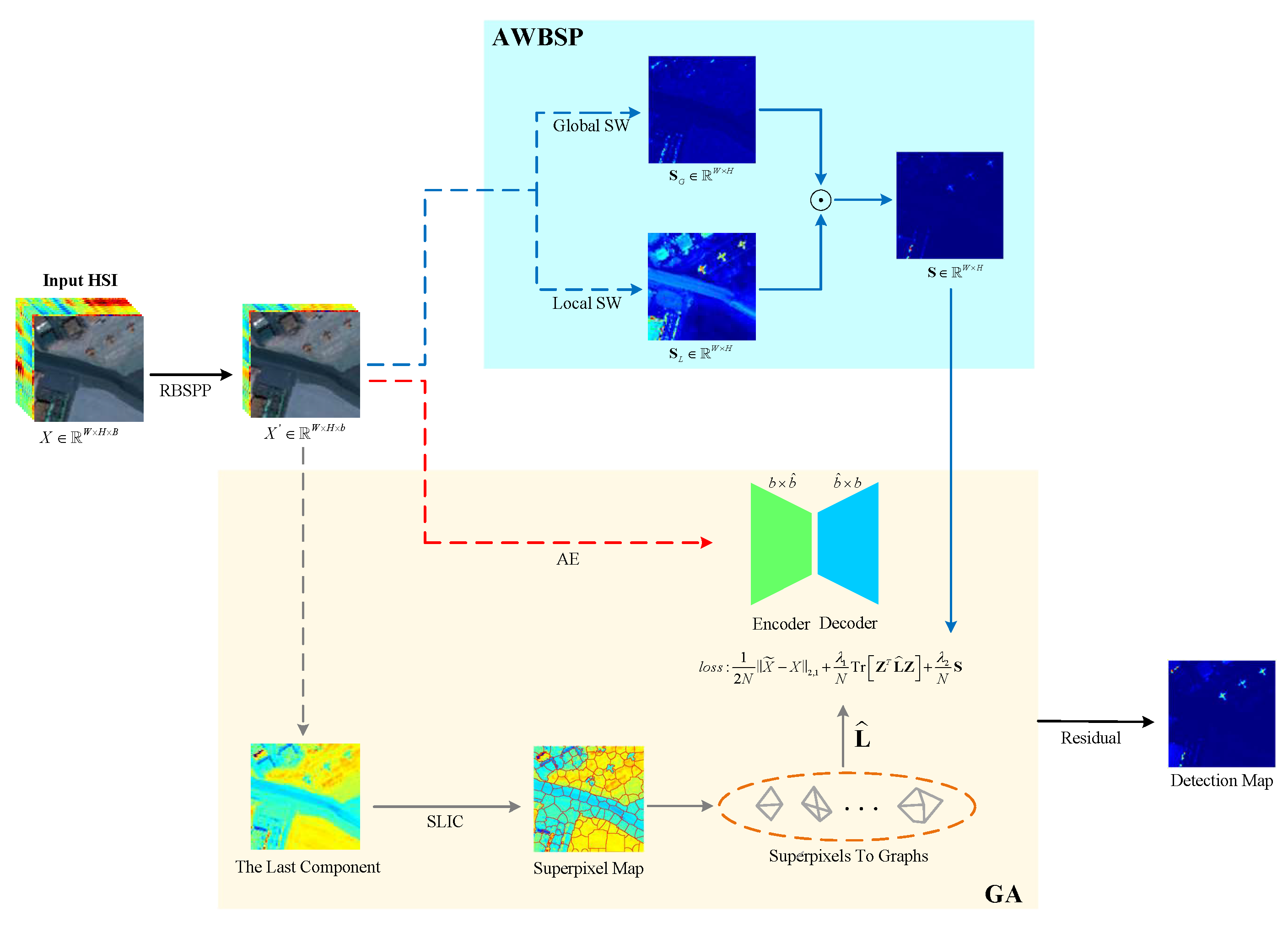
Figure 1 indicates the overall architecture of the proposed prior-based graph autoencoder. Let $X\in {\mathbb{R}}^{W\times H\times B}$ represent the input hyperspectral image where W denotes width, H denotes height, and B denotes bands. First, to reduce the spectral channels of the original hyperspectral image, a new ranking-based band selection is utilized with piecewise-smooth prior and the input becomes $X^{\prime }\in {\mathbb{R}}^{W\times H\times b}$ where b denotes the decreased bands. Next, the adaptive weight based on salient prior calculates the salient weight $S\in {\mathbb{R}}^{W\times H}$ in the global and local contexts. Meanwhile, one component of $X^{\prime }$ generates superpixels by simple linearly iterative cluster [60]. Based on the superpixels, the graphs are constructed to preserve local essential geometric information $\widehat{\mathbf{L}}$ in latent space $\mathbf{Z}$. Then, combining with ${\ell }_{2,1}$-norm, $\widehat{\mathbf{L}}$ and ${\mathbf{L}}_{SW}$, the autoencoder is trained by the loss function. Finally, the detection map is obtained by calculating the reconstruction errors. The larger the reconstruction error, the more likely the pixel represents an anomalous target.

Figure 1. The overall architecture of the proposed prior-based graph autoencoder. The proposed method mainly contains three modules: Ranking-based band selection with piecewise-smooth prior (RBSPP), adaptive weight based on salient prior (AWBSP), and graph autoencoder (GA). The AWBSP module mainly consists of local salient weight (SW) and global salient weight. SLIC means simple linearly iterative cluster.

2.2. Ranking-Based Band Selection with Piecewise-Smooth Prior

The purpose of band selection is to choose a limited number of hyperspectral bands that eliminate spectral overlap, lower computational expenses, and retain the vital spectral details of surface features. Although the backgrounds may be complex in hyperspectral images, they vary little on a finite scale, meaning each background tensor segment has a piecewise-smooth prior. Based on the observation, it can be assumed that bands with salient anomalies have large gradients that can be selected to achieve better detection performance and computational efficiency.

As mentioned above, $X\in {\mathbb{R}}^{W\times H\times B}$ denotes the original hyperspectral 3-D cube. First, all gradient values of pixels are summed for each spectral band on Euclidean distance. Since every band has only two directional variables $F=(x,y)$, the formulation can be presented as (1)

$$\begin{array}{c}{g}_k={\displaystyle \sum _{i=1}^W}{\displaystyle \sum _{j=1}^H}\{\frac{\partial F}{\partial x}\widehat{i}+\frac{\partial F}{\partial y}\widehat{j}\},\end{array}$$

(1)

where $g_k$ denotes the sum of all gradient values for k-th band. Then, the sum of gradient values are ranked for each spectral band in ascending order as follows:

$$\begin{array}{c}I=f_s\left(G\right),\end{array}$$

(2)

where $G\in {\mathbb{R}}^{1\times B}$ indicates the array of gradient value summation, $f_s$ means ascending sort function, and the index array $I\in {\mathbb{R}}^{1\times B}$ is utilized to denote the index of the elements in G along the ranked sequence. Since the substantial accumulation of gradient may obscure the difference between the anomaly and background, the module tends to preserve the spectral bands whose gradient summations are small. Namely, the smoother the corresponding grayscale image of the spectral band, the more salient the abnormal pixels. Based on compressed ratio m, after reducing the bands, the index array becomes $I^{\prime }\in {\mathbb{R}}^{1\times b}$ where $b=m\times B$ is rounded to the nearest integer. Finally, based on $I^{\prime }\in {\mathbb{R}}^{1\times b}$, X is purified to obtain $X^{\prime }\in {\mathbb{R}}^{W\times H\times b}$ where $b<B$ denotes the count of the spectral bands which are preserved in $X^{\prime }$. The formulation can be expressed as

$$\begin{array}{c}{X}^{\prime }=f_p(I^{\prime },X).\end{array}$$

(3)

2.3. Adaptive Weight Based on Salient Prior

It is widely acknowledged that anomalies can be characterized by their deviation from the background clutter and occupy a relatively small area meaningfully different from the background [61]. In other words, salient prior can be incorporated into HAD methods to improve performance.

As shown in Figure 1, a dual branch module is designed to obtain the salient weight in local and global contexts. Because the RX [26] adopts the pixels correlation matrix in a global context to detect anomalies, the RX is used to calculate the global salient weight ${\mathbf{S}}_G$ which is specified as

$$\begin{array}{c}{\mathbf{S}}_G={\left(X^{\prime }-\mu \right)}^T{\mathbf{C}}^{-1}\left(X^{\prime }-\mu \right).\end{array}$$

(4)

where $\mu$ denotes the mean vector of $X^{\prime }$ and C denotes the covariance matrix of the background distribution. The definitions of the mean vector $\mu$ and the covariance matrix C are:

$$\begin{array}{c}\begin{array}{cc}\hfill \mu & =\frac{1}{WH}{\displaystyle \sum _{i=1}^W}{\displaystyle \sum _{j=1}^H}{x}_{ij}\hfill \\ \hfill C& =\frac{1}{WH}{\displaystyle \sum _{i=1}^W}{\displaystyle \sum _{j=1}^H}\left(x_{ij}-\mu \right){\left(x_{ij}-\mu \right)}^T\hfill \end{array}\end{array}$$

(5)

where $x_{ij}$ denotes the test pixel. The W and H are the width and height of the input, respectively.

As for local salient wight $S_L$, the spectral angular distance(SAD) is utilized to obtain the adaptive saliency of every pixel. First, The SAD $S_{ij}^0$ between the mean vector $\mu$ and test pixel $x_{ij}$ is presented as

$$\begin{array}{c}{s}_{ij}^0=arccos\left(\frac{{\sum }_{m=1}^b{x}_m·{\mu }_m}{\sqrt{{\sum }_{m=1}^b{x}_m·{\sum }_{m=1}^b{\mu }_m}}\right)\end{array}$$

(6)

where b denotes the spectral bands. Then, the SAD $S_{ij}^1$ between the test pixel $x_{ij}$ and its neighborhood $y^N$ are calculated where $N=n·n-1$ is the number of surrounding pixels, the $S_{ij}^1$ is defined as

$$\begin{array}{c}{s}_{ij}^1=arccos\left(\frac{{\sum }_{m=1}^b{x}_m·y_m^n}{\sqrt{{\sum }_{m=1}^b{x}_m·{\sum }_{m=1}^b{y}_m^n}}\right)\end{array}$$

(7)

To enhance the robustness of Equation (7), the Euclidean distance between the test pixel and its local background are introduced which is expressed by

$$\begin{array}{c}{s}_{ij}^2=\left(\frac{s_{ij}^1}{\sqrt{{(i-p)}^2+{(j-q)}^2}}\right)\end{array}$$

(8)

where $(i,j)$ and $(p,q)$ indicate the position coordinates of $x_{ij}$ and $y_m^n$. Then the local salient weight $S_{ij}$ is determined as

$$\begin{array}{c}{s}_{ij}=max(s_{ij}^0,s_{ij}^2)\end{array}$$

(9)

The local salient weight of every test pixel is calculated with a sliding window which constructs the weight map for $X^{\prime }$. The final adaptive weight S based on the salient prior can be achieved as

$$\begin{array}{c}\mathbf{S}={\mathbf{S}}_G·{\mathbf{S}}_L\end{array}$$

(10)

2.4. Graph Autoencoder

In addition to the prior of piecewise smoothness and saliency, the geometric structure and local spatial information of ground objects also need to be explored. As for a hyperspectral image, superpixels are often considered to be the homogeneous parts of the individual land-cover regions [62]. Therefore, the over-segmentation procedure can be integrated into HAD methods to obtain the geometric features and local spatial context. Moreover, since superpixel segmentation algorithms are designed to reduce the complexity of images from a mess of pixels to hundreds of superpixels by grouping neighboring pixels into the same attributes that can decrease the computational complexity.

Specifically, the last component of $X^{\prime }$ is segmented into $\mathcal{P}={\left\{P_h\right\}}_{h=1}^H$ nonoverlapping same patches (superpixels) by appling SLIC [60]. Then, based on the supergraph [52] and graph regularization [63], the adjacency matrix $\mathbf{M}$ is established by sample pairs $({\mathbf{x}}_i,{\mathbf{x}}_j)$ within the same superpixels $P_h$ which are prone to belong to similar spatial and spectral domain. The similarity is measured by

$$\begin{array}{c}{m}_{ij}=exp\left(-\frac{{∥{\mathbf{x}}_i-{\mathbf{x}}_j∥}_2^2}{{\sigma }^2}\right)\end{array}$$

(11)

where $\sigma$ denotes a scalar parameter. When pixels belong to different superpixels, the $m_{ij}=0$. Then, the constraint is presented as

$${\displaystyle \underset{\mathbf{Z}}{min}}\frac{1}{2\stackrel{\sim }{N}}{\displaystyle \sum _{i=1}^{\stackrel{\sim }{N}}}{\displaystyle \sum _{j=1}^N}{m}_{ij}{∥{\mathbf{z}}_i-{\mathbf{z}}_j∥}_2^2={\displaystyle \underset{\mathbf{Z}}{min}}\frac{1}{\stackrel{\sim }{N}}Tr\left[{\mathbf{Z}}^T\mathbf{L}\mathbf{Z}\right]$$

(12)

where $\stackrel{\sim }{N}=W\times H$ denotes the number of pixels and ${\mathbf{z}}_j$ denotes the i-th column of latent space $\mathbf{Z}$. And $\mathbf{L}$ is a modified graph Laplacian matrix which is determined as

$$\mathbf{L}=\mathbf{D}-\mathbf{W}$$

(13)

where the diagonal matrix $\mathbf{D}$ denotes the degree matrix. The i-th diagonal entry $d_{ii}$ of $\mathbf{D}$ represents the degree of the i-th pixel which is formulated as

$$d_{ii}={\displaystyle \sum _{j=1}^{\stackrel{\sim }{N}}}{w}_{ij}$$

(14)

Obviously, to minimize Equation (12), the distance of $({\mathbf{z}}_i,{\mathbf{z}}_j)$ is encouraged to be small which means pixels within the same semantic superpixel can share similar representations. As for the backbone, a single-layer autoencoder is utilized which can avoid overfitting. The kernel size of convolution is $1\times 1$ with stride = 1 which can achieve dimension reductionality. Concretely, the dimensionality of the input and the output layer are both b, and the dimensionality of hidden layer $\widehat{b}$ is determined by $r\times B$ where r is a decimal between 0 and 1. And the sigmoid function is used to introduce non-linear activation into the network which can improve the representation.

2.5. Loss Function

The loss function $\mathcal{L}$ of the proposed method is defined as Equation (15), which mainly contains three terms.

$$\mathcal{L}=\frac{1}{2\stackrel{\sim }{N}}{∥\stackrel{\sim }{X}-X∥}_{2,1}+\frac{{\lambda }_1}{\stackrel{\sim }{N}}Tr\left[{\mathbf{Z}}^T\widehat{\mathbf{L}}\mathbf{Z}\right]+\frac{{\lambda }_2}{\stackrel{\sim }{N}}\mathbf{S}$$

(15)

The first term denotes the residual between hyperspectral images (HSIs) of input X and output $\stackrel{\sim }{X}$. Based on the reconstruction errors, AE can detect abnormal pixels. The higher the residual level, the greater the probability that the pixel is an anomalous target. The second term is graph regularization which can preserve local information of geometric structure in latent space. Adaptive weight based on salient prior is adopted as the third term to emphasize the saliency of pixels in both local and global contexts. Where $\stackrel{\sim }{X}\in {\mathbb{R}}^{W\times H\times B}$ denotes the generated hyperspectral image, and ${\lambda }_1,{\lambda }_2$ are two hyperparameters to balance the contribution of graph regularization $Tr\left[{\mathbf{Z}}^T\widehat{\mathbf{L}}\mathbf{Z}\right]$ and adaptive weight based on salient prior $\mathbf{S}$. Compared to the $l_2-\mathrm{norm}$ commonly used in AE, the $l_{2,1}-\mathrm{norm}$ makes methods more resistant to strong noise and outliers [52,64]. Therefore, the $l_{2,1}-\mathrm{norm}$ is utilized as the first term to improve the robustness of the proposed method which can mitigate the influence of abnormal samples on parameter training with stochastic gradient descent (SGD) optimizer. The learning rate $lr$ is 0.01 and the training continues until the epochs equal 2500 or the average variation $ev$ of the loss is below $1.5\times {10}^{-3}$ within the last 20 iterations. The weights of AE are initialized with a random distribution in the interval $0.01\times (0,1)$. Once the AE in the proposed method is completely trained, the input X is reconstructed to output $\stackrel{\sim }{X}$ at the detecting stage. The residual between the X and $\stackrel{\sim }{X}$ is treated as anomaly detection result $\mathbf{D}$ which is represented as

$$D={∥\stackrel{\sim }{X}-X∥}_2$$

(16)

In summary, Algorithm 1 describes the steps of the proposed method in detail.

Algorithm 1 The Proposed HAD Method

Input: 3-D hyperspectral image $X\in {\mathbb{R}}^{W\times H\times B}$; The percentage of bands preserved in module of band selection based on piecewise-smooth prior m; The window size of local salient weight N; The number of segments generated by supergraph H; The coefficient for dimensionality of hidden layer r; The balance parameters ${\lambda }_1,{\lambda }_2$. Output: The probability map of anomaly detection. Preprocessing: 1: Calculating $X^{\prime }$ with band selection by Equations (1) to (3); 2: Calculating adaptive weight $\mathbf{S}$ by Equations (4) to (10); 3: Calculating graph Laplacian matrix $\mathbf{L}$ by Equations (11) to (14); Training: 4: while Epochs $⩽2500$ or $ev\ge 1.5\times {10}^{-3}$ do 5:    autoencoder forward; 6:    Calculating the loss by Equation (15); 7:    autoencoder backward with SGD optimizer; 8: end while

3. Experimental Results and Discussion

On five well-known hyperspectral datasets captured in real scenes, parameter sensitivity analysis and performance comparisons are conducted to evaluate the effectiveness of the proposed method. On a computer with an Intel Core i7-10700 CPU, 32 GB of RAM, and an 8 GB GeForce RTX 3070 graphics card, all experiments are performed in MATLAB 2018b.

3.1. Datasets Description

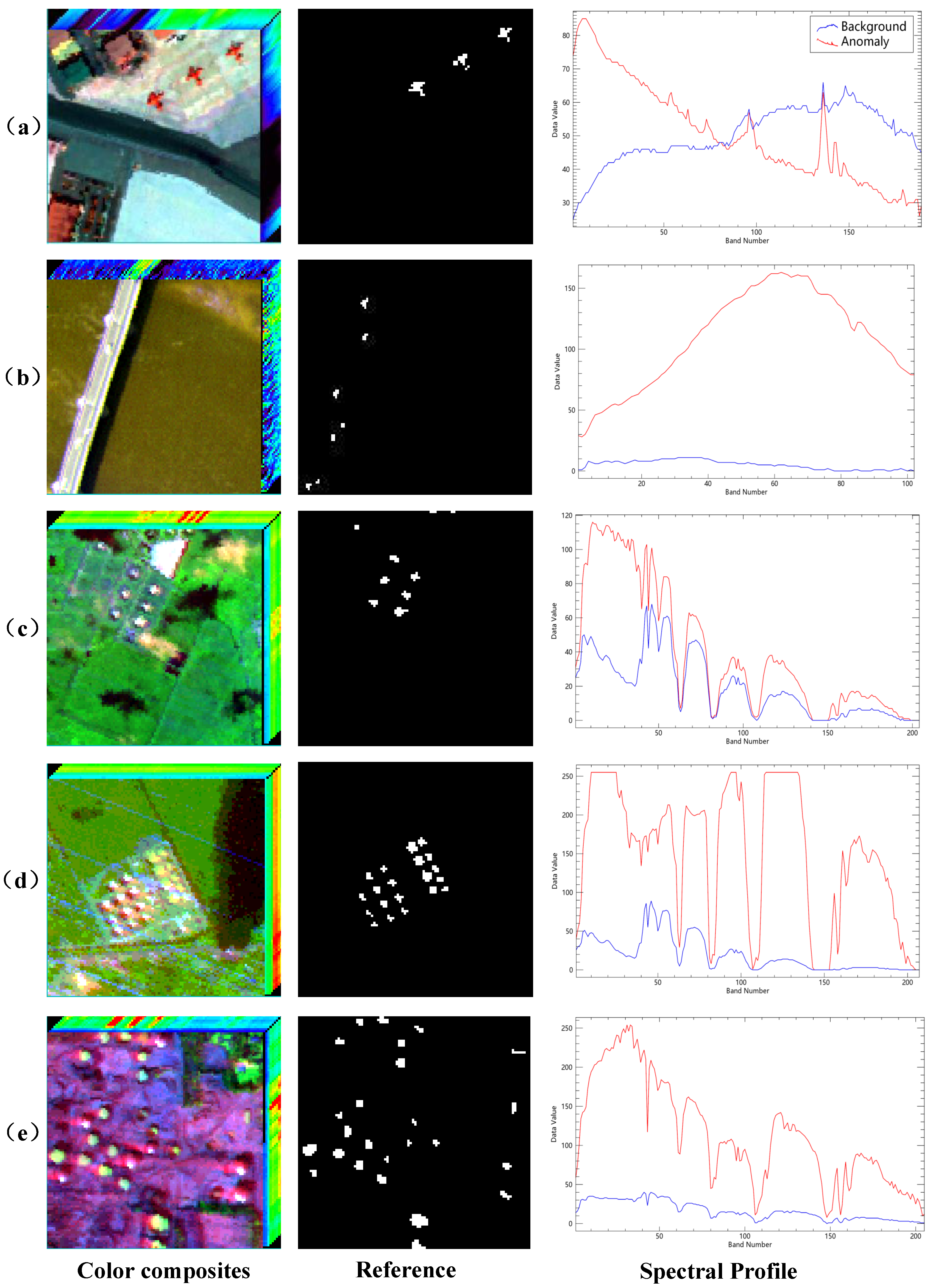
(1) San Diego: The dataset [19] was obtained over the San Diego, California, airport area by the Airborne Visible/Infrared Imaging Spectrometer (AVIRIS). The spectral resolution is 10 nm, while the spatial resolution is around 3.5 m. Its 189 spectral channels have wavelengths between 370 and 2510 nm. The entire photographic scene has a 400 × 400 pixel size. From the top left of the picture, a rectangle of 100 by 100 pixels is chosen and labeled as San Diego. The anomalies in this scene are three aircraft represented by 57 pixels. Figure 2a displays the color composites, reference, and spectral profile of anomalies and background, respectively.

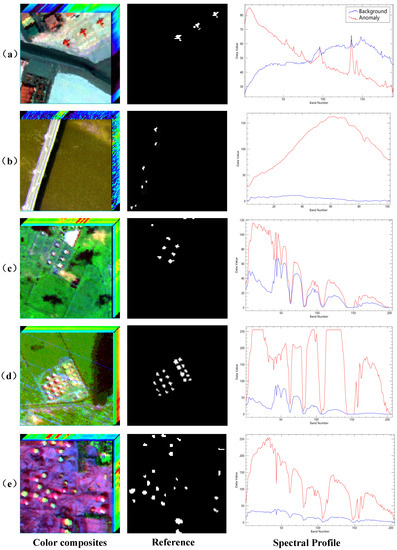
Figure 2. The color composites, reference, and spectral profile for five real hyperspectral datasets: (a) San Diego, (b) Pavia Center, (c) Texas Coast-1, (d) Texas Coast-2, (e) Los Angeles. The red line denotes the spectral curve of anomaly and the blue line denotes the spectral curve of background.

(2) Pavia Center: The dataset was gathered by the Reflective Optics System Imaging Spectrometer (ROSIS) above Pavia Center, Italy, and provides a modest scene with a smooth background. The picture has a resolution of $1.3$ m, a size of $105\times 120$ pixels, and 102 spectral bands. The anomalies are automobiles on the bridge in this scene and the background contains a bridge, bare dirt, and a river. Figure 2b displays the color composites, reference, and spectral profile of anomalies and background, respectively.

(3) Texas Coast-1: This dataset was derived from the AVIRIS sensor over the Texas Coast, TX, USA area. This dataset contains a 100 × 100 pixel picture with 204 spectral bands. Anomalies in this photographic scenario include a variety of man-made targets. The comprehensive acquisition has been explained in [65]. Figure 2c displays the color composites, reference, and spectral profile of anomalies and background, respectively.

(4) Texas Coast-2: Similarly, this dataset was also collected from the AVIRIS sensor over a city in Texas Coast, TX, USA. A total of 100 × 100 pixels make up this metropolitan landscape, which has 207 spectral bands with wavelengths spanning from 450 to 1350 nm. The resolution is 17.2 m/pixel in space. Three motorways and a section of grassland comprise most of the setting. In this scenario, houses are thought to be abnormalities. The substantial strip noise that has distorted this HSI made it difficult to find the above anomalous pixels. Figure 2d displays the color composites, reference, and spectral profile of anomalies and background, respectively.

(5) Los Angeles: This dataset originated from the 7.1 m spatially resolved AVIRIS sensor. After bands selection, this photographic scene, which has a 100 × 100 pixels area, contains 205 spectral bands with wavelengths ranging from 400 to 2500 nm, and 272 pixels representing oil tanks are classified as anomalies. Figure 2e displays the color composites, reference, and spectral profile of anomalies and background, respectively.

Table 1 summarizes the details of all datasets. The anomalies in the scenes of Pavia Center, Texas Coast-1, and Texas Coast-2 are small, while the anomalies in the scenes of San Diego and Los Angeles are relatively large and exhibit distinct geometric structures. In addition, except for Pavia Center, which has the least band of 102, the other datasets all have about 200 bands.

Table 1. Details of the five real datasets in the experiment.

Dataset	Sensor	Resolution	Spatial Size	Bands	Type	Proportion	Average Size
San Diego	AVIRIS	3.5 m	$100\times 100$	189	aircraft	0.57%	19
Pavia Center	ROSIS	1.3 m	$105\times 120$	102	automobiles	0.13%	3
Texas Coast-1	AVIRIS	17.2 m	$100\times 100$	204	buildings	0.67%	8
Texas Coast-2	AVIRIS	17.2 m	$100\times 100$	207	buildings	1.55%	9
Los Angeles	AVIRIS	7.1 m	$100\times 100$	205	oil tanks	2.72%	11

3.2. Performance Evaluation Metrics

In the field of anomaly detection in hyperspectral images, the receiver operating characteristic (ROC) [66] and the area under the curve of ROC (AUC) [67] are widely used as quantitative and qualitative criteria to evaluate the precision and effectiveness of the proposed method. The ROC curve is a graphical tool used to assess the performance of binary classifiers. It plots the True Positive Rate against the False Positive Rate at various decision threshold levels. The TPR and FPR are formulated by

$$\mathrm{TPR}=\mathrm{TP}/(\mathrm{TP}+\mathrm{FN}),\mathrm{FPR}=\mathrm{FP}/(\mathrm{FP}+\mathrm{TN})$$

(17)

where $\mathrm{TP}$ (True Positives) denote the number of correctly identified anomalies, $\mathrm{FP}$ (False Positives) denote the number of background pixels falsely identified as anomalies, $\mathrm{TN}$ (True Negatives) denote the number of correctly identified background pixels and $\mathrm{FN}$ (False Negatives) denote the number of actual anomalies falsely identified as background pixels.

As for the AUC, it is a scalar metric that quantifies the overall performance of a binary classifier, taking into account the complete ROC curve. The AUC value ranges from 0 to 1, where a value of 0.5 represents a random classifier, and a value of 1 indicates perfect classification. A higher AUC value suggests that the classifier can better distinguish between positive and negative samples across different thresholds, making it a valuable measure for comparing different hyperspectral anomaly detection algorithms. The AUC is presented as

$$\begin{array}{c}\mathrm{AUC}={\int }_{-\infty }^{+\infty }\mathrm{TPR}\left(Th\right){\mathrm{FPR}}^{\prime }\left(Th\right)d\left(Th\right)\end{array}$$

(18)

where Th denotes various decision threshold levels. Moreover, box and whisker plots (box plots) are also drawn to display the background distribution and potential anomalies. The boxes within the plot represent the range of detection values for both anomalies and the background. The gaps between the background and anomaly boxes demonstrate the separability of the methods and the lengths of background boxes reflect the background suppression of approaches. A higher AUC value, shorter background boxes, and a more significant separation between the anomaly and background boxes generally suggest a better performance of the detector. Besides qualitative comparison, a visual comparison is also utilized to evaluate the performance of different detectors. The higher the brightness, the greater the probability that the pixel is an anomalous object.

3.3. Ablation Study

3.3.1. Parameter Sensitivity Analysis

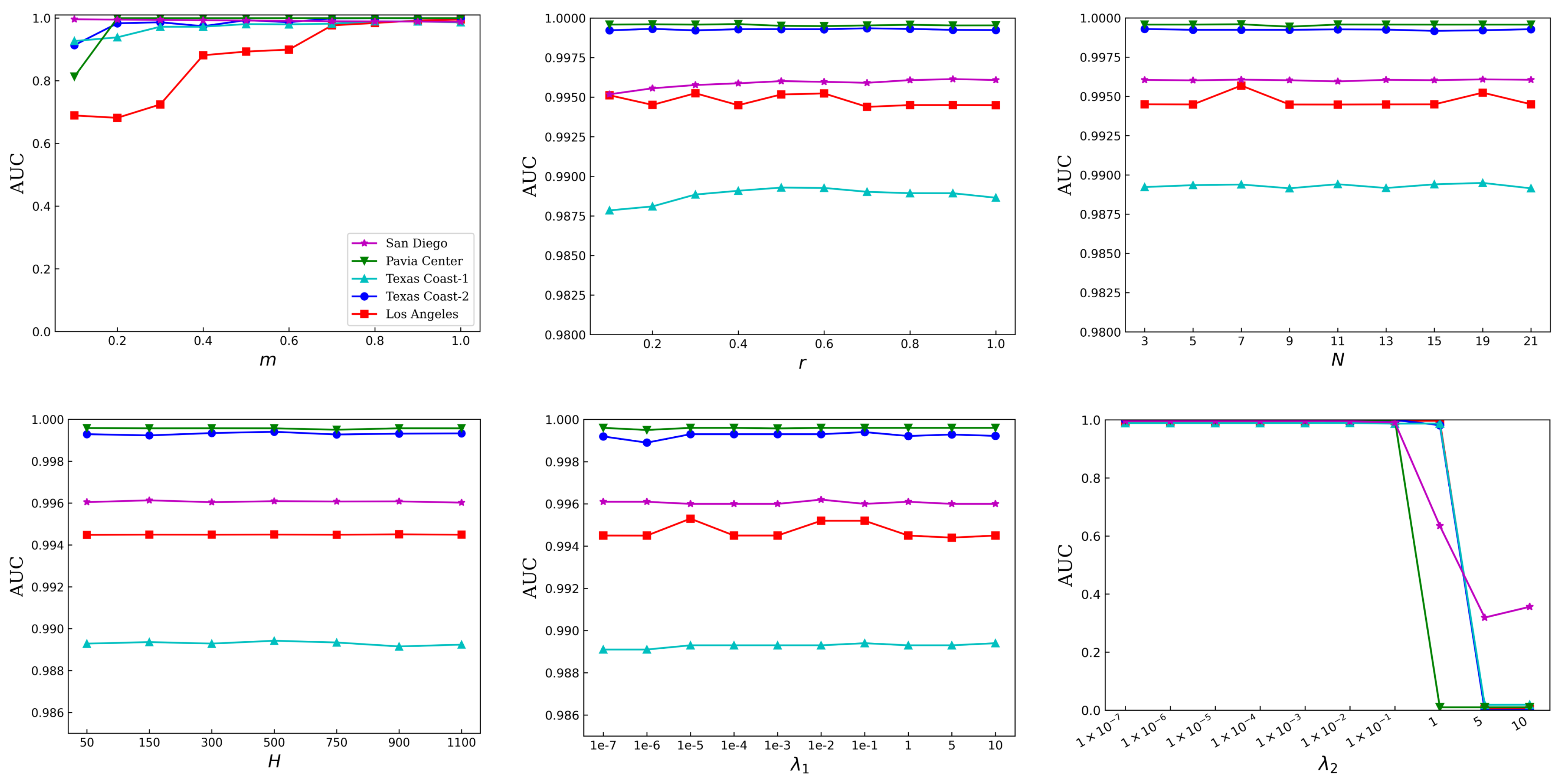
This section analyzes in detail how parameters in different modules affect the effectiveness of the proposed MPGAE approach. Six parameters in the proposed MPGAE detector need to be tuned. The m is the percentage of bands preserved in the module of band selection based on piecewise-smooth prior, r is the coefficient that can decide the dimensionality of the hidden layer, N is the window size of local salient weight, H is the number of superpixels, ${\lambda }_1$ and ${\lambda }_2$ are the tradeoff parameters for the loss terms. In the sensitivity experiment, the other parameters are set to the corresponding fixed value while the study concerning one parameter is conducted. As shown in the subfigures of Figure 3, all datasets are employed. The horizontal axis represents different parameters and the AUC values of (TPR, FPR) are used as the vertical axis. In order to acquire detection results using the optimal parameter combination, the proposed method is adopted with different parameter arrangements to San Diego, Pavia Center, Texas Coast-1, Texas Coast-2, and Los Angeles in turn. Note that in situations of the same accuracy, it tends to select the parameters that minimize the computational time required by the proposed method.

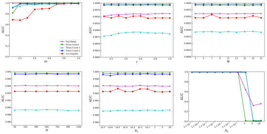
Figure 3. Impact of the parameters on the final detection of the five datasets.

(1) Percentage of bands preserved m: As shown in Figure 3, the value for all datasets ranges from 0.1 to 1 with 0.1 intervals. During training, r is 0.5, N is 11, H is 300, ${\lambda }_1$ and ${\lambda }_2$ are both $1e-3$ for all datesets. For a smaller value of m, the proposed method can capture enough spectral information to detect anomalous targets while the redundant spectral bands can be removed to improve detection performance and computing efficiency. In addition to discarding unnecessary spectral bands, the proposed channel selection can enhance the discriminant of spectral signals by rearranging channels. In Figure 3, it can find that, the performance is more stable to m when m is greater than $0.8$ on most datasets, except the San Diego and Los Angeles. Based on the performance of the proposed MPGAE, the optimal values of m are selected to be {$0.1,0.8,0.8,0.8,1$} for San Diego, Pavia Center, Texas Coast-1, Texas Coast-2, and Los Angeles, respectively.

(2) Coefficient for the dimensionality of hidden layer r: As shown in Figure 3, to reduce the dimension, the ratio for all datasets varies from 0.1 to 1 with 0.1 intervals. During training, m is set as summarized above, N is 11, H is 300, ${\lambda }_1$ and ${\lambda }_2$ are both $1\times {10}^{-3}$ for all datasets. For a small value of r, the AE is incapable of achieving the best representation for the feature, while a large r may lead to overfitting, which results in the decreasing of AUC. Overall, increasing the hidden layer dimension of a neural network can limitedly improve the scores of AUC. In case of the same performance, it is prone to the smaller value, which can avoid overfitting. The optimal values of r are selected to be {$0.8,0.1,0.5,0.7,0.3$} for San Diego, Pavia Center, Texas Coast-1, Texas Coast-2, and Los Angeles, respectively.

(3) Window size of local salient weight N: Although the proposed module incorporates global and local saliency extraction, it employs only a single parameter. This is due to the adaptive calculating of global salient weight adopting a multivariate Gaussian distribution, while the parameter setting of local saliency is solely required for the size of the window. Since the local salient size of window N is an important parameter, the proposed MPGAE may be sensitive to the N. Therefore, by fixing the other parameters as above, and varying N from 3 to 21, the performance of the MPGAE is collected. As shown in Figure 3, the performance of the MPGAE is relatively stable, which reflects the robustness of the proposed MPGAE to some extent. Its robustness proves the certain universality of the assumption that the abnormal pixels are salient in their surroundings. The optimal values of N are selected to be {$3,3,19,7,7$} for San Diego, Pavia Center, Texas Coast-1, Texas Coast-2, and Los Angeles, respectively.

(4) Number of superpixels H: The quality of the local geometric structure is based on the number of segments. For the sensitivity analysis, the H varies from 50 to 1100, the other parameters are fixed as the previous selections. Based on the experimental results in Figure 3, it can be observed that the proposed MPGAE is also insensitive to the number of superpixels H. By weighing precision and running time, the optimal values of H are selected to be {$50,50,500,500,750$} for San Diego, Pavia Center, Texas Coast-1, Texas Coast-2, and Los Angeles, respectively.

(5) Balanced parameters ${\lambda }_1$: The ${\lambda }_1$ adjust the contributions of graph regularization with the Laplacian matrix to the final detection performance. If the ${\lambda }_1$ is too small, the network will not pay enough attention to retain the local geometric features. In contrast, if the ${\lambda }_1$ is too large, the reconstruction of AE and adaptive weight will be ignored. The ${\lambda }_1$ varies from $1\times {10}^{-7}$ to 10. Similarly, the other parameters are selected by the suggestions of the previous analysis. The ablation experiments are shown in Figure 3, like the N and H, and the performance of the proposed method is insensitive to the change of ${\lambda }_1$. The main reason is that the constraint of local geometric structure can provide a robust reconstruction of the background. And the optimal values of N are selected to be $1\times {10}^{-1}$, $1\times {10}^{-3}$, $1\times {10}^{-1}$, $1\times {10}^{-3}$, $1\times {10}^{-2}$ for San Diego, Pavia Center, Texas Coast-1, Texas Coast-2, and Los Angeles, respectively.

(6) Balanced parameters ${\lambda }_2$: The ${\lambda }_1$ adjust the contributions of adaptive salient weight to the final detection performance. If the ${\lambda }_2$ is too small, the network will not pay enough attention to the adaptive weight based on salient prior. Furthermore, if the ${\lambda }_2$ is too large, the reconstruction of AE and the constraint graph regularization will be ignored. The strategy of setting the ${\lambda }_2$ is as same as the sensitivity analysis of ${\lambda }_1$. As shown in Figure 3, with the increase of ${\lambda }_2$, the performance is relatively stable, until ${\lambda }_2$ reaches a certain value, and the performance drops sharply. The main reason is that a large ${\lambda }_2$ compels the network to concentrate on the saliency attributes too much while neglecting the combination of reconstruction error and graph regularization. The optimal values of N are selected to be {$1\times {10}^{-2}$, $1\times {10}^{-1}$, $1\times {10}^{-3}$, $1\times {10}^{-1}$, 1} for San Diego, Pavia Center, Texas Coast-1, Texas Coast-2, and Los Angeles, respectively.

In brief, except for the percentage of bands preserved m, the coefficient for the dimensionality of hidden layer r, and the regularization parameters ${\lambda }_2$, the proposed MPGAE is robust to most parameters. Therefore, it should pay more attention to the setting of the three parameters in applications. Table 2 shows the setting of parameters for different datasets. These experimental results provide valuable insights into the sensitivity of the proposed method to the parameters and can be applied to further optimize the detection performance.

Table 2. The parameters setting for the five real datasets.

Dataset	m	r	N	H	${\mathit{\lambda }}_1$	${\mathit{\lambda }}_2$	AUC
San Diego	0.1	0.8	3	50	$1\times {10}^{-1}$	$1\times {10}^{-2}$	0.9965
Pavia Center	0.8	0.1	3	50	$1\times {10}^{-3}$	$1\times {10}^{-1}$	0.9997
Texas Coast-1	0.8	0.5	19	500	$1\times {10}^{-1}$	$1\times {10}^{-3}$	0.9895
Texas Coast-2	0.8	0.7	7	500	$1\times {10}^{-3}$	$1\times {10}^{-1}$	0.9994
Los Angeles	1	0.3	7	750	$1\times {10}^{-2}$	1	0.9969

3.3.2. Component Analysis

To study the effectiveness of the proposed components, this section discusses the ablation experiments conducted with the autoencoder (AE), Ranking-based band selection with piecewise-smooth prior (RBSPP), adaptive weight based on salient prior (AWBSP), graph regularization (GR) and their combinations. Table 3 shows the AUC scores of ablation experiments on all datasets.

Table 3. AUC scores for ablation study on five datasets.

Dataset	AE	RBSPP	AWBSP	GR	AUC
San Diego	✔				0.9689
	✔	✔			0.9860
	✔	✔	✔		0.9958
	✔	✔	✔	✔	0.9965
Pavia Center	✔				0.9994
	✔	✔			0.9996
	✔	✔	✔		0.9996
	✔	✔	✔	✔	0.9997
Texas Coast-1	✔				0.9876
	✔	✔			0.9889
	✔	✔	✔		0.9892
	✔	✔	✔	✔	0.9895
Texas Coast-2	✔				0.9989
	✔	✔			0.9987
	✔	✔	✔		0.9993
	✔	✔	✔	✔	0.9994
Los Angeles	✔				0.9895
	✔	✔			0.9931
	✔	✔	✔		0.9945
	✔	✔	✔	✔	0.9969

(1) RBSPP Effectiveness: The main function of the RBSPP is to reduce the computational burden and the interference of unnecessary spectral information which can improve the detection performance. As seen from Table 3, compared with the AE without the RBSPP, the combination achieves higher AUC scores on all datasets except the Texas Coast-2. After the RBSPP is added to AE, the AUC scores increased to $0.9860$, $0.9996$, $0.9889$, and $0.9931$ for San Diego, Pavia Center, Texas Coast-1, and Los Angeles, respectively. It can prove that the proposed RBSPP module can remove redundant spectral bands to achieve more accurate detection.

(2) AWBSP Effectiveness: The AWBSP consists of two branches that can calculate the saliency of hyperspectral samples in the local and global contexts, respectively. As shown in Table 3, after adding the AWBSP to the AE with RBSPP, the performance of the combination is better on most datasets except the Pavia Center. The AUC scores increased to $0.9958$, $0.9892$, $0.9994$, and $0.9945$ for San Diego, Texas Coast-1, Texas Coast-2, and Los Angeles, respectively, which shows the advantages of the proposed AWBSP module.

(3) GR Effectiveness: The final ablation experiments are designed to evaluate the effectiveness of the graph regularization. Based on incorporating the GR, the previous combination can preserve the local geometrical attributes in latent feature space. As it can see from Table 3, the AUC scores of the complete version reach $0.9965$, $0.9997$, $0.9895$, $0.9994$, and $0.9969$ for San Diego, Pavia Center, Texas Coast-1, Texas Coast-2, and Los Angeles, respectively. It means the module can improve its performance by preserving the spatial information with local graph constraints.

3.4. Detection Performance Comparison

In this section, to evaluate the competitiveness of the proposed detector, called MPGAE, we chose to compare it with eleven state-of-the-art HAD detectors as follows: RX [26], LRX [27], CRD [37], FRFE [25], IFEBP [68], KIFD [34], SSIIFD [35], RGAE [52], GAED [53], NJCR [38], and KNJCR [38]. The codes of all comparison methods are obtained by well-established open release. The parameters of comparison methods are followed with the setting in their publications. As for the proposed MPGAE, the parameters are set as in the study in Section 3.3.1. The detection results are demonstrated in box and whisker diagrams (Figure 4), ROC curves (Figure 5), AUC scores (Table 4), time consumption (Table 5) and visual comparison (Figure 6, Figure 7, Figure 8, Figure 9 and Figure 10) for five real hyperspectral datasets, respectively.

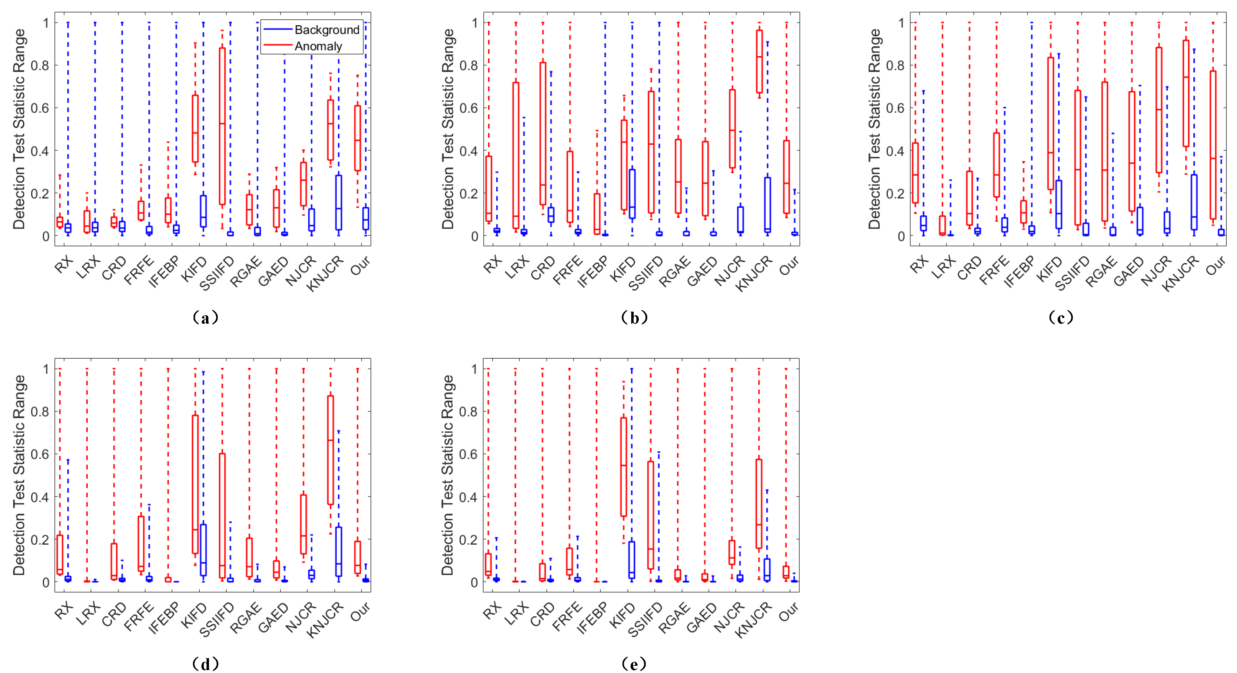
Figure 4. The box and whisker diagrams of the background-anomalies separability of different method comparisons for the five real datasets: (a) San Diego, (b) Pavia Center, (c) Texas Coast-1, (d) Texas Coast-2, (e), and Los Angeles. The red boxes are the detection test statistic range of anomalies, while the blue boxes denote the detection test statistic range of background.

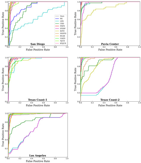
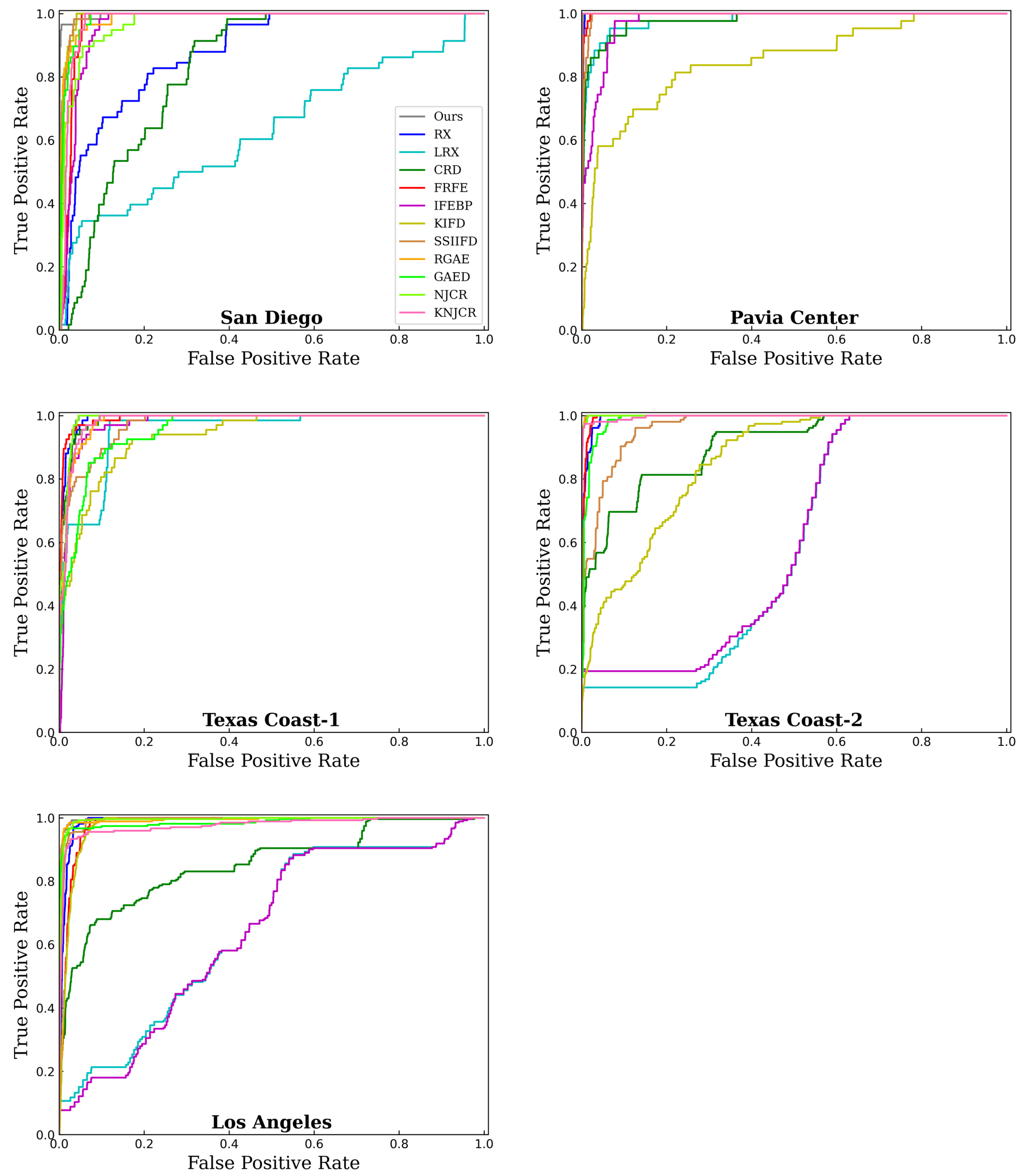
Figure 5. ROC curves for the five datasets.

Table 4. The AUC scores acquired by different HAD methods for the five real datasets.

Methods	San Diego	Pavia Center	Texas Coast-1	Texas Coast-2	Los Angeles	Average
RX	0.8789	0.9982	0.9908	0.9939	0.9893	0.9702
LRX	0.6313	0.9792	0.9512	0.5848	0.6497	0.7592
CRD	0.8282	0.9791	0.9878	0.9048	0.8523	0.9104
FRFE	0.9741	0.9978	0.9916	0.9951	0.9805	0.9878
IFEBP	0.9641	0.9750	0.9764	0.6042	0.6414	0.8322
KIFD	0.9896	0.8507	0.9416	0.8566	0.9786	0.9234
SSIIFD	0.9921	0.9950	0.9719	0.9661	0.9914	0.9833
RGAE	0.9863	0.9997	0.9824	0.9994	0.9945	0.9925
GAED	0.9861	0.9994	0.9533	0.9885	0.9865	0.9828
NJCR	0.9709	0.9996	0.9886	0.9992	0.9944	0.9905
KNJCR	0.9787	0.9996	0.9838	0.9971	0.9772	0.9873
MPGAE	0.9965	0.9997	0.9895	0.9994	0.9969	0.9964

Table 5. The time consuming (seconds) of different HAD methods for the five real datasets.

Methods	San Diego	Pavia Center	Texas Coast-1	Texas Coast-2	Los Angeles	Average
RX	0.09	0.03	0.28	0.16	0.25	0.16
LRX	61.20	48.41	111.83	143.53	155.90	86.84
CRD	9.77	11.75	10.16	11.72	12.66	11.21
FRFE	34.95	49.23	57.08	68.36	75.77	57.08
IFEBP	3.00	2.11	3.53	2.77	2.69	2.82
KIFD	51.62	85.94	74.50	85.31	108.47	81.17
SSIIFD	23.84	20.34	29.11	27.64	33.83	26.95
RGAE	57.36	49.28	47.33	66.14	65.20	43.92
GAED	85.38	107.13	61.84	81.98	85.23	84.31
NJCR	6.5	8.13	4.72	5.39	7.02	6.35
KNJCR	37.17	44.52	30.44	32.97	39.19	36.86
MPGAE	18.28	62.88	123.29	75.44	136.58	83.30

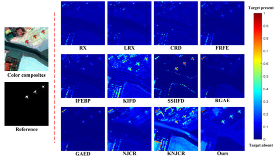
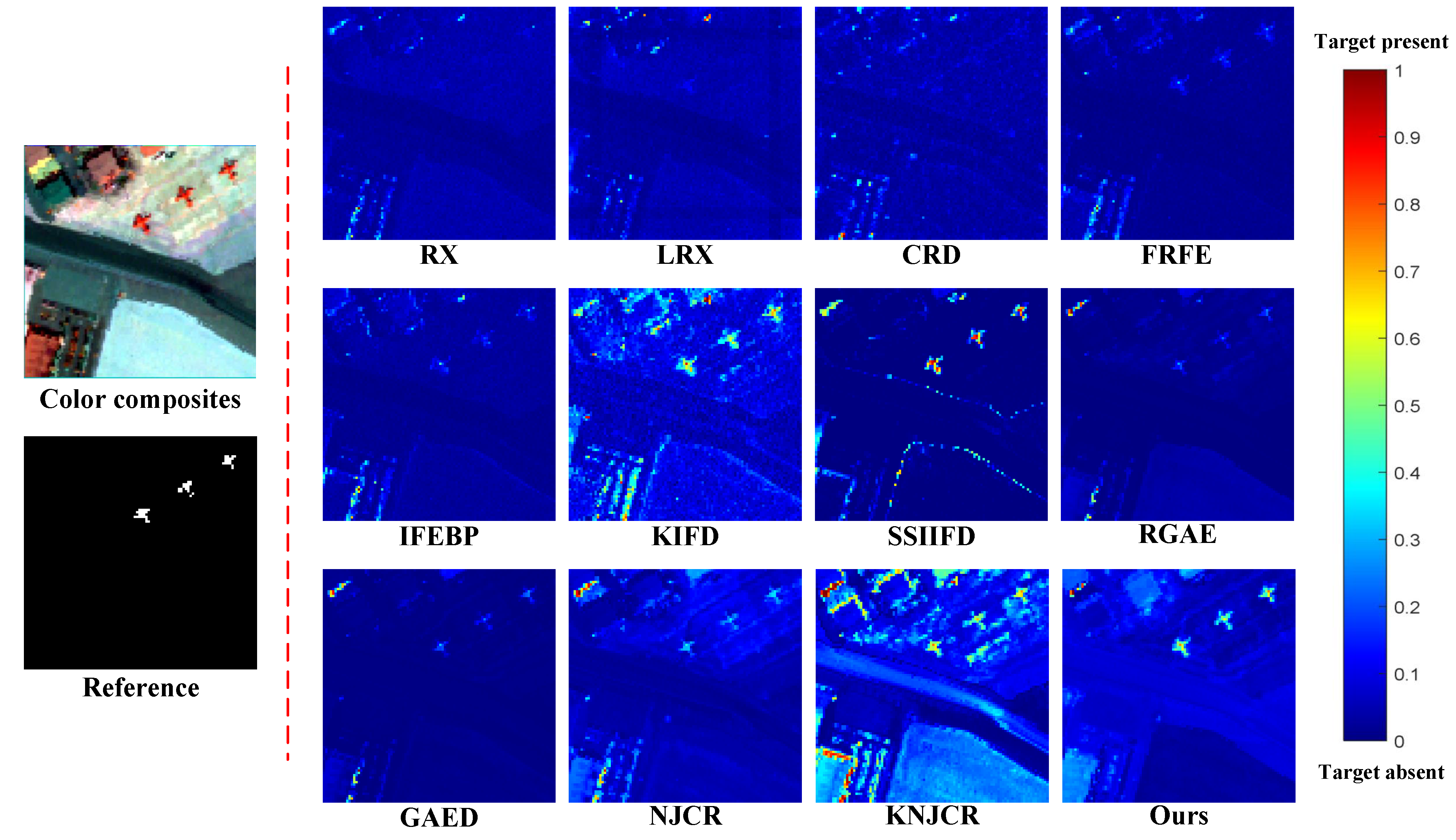
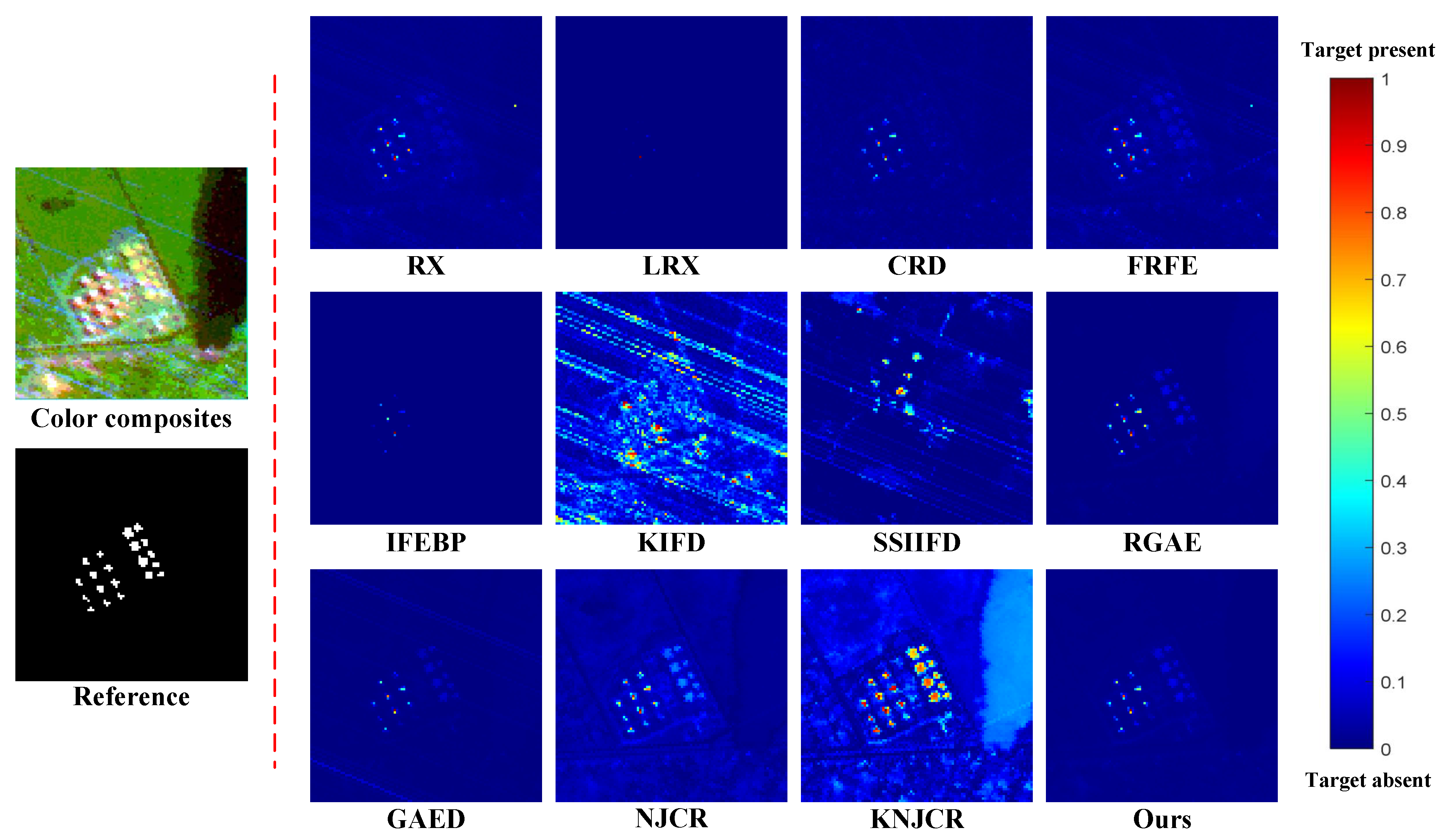
Figure 6. Color detection maps acquired by different HAD methods On the San Diego dataset for visual comparison.

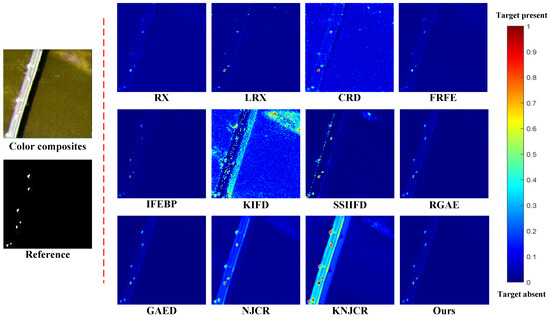
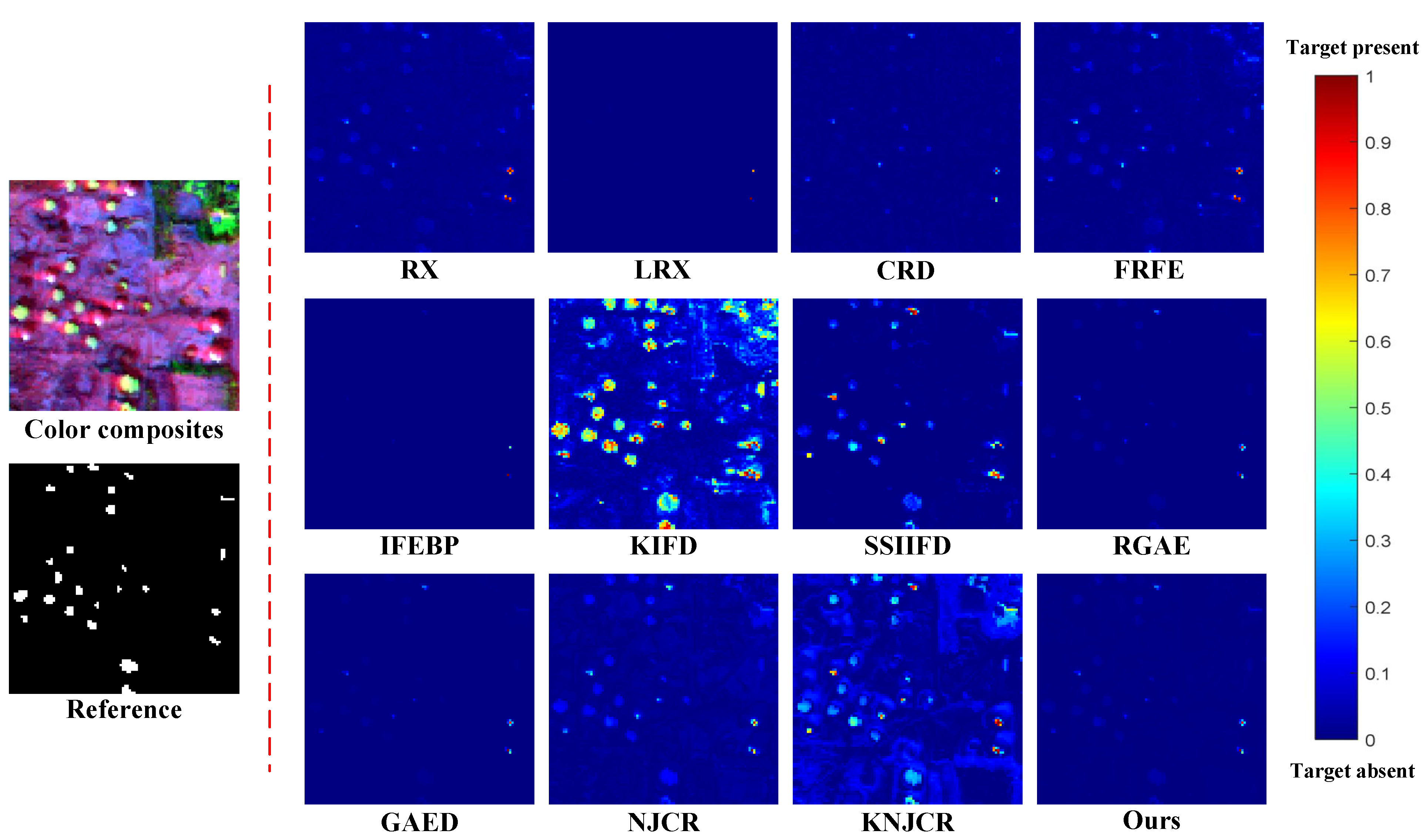
Figure 7. Color detection maps acquired by different HAD methods On the Pavia Center dataset for visual comparison.

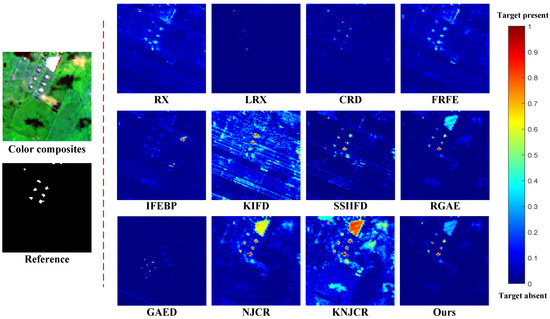
Figure 8. Color detection maps acquired by different HAD methods On the Texas Coast-1 dataset for visual comparison.

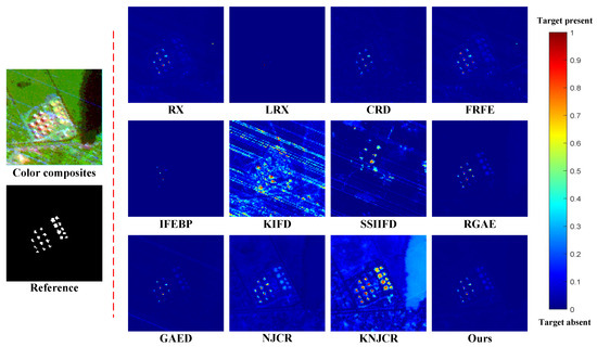
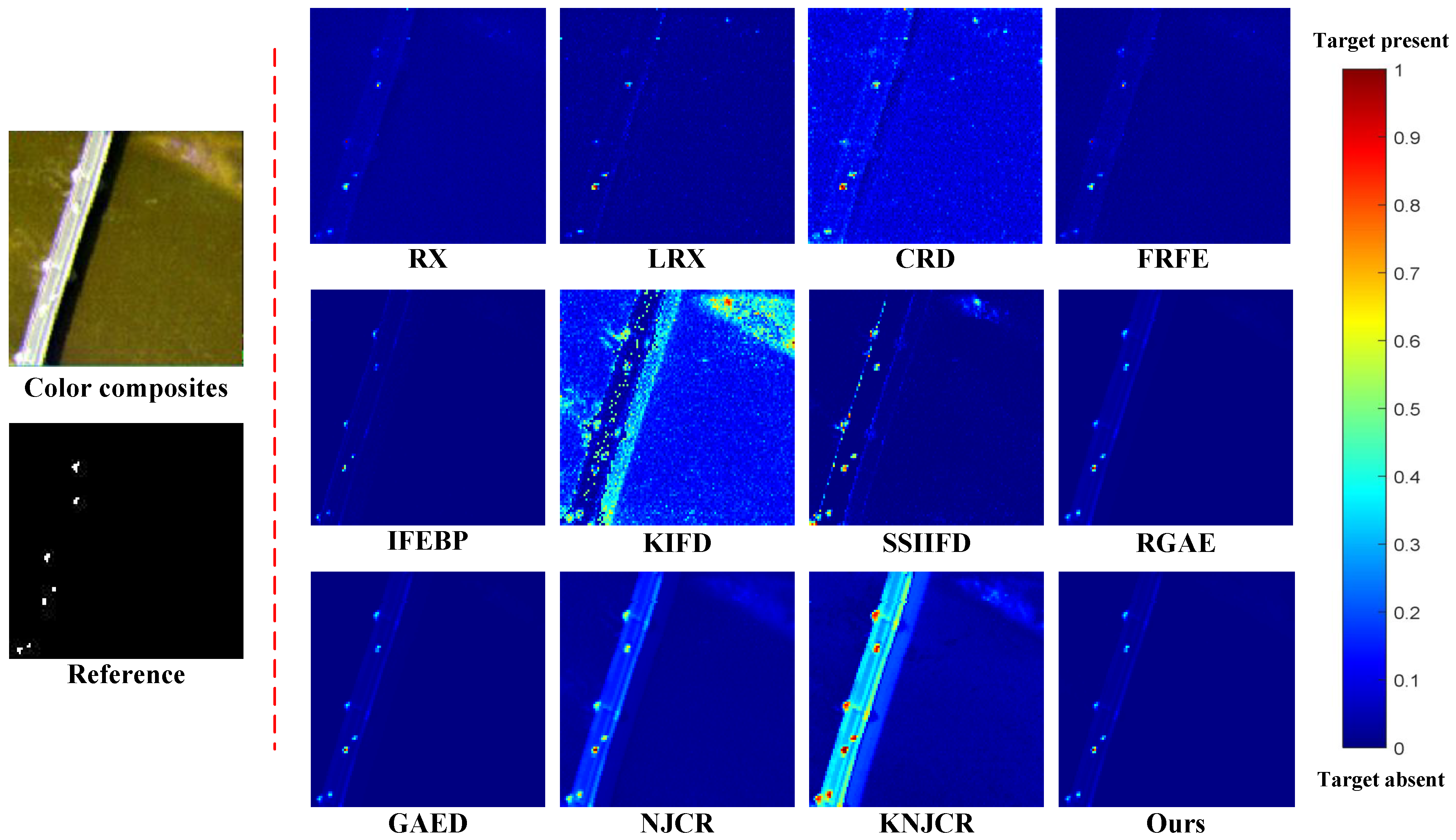
Figure 9. Color detection maps acquired by different HAD methods On the Texas Coast-2 dataset for visual comparison.

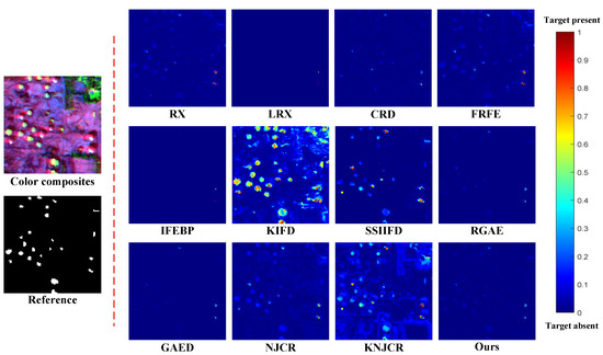
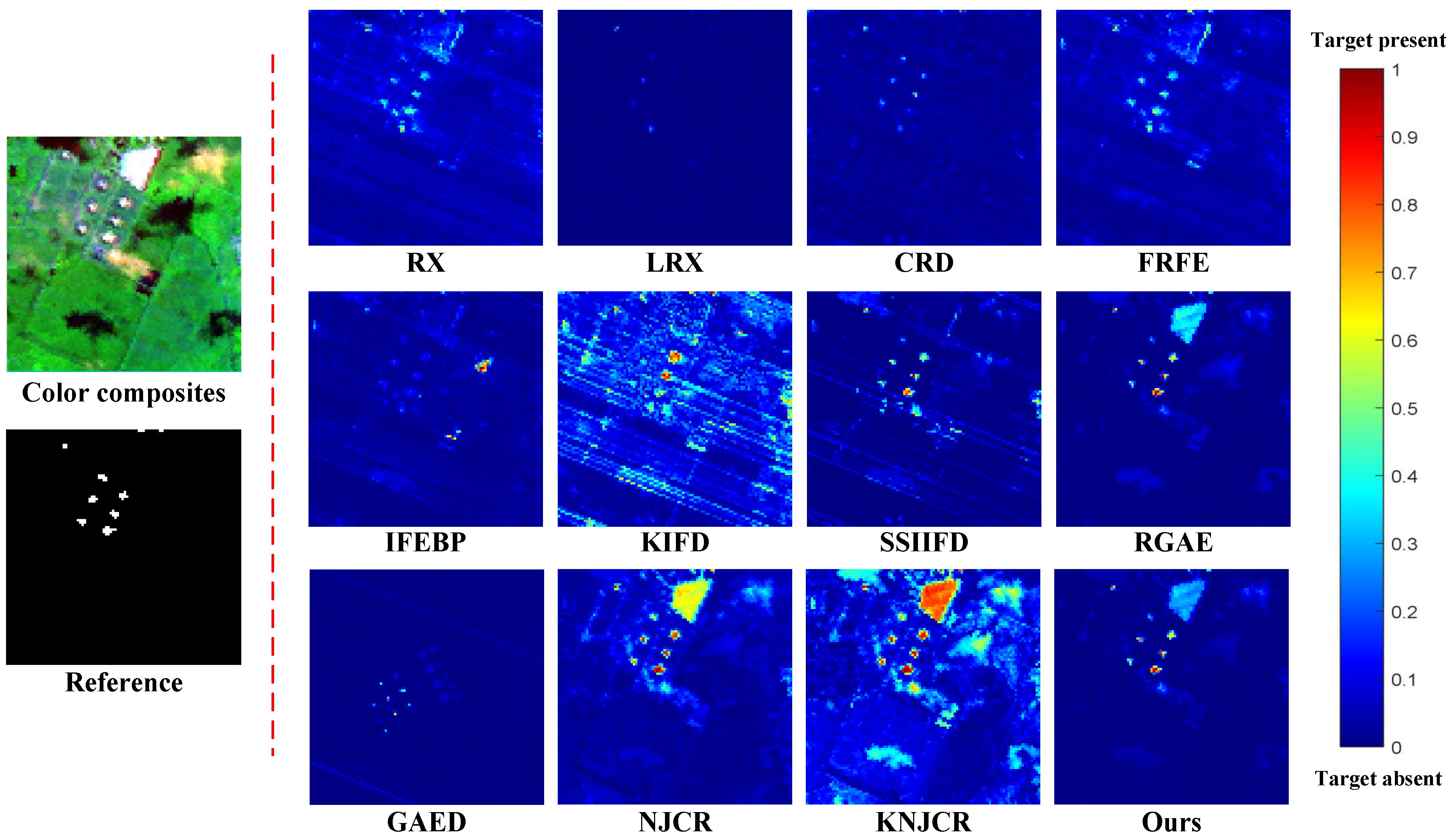
Figure 10. Color detection maps acquired by different HAD methods On the Los Angeles dataset for visual comparison.

3.4.1. San Diego

For the San Diego dataset, as shown in Figure 5 and Table 4, the proposed MPGAE achieves a competitive performance with the highest AUC of $0.9965$. The SSIIFD and KIFD have the second and third highest scores of AUC which are $0.9921$ and $0.9896$, respectively. In addition, Figure 6 draws the color detection maps for various methods on the San Diego dataset. Compared with the other approaches, the proposed MPGAE highlights the targets accurately with clear shapes. Although KIFD, SSIIFD, NJCR, and KNJCR also describe the planes, they are disturbed by noise and misclassifying some of the background pixels. And the other methods fail to display the abnormal regions markedly. Then, the ROC curves also depict that the proposed MPGAE is closer to the top-left corner than the other methods. As for the box and whisker diagrams shown in Figure 4a, the KIFD and the proposed MPGAE have the best separation degree for background and the anomalies while the MPGAE suppresses the background better than KIFD. The GAED obtains the best background suppression; the RX, LRX, and GRX fail to separate the target pixels from the background. Moreover, the computing time of the proposed MPGAE is $18.28s$ which is less than most other methods.

3.4.2. Pavia Center

Figure 5 and Table 4 show the ROC curves and AUC scores generated by different methods, the proposed MPGAE and RGAE obtain the highest AUC of $0.9997$. The NJCR and KNJCR have the second-highest scores of AUC, which are $0.9996$. Except for the KIFD, most methods can achieve high detection performance on the dataset. The main reason is that the background of the Pavia Center dataset is smooth and straightforward. In Figure 7, the KIFD classifies many, background pixels as targets and generates lots of noise. Although the NJCR and KNJCR have satisfactory scores, they emphasize the pixels of the bridge which belong to the background. The SSIIFD, NJCR, KNJCR, and CRD generate the misclassification in the top-right beach which has smoothness as the bridge. The RX and FRFE only highlight partial anomalies. In the box and whisker diagrams Figure 4b, most methods can separate the anomalies and background except KIFD whose boxes of anomalies and background are overlapped. Although KNJCR has the largest gap between the part of anomalies and background, it is unable to suppress the background effectively. In contrast, the IFEBP obtains the best suppression of background, it fails to separate the pixels which belong to different categories. The running time of MPGAE is 62.88 s which has no significant advantage over other methods. Considering the ROC curve, AUC scores, and color detection maps, RGAE and the proposed MPGAE are quite near to one another. As for other metrics, the running time of RGAE is smaller than MPGAE while MPGAE provides better background suppression. The running time of MPGAE is 62.88 s which is less than KIFD and GAED.

3.4.3. Texas Coast-1

As shown in Figure 5 and Table 4, the FRFE has the best score of AUC, which is $0.9916$.The RX and the proposed have the second and third highest scores of AUC which are $0.9921$ and $0.9896$, respectively. All comparison methods can achieve higher scores than $0.90$ for AUC. As for the visual comparison demonstrated in Figure 8, the performance of KIFD and KNJCR is seriously disturbed. The RX, CRD, FRFE, IFEBP, and SSIIFD generate the detection map with substantial strip noise, which means these methods have a limited capacity to suppress noise. Although the MPGAE is robust to the substantial strip noise and locates automobiles and human-made targets clearly, it fails to filter pixels of the other building. At the same time, RGAE suffers from the same issues with more serious distractions whose wrong predictions are brighter. In Figure 4b, in contrast to other methods, the proposed MPGAE is able to suppress the background with a clear separation degree.

3.4.4. Texas Coast-2

The proposed MPGAE and RGAE obtain the highest AUC of $0.9994$ in the Texas Coast-2. The NKCR and KNJCR have the second and third highest scores of AUC which are $0.9992$ and $0.9971$, respectively. The LRX and IFEBP fail to detect the anomalies effectively. As for the color detection maps in Figure 9, NJCR has the best visual performance, and the MPGAE has the second best visual result while the map of KIFD is full of substantial strip noise, the same as SSIIFD. The LRX fails to generate the color maps with meaningful prediction. The box and whisker diagrams of the Texas Coast-2 dataset are described in Figure 4d. Although the RGAE realizes the best background suppression, its boxes of background and anomalies are almost overlapped. In contrast, KNJCR has the best separation degree while its ability is weak for suppressing background. The proposed MPGAE has balanced suppression and separation degrees for the anomalies and their surroundings. The running time of MPGAE is $75.44s$ which is less than LRX, KIFD and GAED.

3.4.5. Los Angeles

Similar to the comparative result of the other datasets, the proposed MPGAE realizes the highest AUC whose score is $0.9969$ in Los Angeles. The RGAE and KNJCR have the second- and third-highest scores of AUC which are $0.9945$ and $0.9944$, respectively. The color detection map of NJCR shows the shapes of oil tanks and partial backgrounds. In Figure 10, The KIFD highlights the oil and partial background at the same time which makes it hard to locate targets. In addition, the detection results of the KIFD contain a lot of noise. Although the probability values of anomalies are low in the color detection map of MPGAE, it is still much higher than the background which makes the abnormal pixels able to be identified. As for the analysis of the separation degree and suppression in Figure 4e, the proposed method can effectively suppress background with a smaller range than SSIIFD. And the CRD cannot diagnose the targets from the boxes.

By employing the eleven state-of-the-art HAD methods, comprehensive comparison experiments are conducted on five real datasets to demonstrate the superiority of the proposed MPGAE which achieves the best performance on four datasets and has the greatest average scores of AUC $0.9964$. The average running time of the proposed method is 85.05s. Moreover, as drawn in the box diagrams, it can be concluded that the proposed MPGAE cannot only suppress the background, but also isolate the anomaly effectively. Although the processing time of RX and IFEBP are fast, their performance is not excellent, especially for their visual detection maps. As for the AE-based methods, such as RGAE, GAED, and the proposed MPGAE, the running time contains the training time and detecting time. The running time of the proposed MPGAE is close to GAED. Based on overall consideration of the detection performance and the time consumption, the proposed MPGAE is more effective for HAD tasks.

4. Conclusions

This paper presents a novel HAD approach called MPGAE that contains band selection, adaptive weight, and graph regularization. The band selection can reduce redundant spectral information, enhance the discriminant ability, and decrease computing consumption. In addition, the adaptive weight can characterize the anomalies by adjusting the reconstruction capacity of the AE by highlighting the spectral difference of samples in local and global contexts. As for the graph regularization, it can retain essential local geometric features by structuring the Laplacian matrix on the superpixels provided by segmentation. According to experimental results on five real scenes, the proposed MPGAE effectively suppresses the background and accurately separates anomalies by modeling a more accurate background distribution. The proposed MPGAE outperforms all other methods on the relatively complex scenes of San Diego and Los Angeles, with respective AUC scores of $0.9965$ and $0.9969$. And it achieves the best average AUC score of $0.9964$ with an $85.05s$ average runtime. In the future, our research will concentrate on how to decrease the complexity of the MPGAE and enable it to achieve one-step detection.

References

- Goetz, A.F.; Vane, G.; Solomon, J.E.; Rock, B.N. Imaging spectrometry for earth remote sensing. Science 1985, 228, 1147–1153. [Google Scholar] [CrossRef]
- Lin, M.; Yang, G.; Zhang, H. Transition is a process: Pair-to-video change detection networks for very high resolution remote sensing images. IEEE Trans. Image Process. 2022, 32, 57–71. [Google Scholar] [CrossRef] [PubMed]
- Tong, X.; Pan, H.; Liu, S.; Li, B.; Luo, X.; Xie, H.; Xu, X. A novel approach for hyperspectral change detection based on uncertain area analysis and improved transfer learning. IEEE J. Sel. Top. Appl. Earth Obs. Remote Sens. 2020, 13, 2056–2069. [Google Scholar] [CrossRef]
- Liu, S.; Song, L.; Li, H.; Chen, J.; Zhang, G.; Hu, B.; Wang, S.; Li, S. Spatial weighted kernel spectral angle constraint method for hyperspectral change detection. J. Appl. Remote Sens. 2022, 16, 016503. [Google Scholar] [CrossRef]
- Liu, S.; Li, H.; Chen, J.; Li, S.; Song, L.; Zhang, G.; Hu, B. Adaptive convolution kernel network for change detection in hyperspectral images. Appl. Opt. 2023, 62, 2039–2047. [Google Scholar] [CrossRef]
- Fang, J.; Cao, X. Multidimensional relation learning for hyperspectral image classification. Neurocomputing 2020, 410, 211–219. [Google Scholar] [CrossRef]
- Shi, Y.; Fu, B.; Wang, N.; Cheng, Y.; Fang, J.; Liu, X.; Zhang, G. Spectral-Spatial Attention Rotation-Invariant Classification Network for Airborne Hyperspectral Images. Drones 2023, 7, 240. [Google Scholar] [CrossRef]
- Zhang, X.; Yang, S.; Feng, Z.; Song, L.; Wei, Y.; Jiao, L. Triple Contrastive Representation Learning for Hyperspectral Image Classification with Noisy Labels. IEEE Trans. Geosci. Remote Sens. 2023. [Google Scholar] [CrossRef]
- Chen, Y.; Huang, J.; Mou, L.; Jin, P.; Xiong, S.; Zhu, X.X. Deep Saliency Smoothing Hashing for Drone Image Retrieval. IEEE Trans. Geosci. Remote Sens. 2023, 61, 4700913. [Google Scholar] [CrossRef]
- Zhang, X.; Fan, X.; Wang, G.; Chen, P.; Tang, X.; Jiao, L. MFGNet: Multibranch Feature Generation Networks for Few-Shot Remote Sensing Scene Classification. IEEE Trans. Geosci. Remote Sens. 2023, 61, 5609613. [Google Scholar] [CrossRef]
- Li, Y.; Chen, R.; Zhang, Y.; Zhang, M.; Chen, L. Multi-label remote sensing image scene classification by combining a convolutional neural network and a graph neural network. Remote Sens. 2020, 12, 4003. [Google Scholar] [CrossRef]
- Wang, N.; Shi, Y.; Yang, F.; Zhang, G.; Li, S.; Liu, X. Collaborative representation with multipurification processing and local salient weight for hyperspectral anomaly detection. J. Appl. Remote Sens. 2022, 16, 036517. [Google Scholar] [CrossRef]
- Yao, Y.; Wang, M.; Fan, G.; Liu, W.; Ma, Y.; Mei, X. Dictionary Learning-Cooperated Matrix Decomposition for Hyperspectral Target Detection. Remote Sens. 2022, 14, 4369. [Google Scholar] [CrossRef]
- Nassif, A.B.; Talib, M.A.; Nasir, Q.; Dakalbab, F.M. Machine learning for anomaly detection: A systematic review. IEEE Access 2021, 9, 78658–78700. [Google Scholar] [CrossRef]
- Xia, X.; Pan, X.; Li, N.; He, X.; Ma, L.; Zhang, X.; Ding, N. GAN-based anomaly detection: A review. Neurocomputing 2022, 493, 497–535. [Google Scholar] [CrossRef]
- Wang, S.; Wang, X.; Zhong, Y.; Zhang, L. Hyperspectral anomaly detection via locally enhanced low-rank prior. IEEE Trans. Geosci. Remote Sens. 2020, 58, 6995–7009. [Google Scholar] [CrossRef]
- Jiang, K.; Xie, W.; Lei, J.; Li, Z.; Li, Y.; Jiang, T.; Du, Q. E2E-LIADE: End-to-end local invariant autoencoding density estimation model for anomaly target detection in hyperspectral image. IEEE Trans. Cybern. 2021, 52, 11385–11396. [Google Scholar] [CrossRef]
- Chang, C.I.; Chiang, S.S. Anomaly detection and classification for hyperspectral imagery. IEEE Trans. Geosci. Remote Sens. 2002, 40, 1314–1325. [Google Scholar] [CrossRef]
- Xu, Y.; Wu, Z.; Li, J.; Plaza, A.; Wei, Z. Anomaly detection in hyperspectral images based on low-rank and sparse representation. IEEE Trans. Geosci. Remote Sens. 2015, 54, 1990–2000. [Google Scholar] [CrossRef]
- Zhang, X.; Ma, X.; Huyan, N.; Gu, J.; Tang, X.; Jiao, L. Spectral-difference low-rank representation learning for hyperspectral anomaly detection. IEEE Trans. Geosci. Remote Sens. 2021, 59, 10364–10377. [Google Scholar] [CrossRef]
- Wu, Z.; Su, H.; Tao, X.; Han, L.; Paoletti, M.E.; Haut, J.M.; Plaza, J.; Plaza, A. Hyperspectral anomaly detection with relaxed collaborative representation. IEEE Trans. Geosci. Remote Sens. 2022, 60, 5533417. [Google Scholar] [CrossRef]
- Matteoli, S.; Diani, M.; Corsini, G. A tutorial overview of anomaly detection in hyperspectral images. IEEE Aerosp. Electron. Syst. Mag. 2010, 25, 5–28. [Google Scholar] [CrossRef]
- Du, B.; Zhang, L. A discriminative metric learning based anomaly detection method. IEEE Trans. Geosci. Remote Sens. 2014, 52, 6844–6857. [Google Scholar]
- Huyan, N.; Zhang, X.; Zhou, H.; Jiao, L. Hyperspectral anomaly detection via background and potential anomaly dictionaries construction. IEEE Trans. Geosci. Remote Sens. 2018, 57, 2263–2276. [Google Scholar] [CrossRef]
- Tao, R.; Zhao, X.; Li, W.; Li, H.C.; Du, Q. Hyperspectral anomaly detection by fractional Fourier entropy. IEEE J. Sel. Top. Appl. Earth Obs. Remote Sens. 2019, 12, 4920–4929. [Google Scholar] [CrossRef]
- Reed, I.S.; Yu, X. Adaptive multiple-band CFAR detection of an optical pattern with unknown spectral distribution. IEEE Trans. Acoust. Speech Signal Process. 1990, 38, 1760–1770. [Google Scholar] [CrossRef]
- Molero, J.M.; Garzon, E.M.; Garcia, I.; Plaza, A. Analysis and optimizations of global and local versions of the RX algorithm for anomaly detection in hyperspectral data. IEEE J. Sel. Top. Appl. Earth Obs. Remote Sens. 2013, 6, 801–814. [Google Scholar] [CrossRef]
- Zhao, C.; Wang, Y.; Qi, B.; Wang, J. Global and local real-time anomaly detectors for hyperspectral remote sensing imagery. Remote Sens. 2015, 7, 3966–3985. [Google Scholar] [CrossRef]
- Kwon, H.; Nasrabadi, N.M. Kernel RX-algorithm: A nonlinear anomaly detector for hyperspectral imagery. IEEE Trans. Geosci. Remote Sens. 2005, 43, 388–397. [Google Scholar] [CrossRef]
- Gu, Y.; Liu, Y.; Zhang, Y. A selective KPCA algorithm based on high-order statistics for anomaly detection in hyperspectral imagery. IEEE Geosci. Remote Sens. Lett. 2008, 5, 43–47. [Google Scholar] [CrossRef]
- Zhou, J.; Kwan, C.; Ayhan, B.; Eismann, M.T. A novel cluster kernel RX algorithm for anomaly and change detection using hyperspectral images. IEEE Trans. Geosci. Remote Sens. 2016, 54, 6497–6504. [Google Scholar] [CrossRef]
- He, F.; Yan, S.; Ding, Y.; Sun, Z.; Zhao, J.; Hu, H.; Zhu, Y. Recursive RX with Extended Multi-Attribute Profiles for Hyperspectral Anomaly Detection. Remote Sens. 2023, 15, 589. [Google Scholar] [CrossRef]
- Carlotto, M.J. A cluster-based approach for detecting human-made objects and changes in imagery. IEEE Trans. Geosci. Remote Sens. 2005, 43, 374–387. [Google Scholar] [CrossRef]
- Li, S.; Zhang, K.; Duan, P.; Kang, X. Hyperspectral anomaly detection with kernel isolation forest. IEEE Trans. Geosci. Remote Sens. 2019, 58, 319–329. [Google Scholar] [CrossRef]
- Song, X.; Aryal, S.; Ting, K.M.; Liu, Z.; He, B. Spectral–spatial anomaly detection of hyperspectral data based on improved isolation forest. IEEE Trans. Geosci. Remote Sens. 2021, 60, 1–16. [Google Scholar] [CrossRef]
- Zhang, L.; Yang, M.; Feng, X. Sparse representation or collaborative representation: Which helps face recognition? In Proceedings of the 2011 International Conference on Computer Vision, Barcelona, Spain, 6–13 November 2011; IEEE: Piscataway, NJ, USA, 2011; pp. 471–478. [Google Scholar]
- Li, W.; Du, Q. Collaborative representation for hyperspectral anomaly detection. IEEE Trans. Geosci. Remote Sens. 2014, 53, 1463–1474. [Google Scholar] [CrossRef]
- Chang, S.; Ghamisi, P. Nonnegative-Constrained Joint Collaborative Representation With Union Dictionary for Hyperspectral Anomaly Detection. IEEE Trans. Geosci. Remote Sens. 2022, 60, 1–13. [Google Scholar] [CrossRef]
- Li, J.; Zhang, H.; Zhang, L.; Ma, L. Hyperspectral anomaly detection by the use of background joint sparse representation. IEEE J. Sel. Top. Appl. Earth Obs. Remote Sens. 2015, 8, 2523–2533. [Google Scholar] [CrossRef]
- Zhao, R.; Du, B.; Zhang, L.; Zhang, L. A robust background regression based score estimation algorithm for hyperspectral anomaly detection. ISPRS J. Photogramm. Remote Sens. 2016, 122, 126–144. [Google Scholar] [CrossRef]
- Liu, G.; Lin, Z.; Yan, S.; Sun, J.; Yu, Y.; Ma, Y. Robust recovery of subspace structures by low-rank representation. IEEE Trans. Pattern Anal. Mach. Intell. 2012, 35, 171–184. [Google Scholar] [CrossRef]
- Sun, S.; Liu, J.; Zhang, Z.; Li, W. Hyperspectral Anomaly Detection Based on Adaptive Low-Rank Transformed Tensor. IEEE Trans. Neural Netw. Learn. Syst. 2023. early access. [Google Scholar] [CrossRef] [PubMed]
- Qu, Y.; Wang, W.; Guo, R.; Ayhan, B.; Kwan, C.; Vance, S.; Qi, H. Hyperspectral anomaly detection through spectral unmixing and dictionary-based low-rank decomposition. IEEE Trans. Geosci. Remote Sens. 2018, 56, 4391–4405. [Google Scholar] [CrossRef]
- Qu, Y.; Guo, R.; Wang, W.; Qi, H.; Ayhan, B.; Kwan, C.; Vance, S. Anomaly detection in hyperspectral images through spectral unmixing and low rank decomposition. In Proceedings of the 2016 IEEE International Geoscience and Remote Sensing Symposium (IGARSS), Beijing, China, 10–15 July 2016; IEEE: Piscataway, NJ, USA, 2016; pp. 1855–1858. [Google Scholar]
- Song, D.; Dong, Y.; Li, X. Hierarchical edge refinement network for saliency detection. IEEE Trans. Image Process. 2021, 30, 7567–7577. [Google Scholar] [CrossRef] [PubMed]
- Song, D.; Dong, Y.; Li, X. Context and Difference Enhancement Network for Change Detection. IEEE J. Sel. Top. Appl. Earth Obs. Remote Sens. 2022, 15, 9457–9467. [Google Scholar] [CrossRef]
- Li, W.; Wu, G.; Du, Q. Transferred deep learning for anomaly detection in hyperspectral imagery. IEEE Geosci. Remote. Sens. Lett. 2017, 14, 597–601. [Google Scholar] [CrossRef]
- Creswell, A.; Bharath, A.A. Denoising adversarial autoencoders. IEEE Trans. Neural Netw. Learn. Syst. 2018, 30, 968–984. [Google Scholar] [CrossRef]
- Zhao, C.; Zhang, L. Spectral-spatial stacked autoencoders based on low-rank and sparse matrix decomposition for hyperspectral anomaly detection. Infrared Phys. Technol. 2018, 92, 166–176. [Google Scholar] [CrossRef]
- Xie, W.; Lei, J.; Liu, B.; Li, Y.; Jia, X. Spectral constraint adversarial autoencoders approach to feature representation in hyperspectral anomaly detection. Neural Netw. 2019, 119, 222–234. [Google Scholar] [CrossRef]
- Wang, S.; Wang, X.; Zhang, L.; Zhong, Y. Auto-AD: Autonomous hyperspectral anomaly detection network based on fully convolutional autoencoder. IEEE Trans. Geosci. Remote Sens. 2021, 60, 5503314. [Google Scholar] [CrossRef]
- Fan, G.; Ma, Y.; Mei, X.; Fan, F.; Huang, J.; Ma, J. Hyperspectral anomaly detection with robust graph autoencoders. IEEE Trans. Geosci. Remote. Sens. 2021, 60, 5511314. [Google Scholar]
- Xiang, P.; Ali, S.; Jung, S.K.; Zhou, H. Hyperspectral anomaly detection with guided autoencoder. IEEE Trans. Geosci. Remote Sens. 2022, 60, 5538818. [Google Scholar] [CrossRef]
- He, K.; Sun, W.; Yang, G.; Meng, X.; Ren, K.; Peng, J.; Du, Q. A dual global–local attention network for hyperspectral band selection. IEEE Trans. Geosci. Remote Sens. 2022, 60, 5527613. [Google Scholar] [CrossRef]
- Wang, Q.; Li, Q.; Li, X. Hyperspectral band selection via adaptive subspace partition strategy. IEEE J. Sel. Top. Appl. Earth Obs. Remote Sens. 2019, 12, 4940–4950. [Google Scholar] [CrossRef]
- Xie, W.; Lei, J.; Yang, J.; Li, Y.; Du, Q.; Li, Z. Deep latent spectral representation learning-based hyperspectral band selection for target detection. IEEE Trans. Geosci. Remote Sens. 2019, 58, 2015–2026. [Google Scholar] [CrossRef]
- Jiao, C.; Chen, C.; McGarvey, R.G.; Bohlman, S.; Jiao, L.; Zare, A. Multiple instance hybrid estimator for hyperspectral target characterization and sub-pixel target detection. ISPRS J. Photogramm. Remote Sens. 2018, 146, 235–250. [Google Scholar] [CrossRef]
- Ye, F.; Huang, C.; Cao, J.; Li, M.; Zhang, Y.; Lu, C. Attribute restoration framework for anomaly detection. IEEE Trans. Multimed. 2020, 24, 116–127. [Google Scholar] [CrossRef]
- Li, L.; Li, W.; Qu, Y.; Zhao, C.; Tao, R.; Du, Q. Prior-based tensor approximation for anomaly detection in hyperspectral imagery. IEEE Trans. Neural Netw. Learn. Syst. 2020, 33, 1037–1050. [Google Scholar] [CrossRef]
- Achanta, R.; Shaji, A.; Smith, K.; Lucchi, A.; Fua, P.; Süsstrunk, S. SLIC superpixels compared to state-of-the-art superpixel methods. IEEE Trans. Pattern Anal. Mach. Intell. 2012, 34, 2274–2282. [Google Scholar] [CrossRef]
- Su, H.; Wu, Z.; Zhang, H.; Du, Q. Hyperspectral anomaly detection: A survey. IEEE Geosci. Remote Sens. Mag. 2021, 10, 64–90. [Google Scholar] [CrossRef]
- Li, J.; Zhang, H.; Zhang, L. Efficient superpixel-level multitask joint sparse representation for hyperspectral image classification. IEEE Trans. Geosci. Remote Sens. 2015, 53, 5338–5351. [Google Scholar]
- Li, Z.; Liu, J.; Tang, J.; Lu, H. Robust structured subspace learning for data representation. IEEE Trans. Pattern Anal. Mach. Intell. 2015, 37, 2085–2098. [Google Scholar] [CrossRef] [PubMed]
- Ding, C.; Zhou, D.; He, X.; Zha, H. R 1-pca: Rotational invariant l 1-norm principal component analysis for robust subspace factorization. In Proceedings of the 23rd International Conference on Machine Learning, Pittsburgh, PA, USA, 25–29 June 2006; pp. 281–288. [Google Scholar]
- Kang, X.; Zhang, X.; Li, S.; Li, K.; Li, J.; Benediktsson, J.A. Hyperspectral anomaly detection with attribute and edge-preserving filters. IEEE Trans. Geosci. Remote Sens. 2017, 55, 5600–5611. [Google Scholar] [CrossRef]
- Zweig, M.H.; Campbell, G. Receiver-operating characteristic (ROC) plots: A fundamental evaluation tool in clinical medicine. Clin. Chem. 1993, 39, 561–577. [Google Scholar] [CrossRef] [PubMed]
- Ferri, C.; Hernández-Orallo, J.; Flach, P.A. A coherent interpretation of AUC as a measure of aggregated classification performance. In Proceedings of the 28th International Conference on Machine Learning (ICML-11), Bellevue, WA, USA, 28 June–2 July 2011; pp. 657–664. [Google Scholar]
- Ma, Y.; Fan, G.; Jin, Q.; Huang, J.; Mei, X.; Ma, J. Hyperspectral anomaly detection via integration of feature extraction and background purification. IEEE Geosci. Remote Sens. Lett. 2020, 18, 1436–1440. [Google Scholar] [CrossRef]
Disclaimer/Publisher’s Note: The statements, opinions and data contained in all publications are solely those of the individual author(s) and contributor(s) and not of MDPI and/or the editor(s). MDPI and/or the editor(s) disclaim responsibility for any injury to people or property resulting from any ideas, methods, instructions or products referred to in the content. |
© 2023 by the authors. Licensee MDPI, Basel, Switzerland. This article is an open access article distributed under the terms and conditions of the Creative Commons Attribution (CC BY) license (https://creativecommons.org/licenses/by/4.0/).