


Evaluation of Susceptibility by Mass Movements through Stochastic and Statistical Methods for a Region of Bucaramanga, Colombia


Abstract
:
1. Introduction
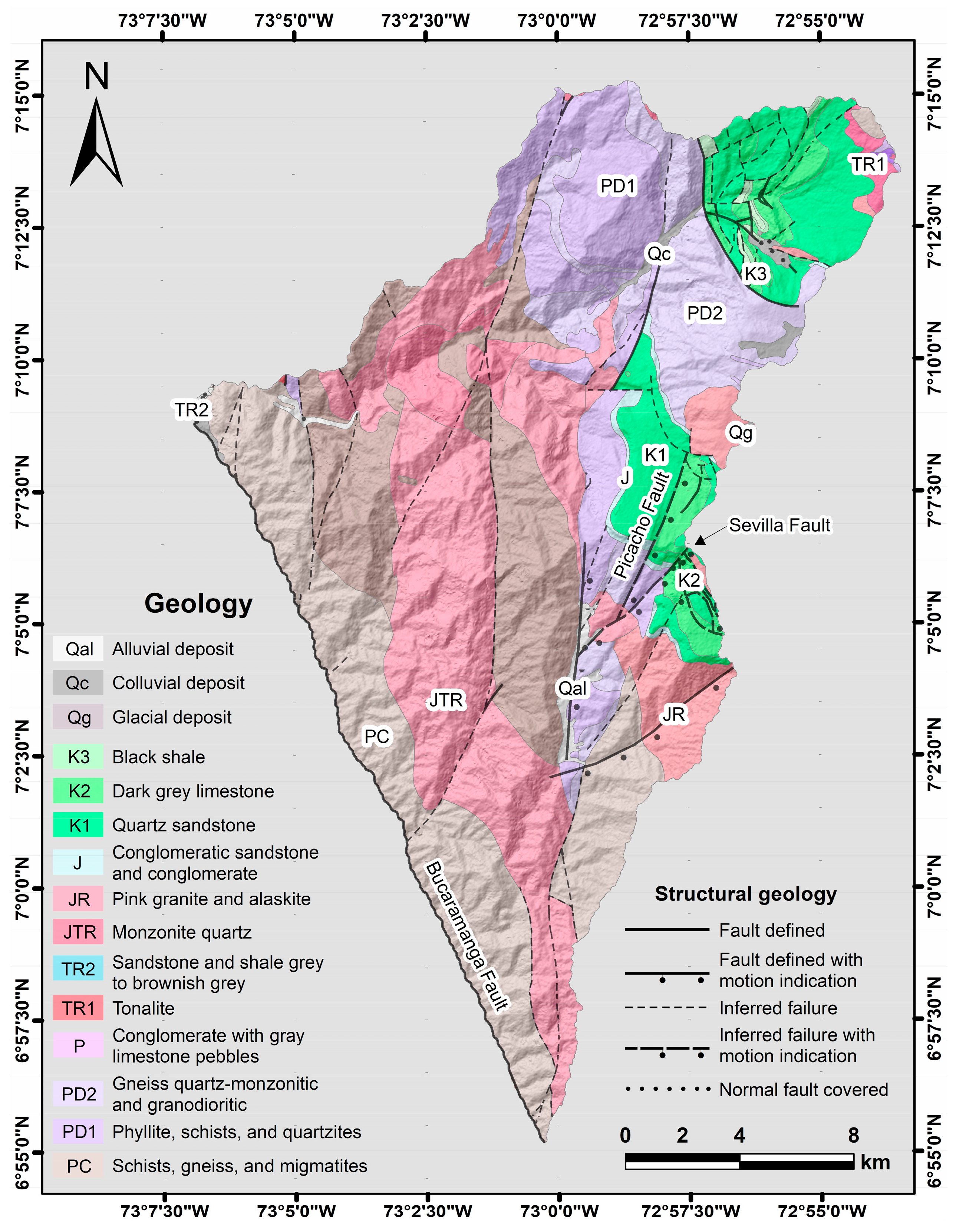
2. Regional Setting
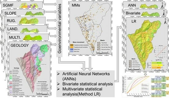
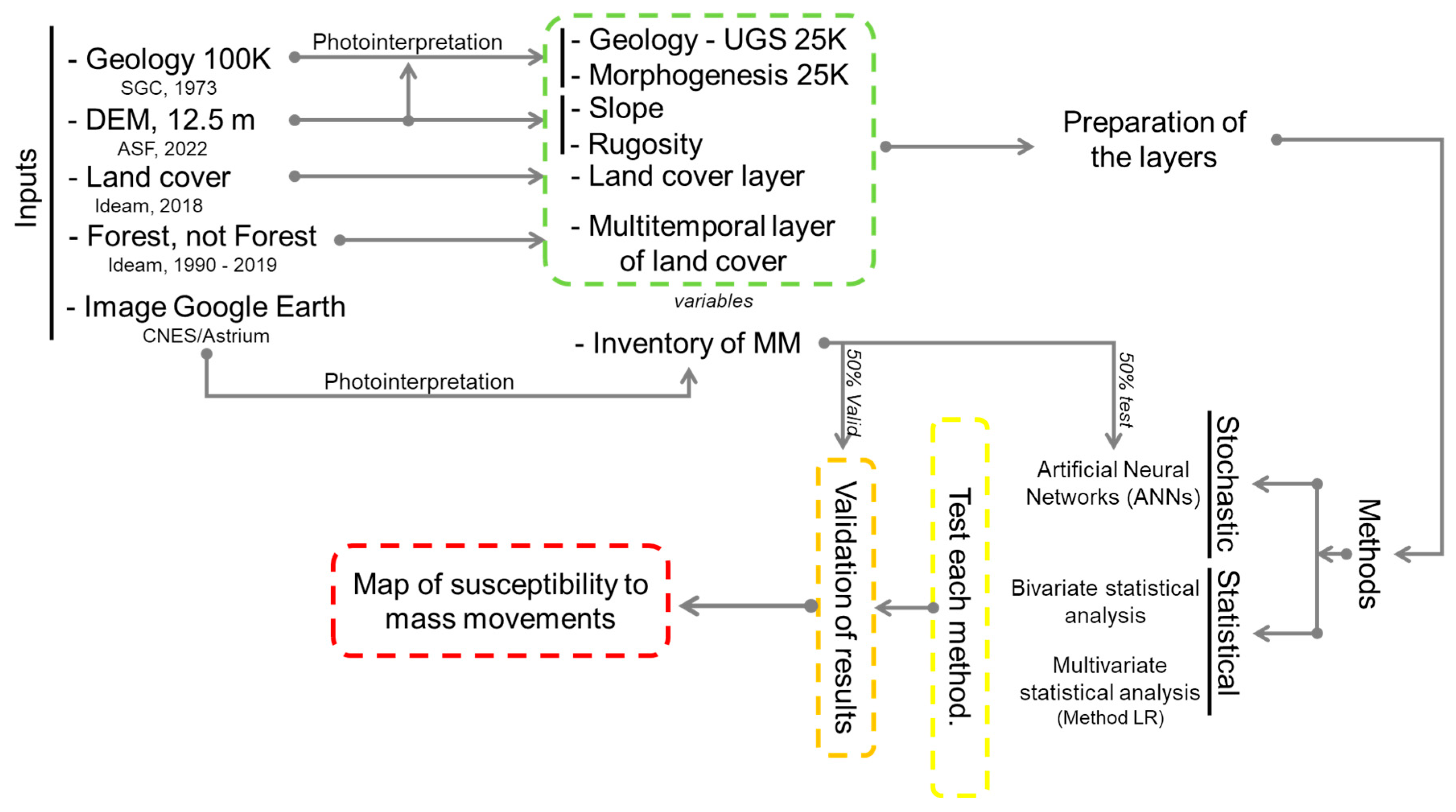
3. Methodology and Materials
3.1. Construction of Inherent and Dependent Variables
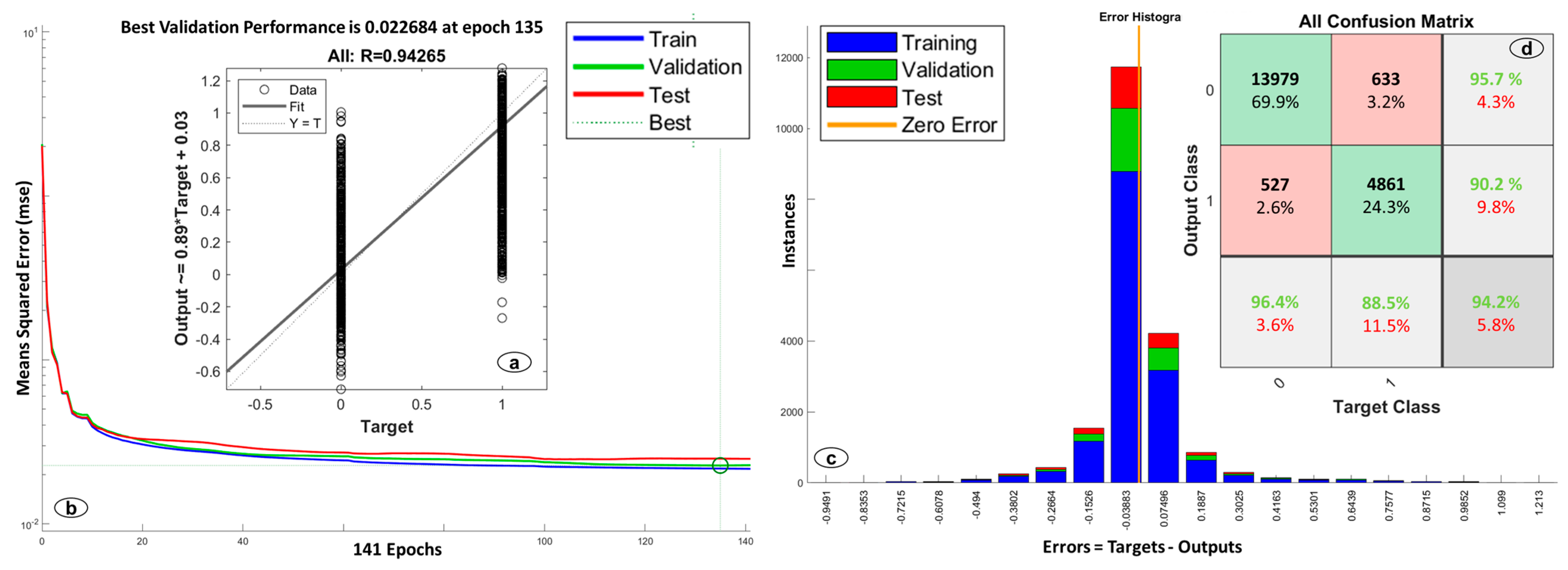
3.2. Methods for Calculating Susceptibility by Mass Movements
3.3. Validation of the Susceptibility Model
4. Results
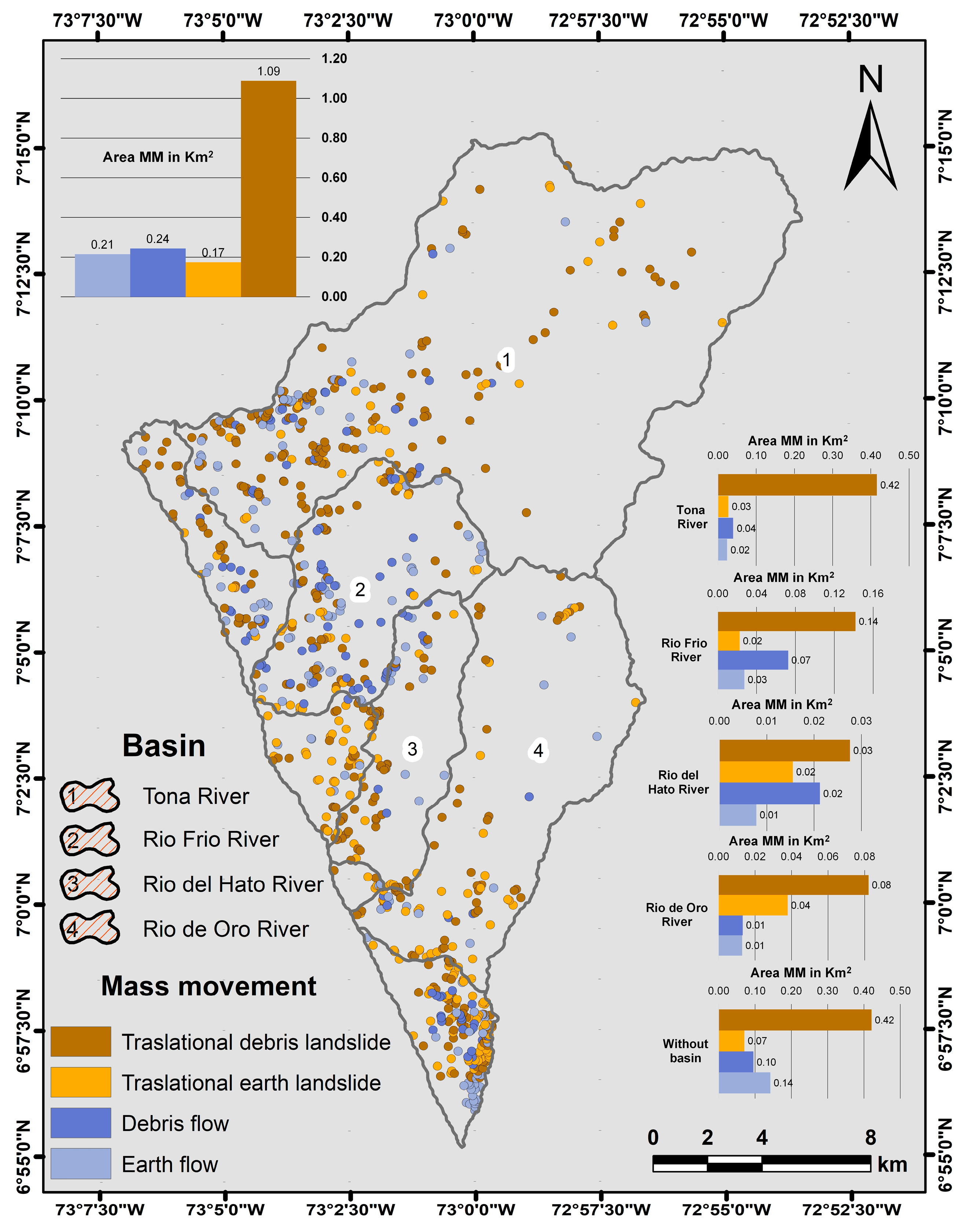
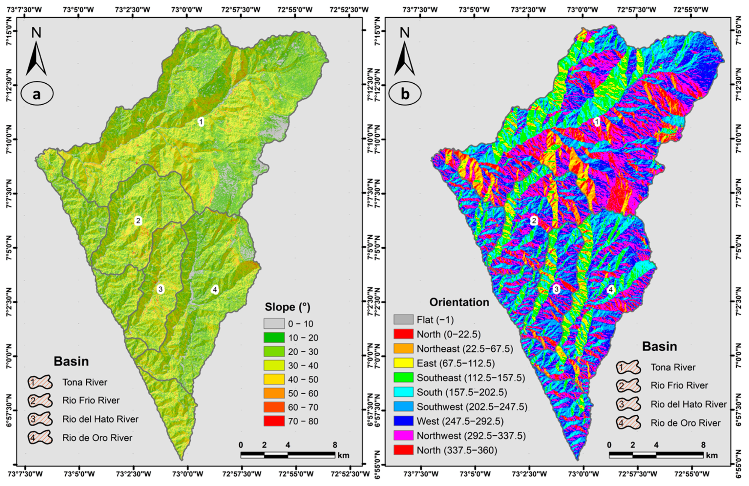
4.1. Description of Geoenvironmental Elements
- Selection of MM randomly;
- Randomly selected MMs should have equivalent areas in both test and validation;
- The MMs must be spatially distributed;
- Within 50% of each selection, you must have 25% of each type of MM described (4 types of MM).
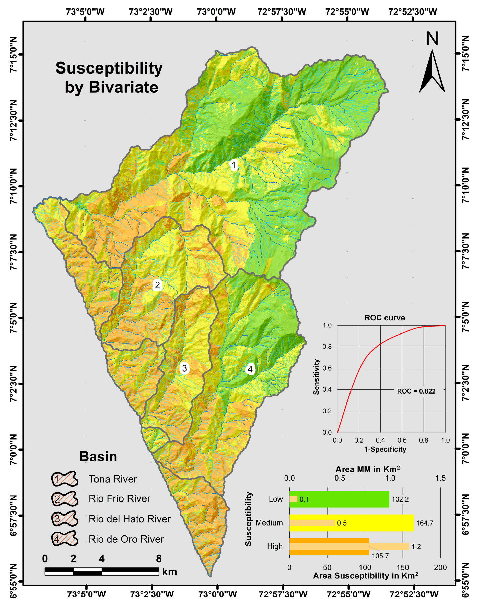
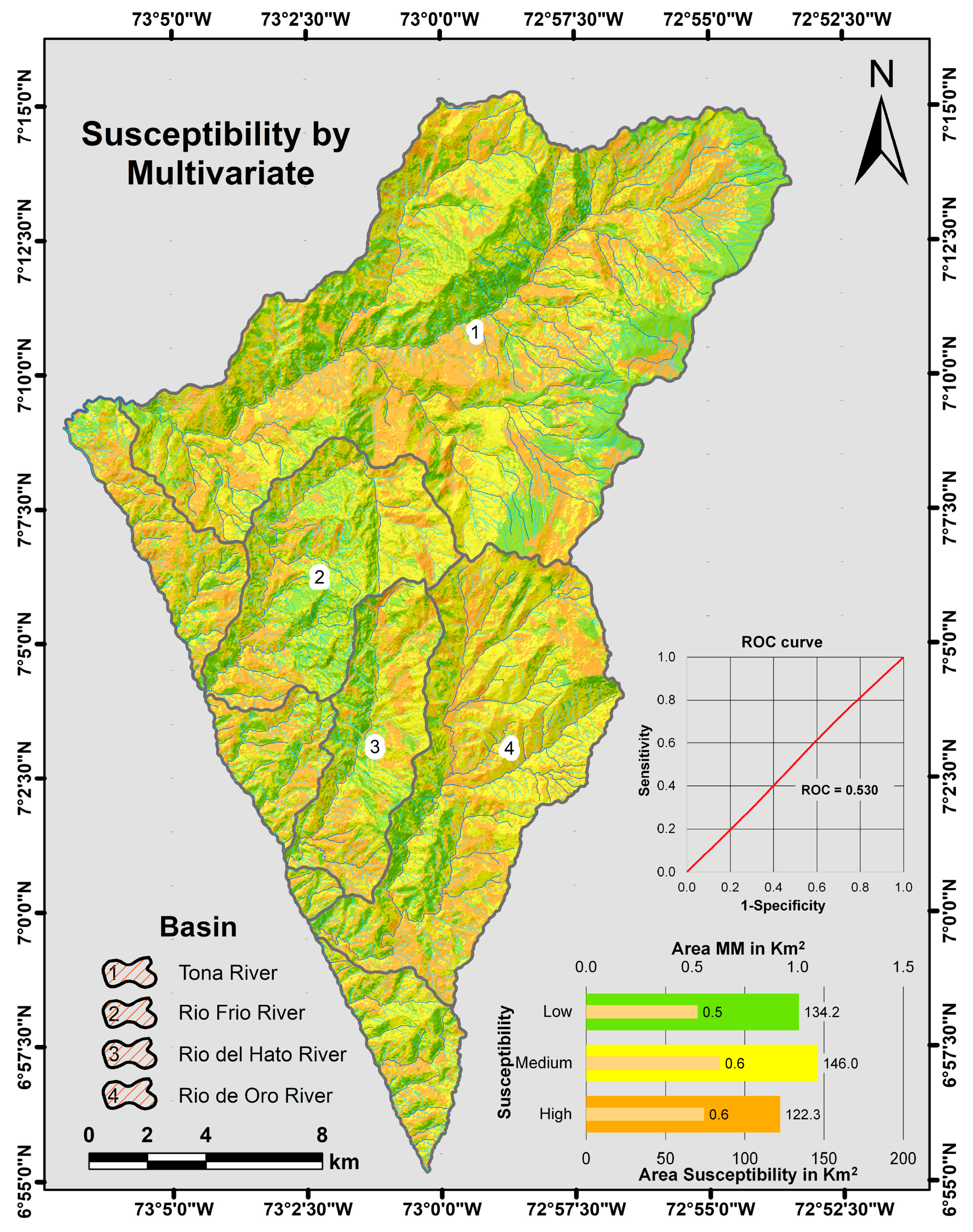
4.2. Calculation of Susceptibility
5. Discussion
- The results obtained from the susceptibility calculation carried out in each basin have a prediction greater than 70% (AUC curve) in the test phase. This demonstrates a good development in the spatial prediction of regions with different susceptibility ranges. As it is also appreciated that the AUC curves of the validation present a percentage higher than 60%, indicating that the areas with the events that were not included in the calculation of the test were classified correctly;
- Within the calculation of susceptibility and taking into consideration the results obtained from the AUC curves, a condition can be established in the construction of the inherent variables, which should not necessarily be restricted to the geometry of the hydrographic basin. Since, generally, susceptibility models are limited to this geometry. From the analysis carried out in the present study, the regions of the model can be expanded by duly safeguarding their limits in scale and level of interpretation. This can be established if you have your own knowledge of the region evaluated and experience in the field of study (expert criteria). As well, if variables such as geology, geomorphology, and land cover, do not present a change of more than 20% in their attributes over the areas that enter the calculation of the susceptibility model;
- From the present study, it is also indicated that the hydrographic basins that have a surface area less than 50 km2 do not generate an ideal model of susceptibility. In these cases, it is convenient to make a model with a greater extension. But with the dimension that must be considered with those described in the previous point and the calculation must be performed with the algorithm of bivariate statistical analysis.
6. Conclusions
Author Contributions
Funding
Data Availability Statement
Acknowledgments
Conflicts of Interest
References
- World Health Organization. Landslides. 2019. Available online: https://www.who.int/health-topics/landslides#tab=tab_1 (accessed on 25 June 2022).
- EM-DAT. Centre for Research on the Epidemiology of Disasters. Available online: https://www.emdat.be/ (accessed on 25 June 2022).
- Froude, M.; Petly, D. Global Fatal Landslide Ocurrencen 2004 to 2016. Nat. Hazards Earth Syst. Sci. Discuss. 2018, 18, 2161–2181. [Google Scholar] [CrossRef]
- SGC. Guía Metodológica para la Zonificación de Amenaza por Movimientos en Masa Escala 1:25.000; Servicio Geológico Colombiano: Bogota, Colombia, 2017. [Google Scholar]
- DesInventar.org. Disaster Information Management System. Available online: https://www.desinventar.org/ (accessed on 10 April 2022).
- Ingeominas. Catálogo nacional de movimientos en masa. In Subdirección de Amenazas Geoambiéntales; Ingeominas: Bogotá, Colombia, 2002. [Google Scholar]
- SGC. Las amenazas por movimientos en masa de Colombia, una visión a escala 1:100.000. In Grupo de Evaluación de Amenaza por Movimientos en Masa; Servicio Geológico Colombiano: Bogotá, Colombia, 2017. [Google Scholar] [CrossRef]
- Cruden, D.M. A simple definition of a landslide. Bull. Int. Assoc. Eng. Geol. 1991, 43, 27–29. [Google Scholar] [CrossRef]
- Popescu, M. Landslide Causal Factors and Landslide Remedial Options. In Proceedings of the 3rd International Conference on Landslides, Slope Stability and Safety of Infra-Structures, Singapore, 11–12 July 2002; pp. 61–81. [Google Scholar]
- van Westen, C.J.; Castellanos, E.; Kuriakose, S.L. Spatial data for landslide susceptibility, hazard, and vulnerability assessment: An overview. Eng. Geol. 2008, 102, 112–131. [Google Scholar] [CrossRef]
- Liang, L.; Tao, C.; Jie, D.; Antonio, P. A hybrid ensemble-based deep-learning framework for landslide susceptibility mapping. Int. J. Appl. Earth Obs. Geoinf. 2022, 108, 102713. [Google Scholar] [CrossRef]
- Fell, R.; Corominas, J.; Bonnard, C.; Cascini, L.; Leroi, E.; Savage, W. Guidelines for landslide susceptibility, hazard and risk zoning for land-use planning, on behalf of the JTC-1 Joint Technical Committee on Landslides and Engineered Slopes. Eng. Geol. 2008, 102, 85–98. [Google Scholar] [CrossRef]
- Martinez-Graña, A.M.; Goy, J.L.; Zazo, C. Geomorphological applications for susceptibility mapping of landslides in natural parks. Environ. Eng. Manag. J. 2016, 2, 15. [Google Scholar] [CrossRef]
- Rui, L.; YueKai, D.; Deliang, S.; Haijia, W.; Qingyu, G.; Shuxian, S.; Mingyong, L. Insights into spatial differential characteristics of landslide susceptibility from sub-region to whole-region cased by northeast Chongqing, China. Geomat. Nat. Hazards Risk 2023, 14, 25. [Google Scholar] [CrossRef]
- Soeters, R.; van Westen, C.J. Slope instability recognition, analysis and zonation. In Landslide Types and Processes; Special Report; Turner, A.K., Schuster, R.L., Eds.; National Research Council 247, National Academy of Sciences: Washington, DC, USA, 1996; Volume 247, pp. 129–177. [Google Scholar]
- Huanga, F.; Cao, Z.; Guo, J.; Jiang, S.; Li, S.; Guo, Z. Comparisons of heuristic, general statistical and machine learning models for landslide susceptibility prediction and mapping. Catena 2020, 191, 104580. [Google Scholar] [CrossRef]
- Cascini, L. Applicability of landslide susceptibility and hazard zoning at different scales. Eng. Geol. 2008, 102, 164–177. [Google Scholar] [CrossRef]
- Ingeominas. Zonificación Sismogeotécnica Indicativa del Área Metropolitana de Bucaramanga; Ingeominas, Subdirección de Amenazas Geoambientales: Bogotá, Colombia, 2001. [Google Scholar]
- UNDRR. Sendai framework for Disaster Risk Reduction 2015–2030. In United Nations (ONU); United Nations Office for Disaster Risk Reduction: Geneva, Switzerland, 2015. [Google Scholar]
- IDEAM. Geoportal—IDEAM. Consulta y Descarga de Datos Hidrometeorológicos. Available online: http://dhime.ideam.gov.co/atencionciudadano/ (accessed on 5 April 2022).
- Ward, D.E.; Goldsmith, R.; Jimeno, A.; Cruz, J.; Restrepo, H.; Gómez, E. Mapa geológico de Colombia, cuadrángulo h-12 Bucaramanga. Planchas 109 Rionegro—120 Bucaramanga. Cuadrángulo H-13 Pamplona. In Planchas 110 Pamplona—121Cerrito; Ingeominas: Bogotá, Colombia, 1973. [Google Scholar]
- Velandia, F.; Bermúdez, M. The transpressive southern termination of the Bucaramanga fault (Colombia): Insights from geological mapping, stress tensors, and fractal analysis. J. Struct. Geol. 2018, 115, 190–207. [Google Scholar] [CrossRef]
- Siravo, G.; Fellin, M.G.; Faccena, C.; Maden, C. Transpression and the build-up of the Cordillera: The example of the Bucaramanga fault (Eastern Cordillera, Colombia). J. Geol. Soc. 2020, 177, 14–30. [Google Scholar] [CrossRef]
- Osorio Naranjo, J.A.; Hernández Moreno, C.; Torres Jaimes, E.M.; Botero Santa, P.A.; Diederix, H. Modelo Geodinámico del Macizo de Santander; Ingeominas: Bogotá, Colombia, 2008. [Google Scholar]
- IGAC. Agustín Codazzi Geographical Institute. Open Data. Available online: https://geoportal.igac.gov.co/contenido/datos-abiertos-cartografia-y-geografia (accessed on 9 April 2022).
- ASF, A.P. Alaska Satellite Facility. Dataset: ASF DAAC 2015, ALOS PALSAR_Radiometric_Terrain_Corrected_Low_Res. Available online: https://asf.alaska.edu/data-sets/derived-data-sets/alos-palsar-rtc/alos-palsar-radiometric-terrain-correction/ (accessed on 9 April 2022).
- Servicio Geológico Colombiano (SGC). Estado de la Cartografía Geológica. Available online: http://srvags.sgc.gov.co/Flexviewer/Estado_Cartografia_Geologica/ (accessed on 9 April 2022).
- Instituto de Hidrología, Meteorología y Estudios Ambientales (IDEAM). Open Data Geographic Information. Find File: Land Cover. Available online: http://www.ideam.gov.co/capas-geo (accessed on 9 April 2022).
- Instituto de Hidrología, Meteorología y Estudios Ambientales (IDEAM). Open Data Geographic Information. Find File: Forest, Not Forest. Available online: http://www.ideam.gov.co/web/guest/galeria-de-mapas (accessed on 9 April 2022).
- Selby, M.J. Hillslope Materials and Processes, 2nd ed.; Oxford University Press: Oxford, UK, 1993. [Google Scholar]
- Kanki, M.A. Critical issues in soft rocks. J. Rock Mech. Geotech. Eng. 2014, 6, 186–195. [Google Scholar] [CrossRef]
- Hermelín, M. Suelos, Rocas y Formaciones Superficiales. DYNA 1985, 106, 25–29. [Google Scholar]
- Verstappen, H. Geomorfología Aplicada al Estudio de los Riesgos Naturales; Apuntes de Clase ITC: Holanda, The Netherlands, 1987. [Google Scholar]
- Carvajal, J.H. Primeras Aproximaciones a la Estandarización de la Geomorfología en Colombia; Instituto Colombiano de Geología y Minería: Bogotá, Colombia, 2008. [Google Scholar]
- Carvajal, J.H. Propuesta de Estandarización de la Cartografía Geomorfológica en Colombia; Servicio Geológico Colombiano: Bogotá, Colombia, 2012. [Google Scholar]
- Carvajal, J.H. Caracterización de la metodología geomorfológica adaptada por ingeominas. In Documento Interno Sometido a Discusión y Modificaciones; Instituto Colombiano de Geología y Minería: Bogotá, Colombia, 2002. [Google Scholar]
- Zinck, J.A. Geopedología: Elementos de Geomorfología para Estudios de Suelos y de Riesgos Naturales. In Enschede: International Institute for Geo-Information Science and Earth Observation (ITC); ITC Special Lecture Notes Series; University of Twente: Enschede, The Netherlands, 2012. [Google Scholar]
- Pike, R.J. Geomorphometry: Progress, pratice, and prospect. Z. Geomorphol. Suppl. 1995, 101, 221–238. [Google Scholar]
- Gallant, J.C.; Hutchinson, M.F. Digital terrain analysis. In Guidelines for Surveying Soil and Land Resources; McKenzie, N.J., Grundy, M.J., Ringrose-Voase, R.W.A.J., Eds.; Australian Soil and Land Survey Handbook Series; CSIRO: Melbourne, Australia, 2008; Volume 2. [Google Scholar]
- Olaya, V. Chapter 6 Basic Land-Surface Parameters. Dev. Soil Sci. 2009, 33, 141–169. [Google Scholar] [CrossRef]
- Wilson, J.; Gallant, J. Terrain Analysis: Principles and Applications; John Wiley & Sons, Inc.: Wiley, NY, USA, 2000. [Google Scholar]
- Saha, A.K.; Gupta, R.P.; Sarkar, I.; Arora, M.K.; Csaplovics, E. An approach for GIS-based statistical landslide susceptibility zonation—With a case study in the Himalayas. Landslides 2005, 2, 61–69. [Google Scholar] [CrossRef]
- Yalcin, A.; Reis, S.; Aydinoglu, A.; Yomralioglu, T. A GIS-based comparative study of frequency ratio, analytical hierarchy process, bivariate statistics and logistics regression methods for landslide susceptibility mapping in Trabzon, NE Turkey. Catena 2011, 85, 274–287. [Google Scholar] [CrossRef]
- Santacana, N. Análisis de la susceptibilidad del terreno a la formación de deslizamientos superficiales y grandes deslizamientos mediante el uso de sistemas de información geográfica. In Aplicación a la Cuenca Alta del río Llobregat; Tesi Doctoral, UPC; Departament d’Enginyeria del Terreny, Cartogràfica i Geofísica: Barcelona, Spain, 2001. [Google Scholar]
- Felicisimo, A.M. Modelos Digitales del Terreno; Pentalfa: Oviedo, Spain, 1994; Available online: http://www.etsimo.uniovi.es/~feli (accessed on 16 November 2016).
- Corominas, J.; Van Westen, C.; Frarrini, P.; Cascini, L.; Malet, J.P.; Fotopoulou, S.; Smith, J.T. Recommendations for the quantitative analysis of landslide risk. Bull. Eng. Geol. Environ. 2014, 73, 209–263. [Google Scholar] [CrossRef]
- Sato, H.P.; Harp, E.L. Interpretation of earthquake-induced landslides triggered by the 12 May 2008, M7. 9 Wenchuan earthquake in the Beichuan area, Sichuan Province, China using satellite imagery and Google Earth. Landslides 2009, 6, 153–159. [Google Scholar] [CrossRef]
- Guzzetti, F.; Mondini, A.C.; Cardinali, M.; Fiorucci, F.; Santangelo, M.; Chang, K. Landslide inventory maps: New tools for an old problem. Earth-Sci. Rev. 2012, 112, 42–66. [Google Scholar] [CrossRef]
- Varnes, D.J. Slope movement types and processes. In Landslides: Analysis and Control; Schuster, R.L., Krizek, R.J., Eds.; Transportation and Road Research Board, National Academy of Science: Washington, DC, USA, 1978; pp. 11–33. [Google Scholar]
- PMA-GCA. Proyecto Multinacional Andino (PMA): Geociencias para las Comunidades Andinas (GCA). In Movimientos en Masa en la Región Andina: Una Guía para la Evaluación de Amenazas; Publicación Geológica Multinacion, Servicio Nacional de Geología y Minería: 2007; 2007. [Google Scholar]
- Hungr, O.; Leroueil, S.; Picarelli, L. The Varnes classification of landslide types, an update. Landslides 2014, 11, 167–194. [Google Scholar] [CrossRef]
- Skemton, A.W.; Hutchinson, J.N. Stability of natural slopes and embankment foundations. In Proceedings of the Seventh lntemational Conference on Soil Mechanics and Foundation Engineering 4; Sociedad Mexicana de Mecánica de de Suelos: México City, Mexico, 1969; pp. 291–340. Available online: https://trid.trb.org/view/125702 (accessed on 7 April 2022).
- Bossard, M.; Feranec, J.; Otahel, J. CORINE Land Cover Technical Guide: Addendum 200; European Environment Agency: Copenhagen, Denmark, 2000; Volume 40. [Google Scholar]
- Charman, P.V.; Murphy, B.W. Soils: Their Properties and Management, 2nd ed.; Melbourne y Oxford; Oxford University Press: Oxford, UK, 2000. [Google Scholar]
- Suárez, N.J. Deslizamientos y Estabilidad de Taludes en Zonas Tropicales; Universidad Industrial de Santander: Bucaramanga, Colombia, 1998. [Google Scholar]
- Mugagga, F.; Kakembo, V.; Buyinza, M. Land use changes on the slopes of Mount Elgon and the implications for the occurrence of landslides. Catena 2012, 90, 39–46. [Google Scholar] [CrossRef]
- UN. United Nations—Climate Change. Available online: https://unfccc.int/topics/land-use/resources/redd-documents (accessed on 13 April 2022).
- Csiszar, I.A.; Justice, C.O.; Goldammer, J.G.; Lynham, T.; Groot, W.D.; Prins, E.M.; Stephens, G. The GOFC-GOLD fire mapping and monitoring theme: Assessment and strategic plans. In Remote Sensing and Modeling Applications to Wildland Fires; Springer: Berlin/Heidelberg, Germany, 2013; pp. 341–372. [Google Scholar] [CrossRef]
- Feranec, J.; Jaffrain, G.; Soukup, T.; Hazeu, G. Determining changes and flows in European landscapes 1990–2000 using CORINE land cover data. Appl. Geogr. 2010, 30, 19–35. [Google Scholar] [CrossRef]
- Reichenbach, P.; Busca, C.; Mondini, A.C.; Rossi, M. The Influence of Land Use Change on Landslide Susceptibility Zonation: The Briga Catchment Test Site (Messina, Italy). Environ. Manag. 2014, 54, 1372–1384. [Google Scholar] [CrossRef]
- Van Beek, L.H.; Van Asch, T.J. Regional assessment of the effects of land-use change and landslide hazard by means of physically based modeling. Nat. Hazards 2004, 30, 289–304. [Google Scholar] [CrossRef]
- Pisano, L.; Zumpano, V.; Malek, Ž.; Rosskopf, C.M.; Parise, M. Variations in the susceptibility to landslides, as a consequence of land cover changes: A look to the past, and another towards the future. Sci. Total Environ. 2017, 601, 1147–1159. [Google Scholar] [CrossRef]
- Guzzetti, F.; Carrara, A.; Cardinali, M.; Reichenbach, P. Landslide hazard evaluation: A review of current techniques and their application in a multi-scale study, Central Italy. Geomorphology 1999, 31, 181–216. [Google Scholar] [CrossRef]
- Gardiner, C.W. Handbook of Stochastic Methods; Springer: Berlin, Germany, 1985; Volume 3. [Google Scholar]
- Barrera, D. Modelos Deterministicos y Probabilisticos; Universidad José María Vargas: Caracas, Venezuela, 2016. [Google Scholar]
- Simpson, P.K. Artificial Neural System—Foundation, Paradigm, Application and Implementation; Pergamon Press: New York, NY, USA, 1990. [Google Scholar]
- Anderson, D.; McNeill, G. Artificial Neural Networks Technology; Kaman Sciences Corporation: Bloomfield, CT, USA, 1992. [Google Scholar]
- De Brio, B.; Sanz, A. Redes Neuronales y Srosos; Alfaomega: México, México, 2007. [Google Scholar]
- Pradhan, B.; Lee, S.; Buchoithner, M.F. A GIS-based back-propagation neural network model and its cross-application and validation for landslide susceptibility analyses. Comput. Environ. Urban Syst. 2010, 34, 216–235. [Google Scholar] [CrossRef]
- Lee, S.; Park, I.; Choi, J.K. Spatial prediction of ground subsidence susceptibility using an artificial neural network. Environ. Manag. 2012, 49, 347–358. [Google Scholar] [CrossRef]
- Valencia Ortiz, J.A.; Martínez-Graña, A.M. A neural network model applied to landslide susceptibility analysis (Capitanejo, Colombia). Geomat. Nat. Hazards Risk 2018, 9, 1106–1128. [Google Scholar] [CrossRef]
- Bonham-Carter, G.F.; Agterberg, F.P.; Wright, D.F. Integration of geological datasets for gold exploration in Nova Scotia. Photogramm. Eng. Remote Sens. 1988, 54, 1585–1592. [Google Scholar] [CrossRef]
- Bonham, G. Geographic Information Systems for Geoscientists: Modelling with GIS (No. 13); Pergamon, Ed.; Elsevier: Amsterdam, The Netherlands, 1994; Volume 13. [Google Scholar]
- van Westen, C. Guidelines for the Generation of 1:50.000 Scale Landslide Inventory, Susceptibility Maps, and Qualitative Risk Maps, Illustrated with Case Studies of the Provinces Thanh Hoa and Nghe An; University of Twente: Enschede, The Netherlands, 2013. [Google Scholar]
- Chen, W.; Chai, H.; Sun, X.; Wang, Q.; Ding, X.; Hong, H. A GIS-based comparative study of frequency ratio, statistical index and weights-of-evidence models in landslide susceptibility mapping. Arab. J. Geosci. 2016, 9, 204. [Google Scholar] [CrossRef]
- Kendall, M.G. Multivariate Analysis; Griffin: London, UK, 1975. [Google Scholar]
- Carrara, A.; Cardinali, M.; Detti, R.; Guzzetti, F.; Pasqui, V.; Reichenbach, P. GIS techniques and statistical models in evaluating landslide hazard. Earth Surf. Proc. Land 1991, 16, 427–445. [Google Scholar] [CrossRef]
- Bernknopf, R.; Cambell, R.; Brookshire, D.; Shapiro, C. A probabilistic approach to landslide hazard mapping in Cincinnati, Ohio, with applications for economic evaluation. Bull Int. Assoc. Eng. Geol. 1988, 25, 39–56. [Google Scholar] [CrossRef]
- Fiuza, P.D.; Rodríguez, P.J. La regresión logística: Una herramienta versátil. Nefrologia 2000, 20, 495–500. [Google Scholar]
- Baeza, C.; Corominas, J. Assessment of shallow landslide susceptibility by means of multivariate statistical techniques. Earth Surface Processes and Landforms. J. Br. Geomorphol. Res. Group 2001, 26, 1251–1263. [Google Scholar] [CrossRef]
- Kavzoglu, T.; Kutlug, S.E.; Colkesen, I. An assessment of multivariate and bivariate approaches in landslide susceptibility mapping: A case study of Duzkoy district. Nat. Hazards 2015, 76, 471–496. [Google Scholar] [CrossRef]
- Gómez, N.F.; Mendez, L.M.; Valencia Ortiz, J.A. Zonificación de la susceptibilidad por movimientos en masa, escala 1:10.000 para el municipio de Suratá, Santander, aplicando métodos estadísticos multivariables (regresión logística). In Trabajo de Grado; Universidad Industrial de Santander: Bucaramanga, Colombia, 2017. [Google Scholar]
- Lee, S.; Pradhan, B. Landslide hazard mapping at Selangor, Malaysia using frecuency ratio and logistic regression models. Landslides 2007, 4, 33–41. [Google Scholar] [CrossRef]
- Aguayo, M. Como Hacer una Regresión Logística con SPSS “Paso a Paso” (I). Available online: http://metodos-avanzados.sociales.uba.ar/wp-content/uploads/sites/216/2014/03/Regres_log_AGUAYO-otros.pdf (accessed on 16 April 2022).
- Aguayo, M.; Lora, E. Como Hacer una Regresión Logística Binaria “Paso a Paso” (II): Análisis Multivariante. Available online: https://documentop.com/como-hacer-una-regresion-logistica-binaria-fabis_5a0eb71e1723dd59aa821c5b.html (accessed on 16 April 2022).
- Dahal, R.K.; Hasegawa, S.; Nonomura, A.; Yamanaka, M.; Dhakal, S.; Paudyal, P. Predictive modelling of rainfall-induced landslide hazard in the Lesser Himalaya of Nepal based on weights-of-evidence. Geomorphology 2008, 102, 496–510. [Google Scholar] [CrossRef]
- Vakhshoori, V.; Zare, M. Landslide susceptibility mapping by comparing weight of evidence, fuzzy logic, and frequency ratio methods. Geomat. Nat. Hazards Risk 2016, 7, 1731–1752. [Google Scholar] [CrossRef]
- Salitchev, K.A. Cartografía; Pueblo y Educación: La Habana, Cuba, 1979. [Google Scholar]
- Verstappen, H.T.; van Zuidam, R.A. The ITC System of Geomorphological Survey; ITC Publication Number 10; ITC: Enschede, The Netherlands, 1992. [Google Scholar]
- van Zuidam, R.A. Aerial Photointerpretation in Terrain Analysis and Geomorphological Mapping; Smiths Publishers: Tha Hague, The Netherlands, 1986. [Google Scholar]
- Cruden, D.M.; Varnes, D.J. Landslide Types and Processes. Special Report. In Lanslides: Investigation and Mitigation; Turner, A.K., Schuster, R.L., Eds.; National Research Council 247; National Academy of Sciences: Washington, DC, USA, 1996; pp. 36–75. [Google Scholar]
- IDEAM. Monitoreo de la Superficie Cubierta por Bosque Natural. Available online: http://www.ideam.gov.co/web/ecosistemas/superficie-cubierta-por-bosque-natural?inheritRedirect=true (accessed on 13 April 2022).
- Li, Y.; Mo, P. A unified landslide classification system for loess slopes: A critical review. Geomorphology 2019, 340, 67–83. [Google Scholar] [CrossRef]
- Valencia Ortiz, J.A.; Martínez-Graña, A.M. Morphometric Evaluation and Its Incidence in the Mass Movements Present in the Chicamocha Canyon, Colombia. Sustainability 2023, 15, 1140. [Google Scholar] [CrossRef]
- Bathrellos, G.D.; Gaki-Papanastassiou, K.; Skilodimou, H.D.; Papanastassiou, D.; Chousianitis, K.G. Potential suitability for urban planning and industry development using natural hazard maps and geological–geomorphological parameters. Environ. Earth Sci. 2012, 66, 537–548. [Google Scholar] [CrossRef]
- Valencia Ortiz, J.A.; Martínez-Graña, A.M. Calculation of precipitation and seismicity thresholds as triggers for mass movements in the region of Bucaramanga, Colombia. Ecol. Indic. 2023, 152, 110355. [Google Scholar] [CrossRef]


| Ranking Classification | ||||||
|---|---|---|---|---|---|---|
| Count | Area km2 | Min | Max | Range | Mean | Std |
| 10,982 | 1.715 | 0° | 74.897° | 74.897° | 31.42936° | 9.7631 |
| Slope | ||||||
| Range | Without MM | With MM | ||||
| Count | Area km2 | % | Count | Area km2 | % | |
| 0–10° | 167,861 | 26.23 | 6.52 | 201 | 0.03 | 1.83 |
| 10–20° | 595,628 | 93.07 | 23.12 | 1072 | 0.17 | 9.76 |
| 20–30° | 937,852 | 146.54 | 36.40 | 3457 | 0.54 | 31.48 |
| 30–40° | 662,061 | 103.45 | 25.70 | 4289 | 0.67 | 39.05 |
| 40–50° | 183,423 | 28.66 | 7.12 | 1632 | 0.26 | 14.86 |
| 50–60° | 25,379 | 3.97 | 0.99 | 291 | 0.05 | 2.65 |
| 60–70° | 3865 | 0.60 | 0.15 | 39 | 0.01 | 0.36 |
| >70° | 236 | 0.04 | 0.01 | 1 | 0.00 | 0.01 |
| Basin | Susceptibility by MM | Quantity of MM per Category | ||||||||||
|---|---|---|---|---|---|---|---|---|---|---|---|---|
| Low | % | Medium | % | High | % | Low | % | Medium | % | High | % | |
| Tona | 383,500 | 30.5 | 547,711 | 43.5 | 326,806 | 26.0 | 217 | 6.7 | 1303 | 40.1 | 1726 | 53.2 |
| Río Frio | 9070 | 3.1 | 114,284 | 39.1 | 169,138 | 57.8 | 34 | 2.0 | 697 | 42.0 | 930 | 56.0 |
| Rio del Hato | 19,812 | 10.0 | 108,577 | 54.6 | 70,581 | 35.5 | 42 | 10.2 | 186 | 45.0 | 185 | 44.8 |
| Rio de Oro | 77,552 | 15.6 | 210,294 | 42.3 | 209,127 | 42.1 | 37 | 4.2 | 359 | 40.6 | 489 | 55.3 |
| W/B | 56,146 | 16.6 | 165,165 | 48.9 | 116,590 | 34.5 | 251 | 5.2 | 1425 | 29.8 | 3105 | 64.9 |
| Basin | Susceptibility by MM | Quantity of MM per Category | ||||||||||
|---|---|---|---|---|---|---|---|---|---|---|---|---|
| Low | % | Medium | % | High | % | Low | % | Medium | % | High | % | |
| Tona | 637,558 | 50.8 | 441,655 | 35.2 | 174,785 | 13.9 | 423 | 13.0 | 1136 | 35.0 | 1684 | 51.9 |
| Río Frio | 3063 | 1.0 | 172,976 | 59.1 | 116,433 | 39.8 | 0 | 0.0 | 656 | 39.5 | 1005 | 60.5 |
| Rio del Hato | 1857 | 0.9 | 119,901 | 60.3 | 77,175 | 38.8 | 4 | 1.0 | 189 | 45.8 | 220 | 53.3 |
| Rio de Oro | 196,391 | 39.6 | 190,929 | 38.5 | 108,122 | 21.8 | 73 | 8.2 | 356 | 40.2 | 456 | 51.5 |
| W/B | 6957 | 2.1 | 128,350 | 38.3 | 199,664 | 59.6 | 0 | 0.0 | 544 | 11.4 | 4235 | 88.6 |
| Correlation | MM | LAND | TEM | PEN | RUG | UGS | |
|---|---|---|---|---|---|---|---|
| MM | Spearman correlation | 1.000 | |||||
| Sig. (bilateral) | |||||||
| N | 11,994 | ||||||
| LAND | Spearman correlation | −0.391 ** | 1.000 | ||||
| Sig. (bilateral) | 0.000 | ||||||
| N | 11,994 | 11,994 | |||||
| TEM | Spearman correlation | −0.289 ** | −0.046 ** | 1.000 | |||
| Sig. (bilateral) | 0.000 | 0.000 | |||||
| N | 11,994 | 11,994 | 11,994 | ||||
| PEN | Spearman correlation | 0.056 ** | −0.198 ** | −0.316 ** | 1.000 | ||
| Sig. (bilateral) | 0.000 | 0.000 | 0.000 | ||||
| N | 11,994 | 11,994 | 11,994 | 11,994 | |||
| RUG | Spearman correlation | 0.107 ** | −0.057 ** | −0.176 ** | 0.141 ** | 1.000 | |
| Sig. (bilateral) | 0.000 | 0.000 | 0.000 | 0.000 | |||
| N | 11,994 | 11,994 | 11,994 | 11,994 | 11,994 | ||
| UGS | Spearman correlation | −0.108 ** | 0.252 ** | 0.041 ** | −0.383 ** | −0.150 ** | 1.000 |
| Sig. (bilateral) | 0.000 | 0.000 | 0.000 | 0.000 | 0.000 | ||
| N | 11,994 | 11,994 | 11,994 | 11,994 | 11,994 | 11,994 | |
| Basin | Susceptibility by MM | Quantity of MM per Category | ||||||||||
|---|---|---|---|---|---|---|---|---|---|---|---|---|
| Low | % | Medium | % | High | % | Low | % | Medium | % | High | % | |
| Tona | 359,629 | 28.7 | 479,230 | 38.2 | 415,137 | 33.1 | 879 | 27.1 | 1240 | 38.2 | 1123 | 34.6 |
| Río Frio | 85,437 | 29.2 | 135,116 | 46.2 | 71,918 | 24.6 | 593 | 35.7 | 644 | 38.8 | 423 | 25.5 |
| Rio del Hato | 51,101 | 25.7 | 86,774 | 43.6 | 61,056 | 30.7 | 108 | 26.3 | 131 | 31.9 | 172 | 41.8 |
| Rio de Oro | 76,193 | 15.4 | 246,078 | 49.7 | 173,170 | 35.0 | 180 | 20.4 | 409 | 46.3 | 294 | 33.3 |
| W/B | 70,559 | 21.1 | 141,082 | 42.1 | 123,328 | 36.8 | 989 | 20.7 | 2612 | 54.7 | 1177 | 24.6 |
| Study Area | Basin | |||||
|---|---|---|---|---|---|---|
| Susceptibility | Area (km2) | % | Area (km2) | % | Variation (%) | |
| Low | 99.62 | 50.84 | 84.92 | 43.34 | −14.75 | |
| Tona River | Medium | 69.01 | 35.22 | 74.21 | 37.87 | 7.53 |
| High | 27.31 | 13.94 | 36.81 | 18.79 | 34.77 | |
| Total | 195.94 | 195.94 | ||||
| Low | 0.48 | 1.05 | 3.83 | 8.37 | 699.51 | |
| Río Frio River | Medium | 27.03 | 59.14 | 21.76 | 47.61 | −19.50 |
| High | 18.19 | 39.81 | 20.12 | 44.02 | 10.57 | |
| Total | 45.70 | 45.70 | ||||
| Low | 0.29 | 0.93 | 7.40 | 23.79 | 2448.73 | |
| Río del Hato River | Medium | 18.73 | 60.27 | 12.90 | 41.49 | −31.16 |
| High | 12.06 | 38.79 | 10.79 | 34.72 | −10.51 | |
| Total | 31.08 | 31.08 | ||||
| Low | 30.69 | 39.64 | 34.57 | 44.66 | 12.67 | |
| Río de Oro River | Medium | 29.83 | 38.54 | 24.81 | 32.05 | −16.85 |
| High | 16.89 | 21.82 | 18.03 | 23.29 | 6.74 | |
| Total | 77.41 | 77.41 | ||||
Disclaimer/Publisher’s Note: The statements, opinions and data contained in all publications are solely those of the individual author(s) and contributor(s) and not of MDPI and/or the editor(s). MDPI and/or the editor(s) disclaim responsibility for any injury to people or property resulting from any ideas, methods, instructions or products referred to in the content. |
© 2023 by the authors. Licensee MDPI, Basel, Switzerland. This article is an open access article distributed under the terms and conditions of the Creative Commons Attribution (CC BY) license (https://creativecommons.org/licenses/by/4.0/).
Share and Cite
Valencia Ortiz, J.A.; Martínez-Graña, A.M.; Méndez, L.M. Evaluation of Susceptibility by Mass Movements through Stochastic and Statistical Methods for a Region of Bucaramanga, Colombia. Remote Sens. 2023, 15, 4567. https://doi.org/10.3390/rs15184567
Valencia Ortiz JA, Martínez-Graña AM, Méndez LM. Evaluation of Susceptibility by Mass Movements through Stochastic and Statistical Methods for a Region of Bucaramanga, Colombia. Remote Sensing. 2023; 15(18):4567. https://doi.org/10.3390/rs15184567
Chicago/Turabian StyleValencia Ortiz, Joaquín Andrés, Antonio Miguel Martínez-Graña, and Lenny Mejía Méndez. 2023. "Evaluation of Susceptibility by Mass Movements through Stochastic and Statistical Methods for a Region of Bucaramanga, Colombia" Remote Sensing 15, no. 18: 4567. https://doi.org/10.3390/rs15184567
APA StyleValencia Ortiz, J. A., Martínez-Graña, A. M., & Méndez, L. M. (2023). Evaluation of Susceptibility by Mass Movements through Stochastic and Statistical Methods for a Region of Bucaramanga, Colombia. Remote Sensing, 15(18), 4567. https://doi.org/10.3390/rs15184567