4.1. Description of Geoenvironmental Elements
For this stage of processing the susceptibility model, a correct correlation and correspondence in scale and resolution must be obtained. According to Casini, [
17] the evaluation of susceptibility within a scheme of urban planning and zoning of regions may lead to a problem with anthropogenic factors that must be subject to large-scale cartographic elements. As well, it is relevant to establish a parameter of a minimum cartographic area that ensures a geometric construction relevant to the work scale, this is in order to ensure that the cartographic content of each variable preserves the criteria with which they were generated [
88]. To this end, a minimum cartographic area was defined for the 1:25,000 scale of 10,000 m
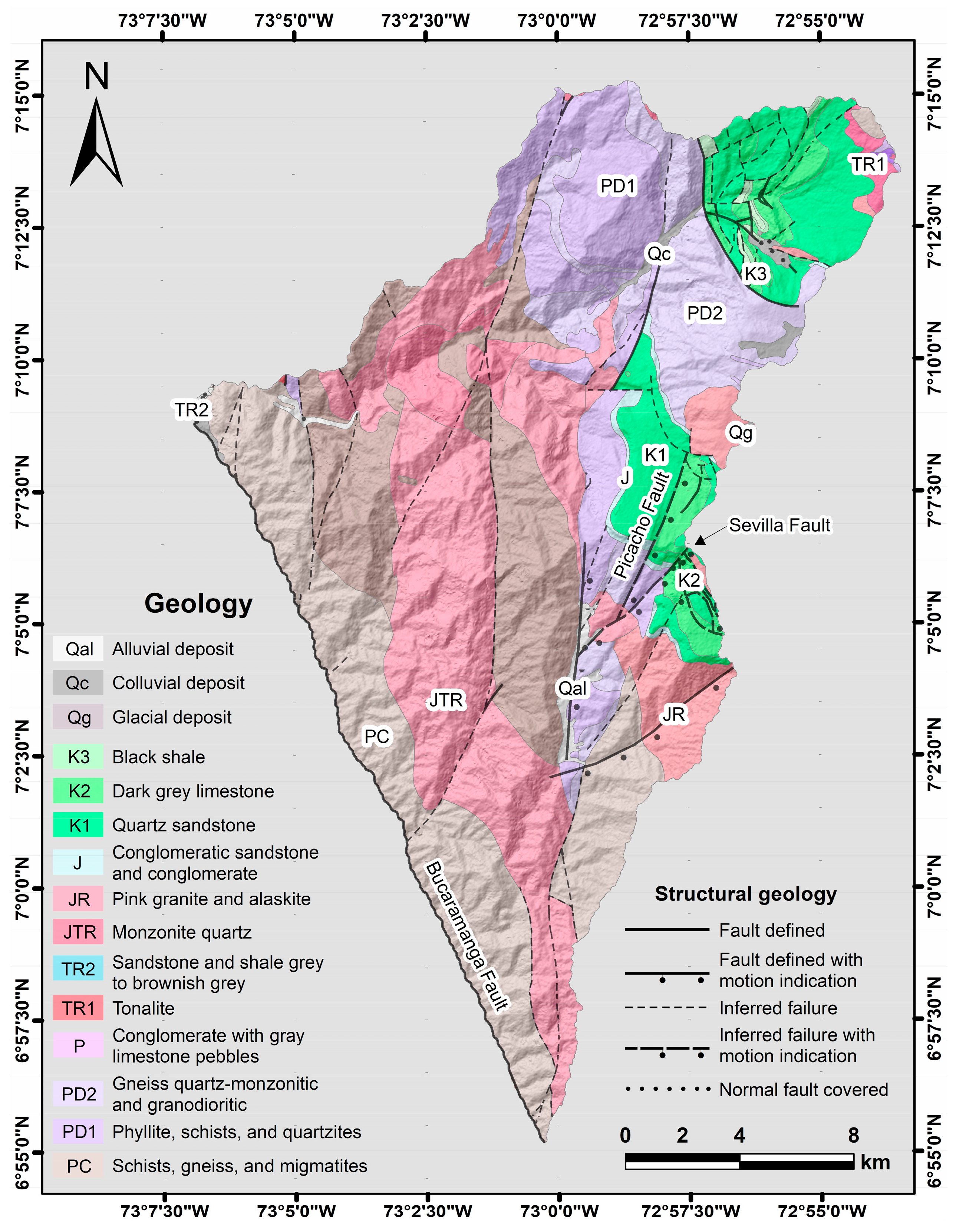
2 that is applied to each attribute generated for the variables of geology, morphogenesis, morphodynamics, and land cover. For the UGS variable, a cartographic adjustment was made through a process of photointerpretation of the input obtained from the UGS. As a result, for the study area, a total of 35 UGS were characterized with the parameters described above. These units were classified into rocks with very high strength presenting a total area of 103.5 km
2 (25.7%), high strength with 151.8 km
2 (37.7%), medium strength with 107.1 km
2 (26.6%), low resistance with 9.6 km
2 (2.4%), residual soil with area of 15.4 km
2 (3.8%), and transported soil with an area of 15.4 km
2 (3.8%). For the SGMF variable, a total of 38 SGMF was obtained through photointerpretation. These units were classified as follows: denudational ambience with a total area of 332.1 km
2 (82.3%), structural, 60.9 km
2 (15.1%), glacial, 6.8 km
2 (1.7%), fluvial, 3.4 km
2 (0.8%), and anthropogenic, 0.6 km
2 (0.1%).
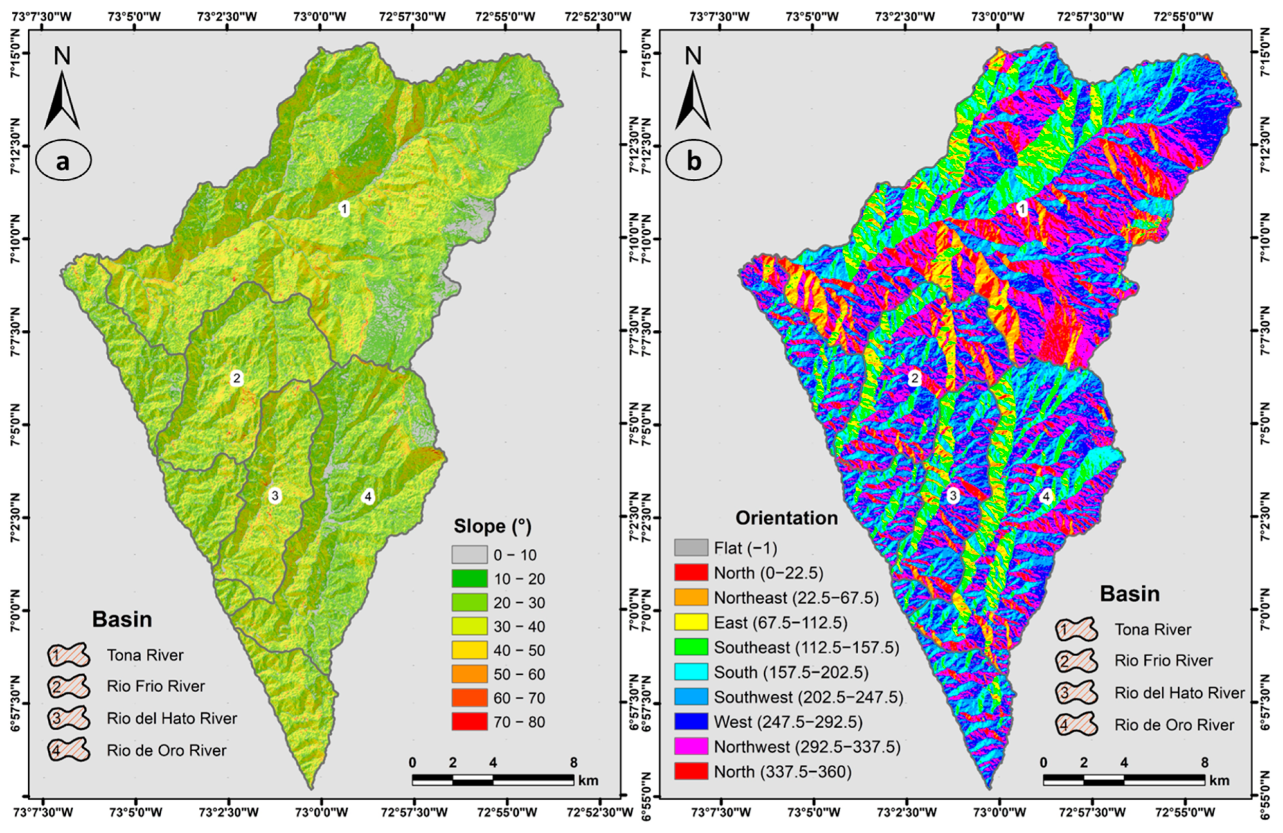
For the slope, the ranges in which mass movements are more affected were classified [
89]. From this, a statistical analysis was generated where the standard deviation of the data is taken as a reference to obtain the classification of the ranges of the slopes. The present statistical classification divided the slope into 8 classes, each one, with a range of 10° (
Table 1). Although it is observed that the slope for the study area has a wide range (min.: 0° and max.: 74.8°), when evaluated with mass movements, the largest amount of area in which the unstable zones occur is between 30° and 40° (39.05% of the MM area). These areas are described as being steep to very steep slopes where there are entrenched processes of the denudational type, with a high possibility of the development of erosive processes where chaotic granular deposits of little thickness can be generated [
90].
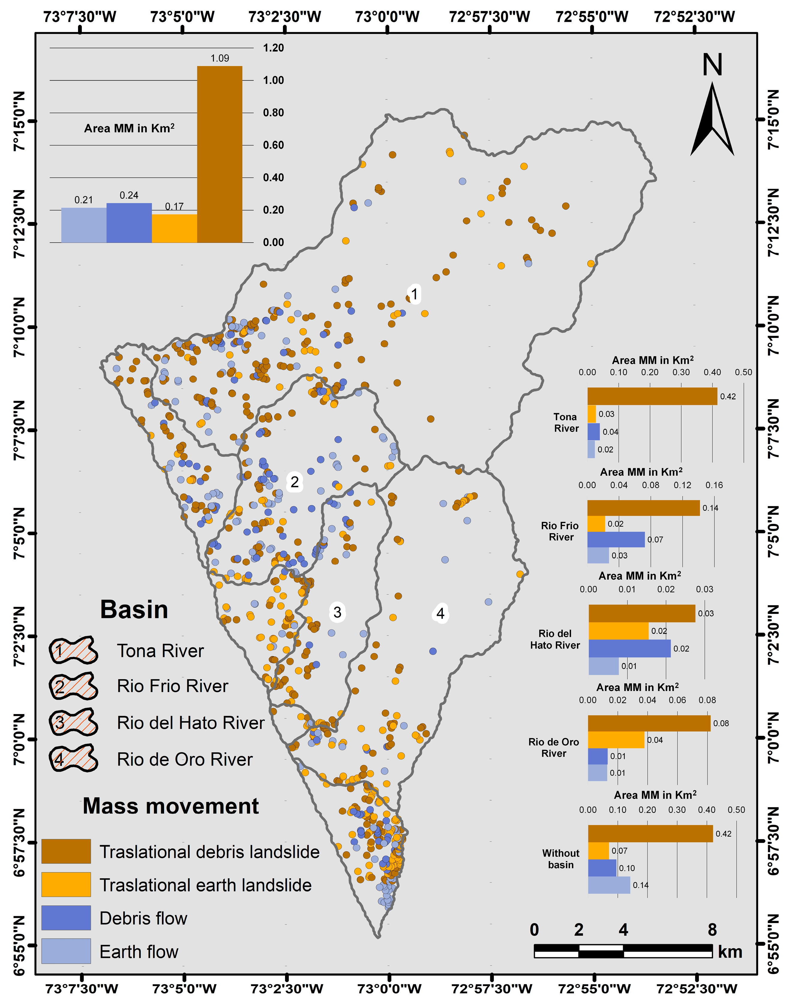
For the rugosity in the study area, it is described that surfaces with a high rugosity present the greatest amount of mass movements (40% of the MM area), followed by surfaces with a medium rugosity (38% of the MM area), a condition consistent with what was described above. For the morphodynamic variable (MM inventory) of the study area, a total of 856 MMs were mapped, with a total area of 1.72 km
2 representing 0.4% of the total area of the region (max. area: 49,903.4 m
2; min. area: 33.5 m
2 affected by an event), with a frequency of 2 movements per km
2 (
Figure 5). These movements are described as, traslational debris landslide with 379 events (1.09 km
2, 63.3%), traslational earth landslide with 205 events (0.17 km
2, 10.1%), debris flow with 113 events (0.24 km
2, 14.1%), and earth flow with 159 events (0.21 km
2, 12.5%). It is also described that 364 events (0.39 km
2, 22.6%) are of surface type and 492 events (1.33 km
2, 77.4%) are of deep type (>2 m thick). Performing an analysis of the basins, it is observed that the Tona River basin presents the largest number of events (323 MM, 0.51 km
2), followed by the Rio Frio basin with 150 MMs (0.26 km
2), Río de Oro basin with 95 MMs (0.15 km
2), and Río del Hato basin with 78 MMs (0.07 km
2); furthermore, the zones that do not have a representation of a hydrographic basin (W/B) present a total of 210 MMs (0.73 km
2), being the zones that present the greatest extension of mass movements over the entire study area. With the present inventory, a selection of MMs is made for the calculation of susceptibility (test) and its subsequent validation. This condition is established in order not to generate trends or biases within the results obtained and are applied for each method. To this end, 50% MMs are selected for test and 50% for validation following the following premises:
Selection of MM randomly;
Randomly selected MMs should have equivalent areas in both test and validation;
The MMs must be spatially distributed;
Within 50% of each selection, you must have 25% of each type of MM described (4 types of MM).
Figure 5.
Spatial distribution of mass movements presents in the study area.
Figure 5.
Spatial distribution of mass movements presents in the study area.
On the other hand, for these MMs, there is a correlation between them with respect to the detonating source since, from the geometric construction and its characterization, a clear pattern associated with the rainfalls is distinguished, where 693 MMs (81%) of these detonating sources could be established. The other 163 MMs (19%) are reported in databases, but do not have a specific description or the condition of the triggering factor associated with the event. From this condition and added to the characteristic of the speeds of displacement of the different types of movements described by Cruden and Varnes [
91], the mass movements such as landslides and flows are grouped for the calculation of the susceptibility of each model.
For the variable of land cover that was acquired from IDEAM for the year 2018, it is taken as a direct variable for the calculation of susceptibility due to the way it was built. The following three aspects were considered for its use: 1. The coverage described for the year 2018 has not undergone considerable changes due to anthropogenic factors in the last decade. 2. The input is sufficiently detailed for the susceptibility calculation. 3. The extension of each of the generated coverages does not simplify the susceptibility function for mass movements. With these aspects, we have a layer with 26 covers where the coverage in high secondary vegetation presents the largest extension affected by mass movements (0.38 km2, 22.06%), followed by the mosaic coverage of crops, pastures, and natural spaces with an extension 0.27 km2 (15.54%) and the high-density forest of the mainland with an extension of 0.25 km2 (14.6%).
The temporal variable describes the behavior of change generated between the years 1990 and 2019 (29 years) for areas where tree cover predominates with a minimum canopy density of 30% and a minimum canopy height in situ of 5 m, with a minimum area of 0.01 km
2 (forest layer). The areas with coverage other than natural forest are called non-forest areas (non-forest layer) [
92]. With the forest–non-forest layers for each year, a cross is made between them, and by means of a relationship in a combination matrix, the classes of persistence, gain, and request of the cover are determined. This relationship allows us to identify the influence of the time variable as a function of mass movements for a period of 29 years. From this relationship it is observed that the greatest amount of mass movements are found in areas that present a persistence of the type of cover (forest and/or non-forest) with an area of 1.34 km
2 (78%), followed by areas with a loss of cover (forest to non-forest) with an area of 0.35 km
2 (20.3%) and, finally, areas that present a gain in the type of cover (not forest to forest) with an area of 0.03 km
2 (1.7%). From this analysis, it would be expected that the areas with a loss of cover would have the greatest amount of mass movements, but this condition generated over areas of persistence may be associated with intrinsic factors of the terrain other than the type of coverage. These factors can be related to the inclination of the land, the type of rock present, the supersaturation of the ground by infiltration, or the structural control that can exert a fragile behavior, giving rise to a degradation of the rock massif by the geomechanical aspects of the rocks. Another important aspect to consider is the variation of forest–non-forest in a period of 29 years, where there is a loss of approximately 60.4 km
2 (2.08 km
2/year). With this rate of change and without variations, an extrapolation is made based on the year 1990 to which it is projected with a loss of 50%. This scenario would be generated by the year 2052 and with a loss of 100% by the year 2112. Based on this analysis, the conditions of instability of the terrain can be extrapolated to the future since the regions described as lost present 20.3% of the area in mass movements, a condition that can increase in a critical way.
4.2. Calculation of Susceptibility
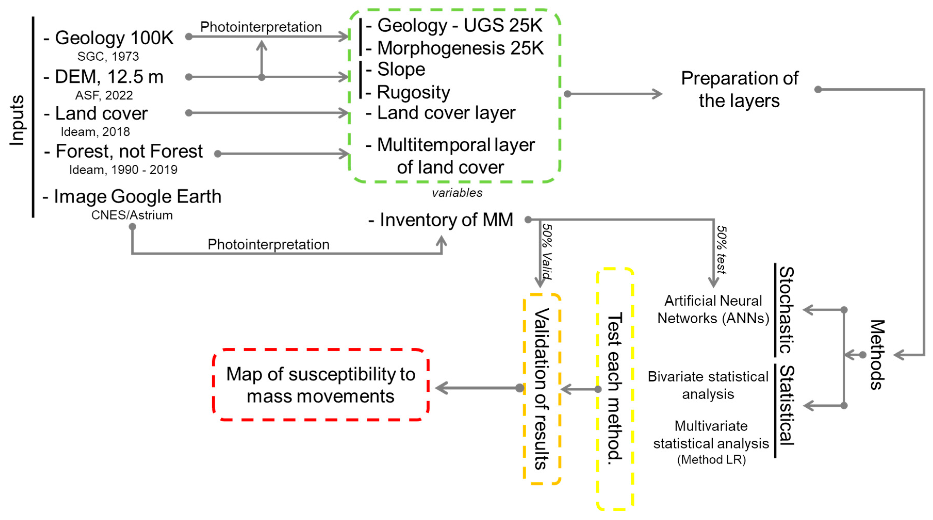
From the geoenvironmental characterization carried out, the calculation of susceptibility by mass movements is generated considering the conditions described in
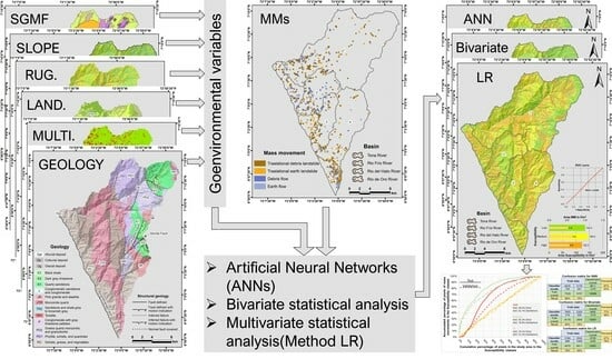
Section 3 and following the methodological scheme proposed (
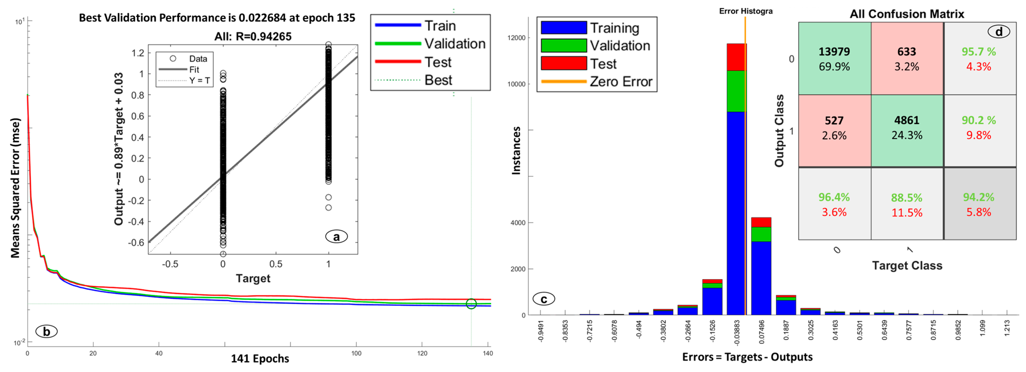
Figure 4). The first susceptibility model was performed by means of the stochastic method under the algorithm of ANN in function BP. For the analysis of the ANN model, a total of 20 architectures were built, where, for each of these architectures, the parameters of the modeling percentage, test percentage, validation percentage, number of neurons, and the type of training algorithm were modified. This is in order to estimate by way of training and its performance in the degree of prediction is measured by the result of the quadratic regression, performance curve, training status, and confusion matrix, thus defining the best architecture in the susceptibility model. As part of the processing to obtain a better performance, the variables were normalized to guarantee a correct correlation between them and the points where mass movements are presented [
71]. Of the 20 architectures, the 6-50-1 architecture (6 variables, 50 neurons, and 1 output) was taken, which has a configuration of 75% data for training, 15% data for validation, and 10% data for testing, in a Levenberg–Marquardt learning algorithm. An important aspect to mention is that, in all simulations, in their training, a standard arrangement was left in the number of iterations (1000), a goal equal to zero (0), and a maximum of failures of 25, in turn, the values taken for training, validation, and testing were distributed internally by the program in 50% of the data of the variables and MMs. These percentages are part of the training form of the algorithm, thus generating a second selection of data, which guarantees a greater degree of confidence when reviewing the goodness of fit of the model [
71]. This selection of percentages can be generated manually (expert criteria) or by the predefined configuration of the program. For the present study, it was decided to leave the values predefined by the program since the data entered in the simulation only represent 50%, and making a decrease in the data in the training does not guarantee an ideal model. The 6-50-1 architecture was taken due to its performance in each of the results, which present quadratic regression values equal to 0.94265 and an overall accuracy of 94.2% within the simulation, added to its performance in training and performance, conditions that in the other architectures describe considerable variations (
Figure 6).
The result of the simulation of the 6-50-1 architecture under the ANN algorithm is processed by GIS for conversion of a numerical factor (ASCII) to a vector characterization and later for classification by categories. This classification is performed by means of the statistical construction by percentiles described above. From this result, it is obtained that the high category of susceptibility presents an area of 139.41 km
2 (34.52%) of the total study area, and on this area, 501 MMs were grouped, which generate an affected area of 1 km
2 (58.57%). The medium category of susceptibility has an area of 179.06 km
2 (44.34%), groups a total of 309 MMs with an area of 0.63 km
2 (36.14%). Finally, the low category has an area of 85.32 km
2 (21.14%) and groups a total of 46 MMs, and an affected area of 0.09 km
2 (5.29%) (
Figure 7). The final susceptibility model represented by the three categories was validated by the ROC curve with a 0.695, describing an optimal goodness of fit.
For the present model, a close relationship is observed between the variables that entered the simulation and the regions that were categorized into the three susceptibility classes. Although, in a specific way, the variables of the slope and rugosity show a better correlation with the areas that present instability and variables such as coverage and temporal present a moderate to high agreement. On the other hand, the ROC (0.695) is below the standards (0.7 or 70%), but the vector characterization and the number of MMs (50% test) that are presented in the high category give an acceptable goodness of fit, a condition that will be evaluated later with the validation of all models with the other 50% of MMs. With the present result, a description was made regarding hydrographic basins in order to determine the percentage of affectation in each basin. To this end, it is observed that, by limiting the model to the basin, regions such as the Rio Frio basin describe a better relationship between the category and the number of MMs (evaluation in high category), on the contrary, the Tona River basin presents a low prediction in the category of high susceptibility and its relationship with the MMs is moderate (
Table 2). The reason for these changes in the form of prediction will be described in more detail at the end of the three methods of susceptibility assessment to have a more complete picture.
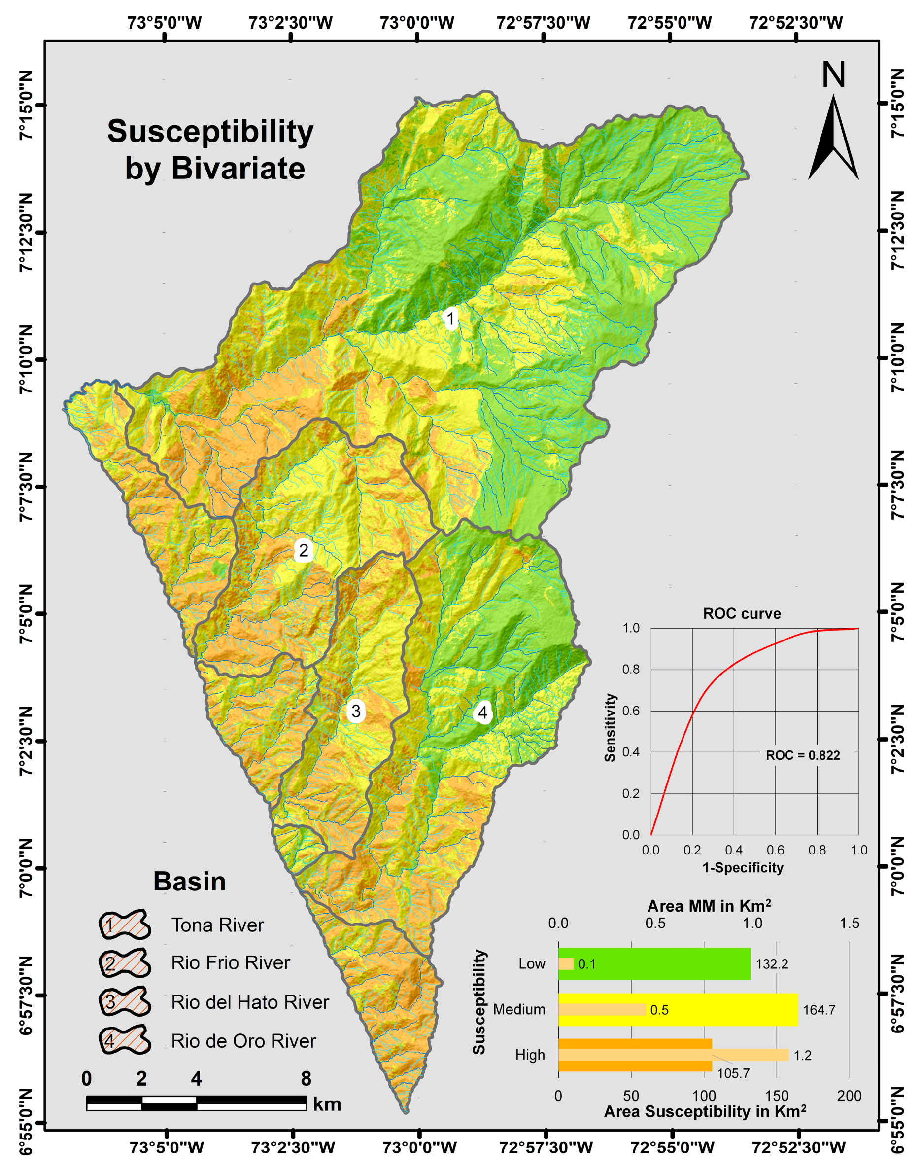
For the susceptibility model generated by means of the statistical method, the calculation of the bivariate statistical analysis is performed first. Due to the form of construction of the present model, it is not possible to establish a relationship in which a variable presents more or less influence on the final result, as described for the ANN, since the bivariate statistical analysis works according to the areas, a weight is established in each attribute within the variable. But you can make a description of the attribute that can give a greater or lesser weight in the variable. As a result, for the present model, it is observed that the high category of susceptibility has an area of 105.65 km
2 (26.25%) of the study area, and on this were grouped 591 MMs with an affected area of 1.19 km
2 (69.21%) of the total area of MMs. The medium category of susceptibility presents an area of 164.65 km
2 (40.91%), groups a total of 225 MMs, with an area of 0.45 km
2 (26.23%). Finally, the low category of susceptibility has an area of 132.16 km
2 (32.83%), groups a total of 40 MMs with an affected area of 0.08 km
2 (4.55%) (
Figure 8).
Within the evaluation of the weights of evidence, it is observed that, the slope variable in the range of 50°–70° contributes to the occurrence of MMs, and the slope between 0° and 20° does not contribute to the occurrence of MMs. An important aspect to highlight in this evaluation is the range of the slope between 50° and 70° since, as mentioned, the present method works on the relationship of the areas and the MMs. Observing this range of the slope, we have a region that presents very little extension, but with a large number of MMs. This is mentioned since in the literature there is a description of a critical range that generates instability on the slopes, which is between 30° and 40° [
93,
94], which is consistent with what is described in
Table 1, but differs from the weight of evidence generated by the bivariate method.
The other contributing variables are (UGS) low-resistance shale rock (PD1) and quartz-monzonite (JTR), (SGMF) very steep erosive slope and pressure loin, (land cover) rocky outcrops and rounds of water bodies of urban areas, (temporary) loss of coverage, and (morphometric) high rugosity. The variables that do not contribute are (UGS) the rock of moderate sandstone resistance (K1) and the glacial transported soil (Qg), (SGMF) the structural slope and the glacio-fluvial cones, (land cover) open shrub and dense grassland with shrubs, (temporary) coverage gain, and (morphometric) low rugosity. From the previous description, it is observed that all the attributes are consistent with the conditions of instability of the surfaces, making an exception of the slope. The final susceptibility model presents a ROC equal to 0.822 that describes a very good goodness of fit. Performing an analysis of the basins, it is observed that the W/B regions describe the best relationship of the category against the number of MMs (evaluation in high category), followed by the Rio Frio basin, on the contrary, the Tona River basin presents a low prediction in the category of high susceptibility and its relationship with the MMs is low (
Table 3).
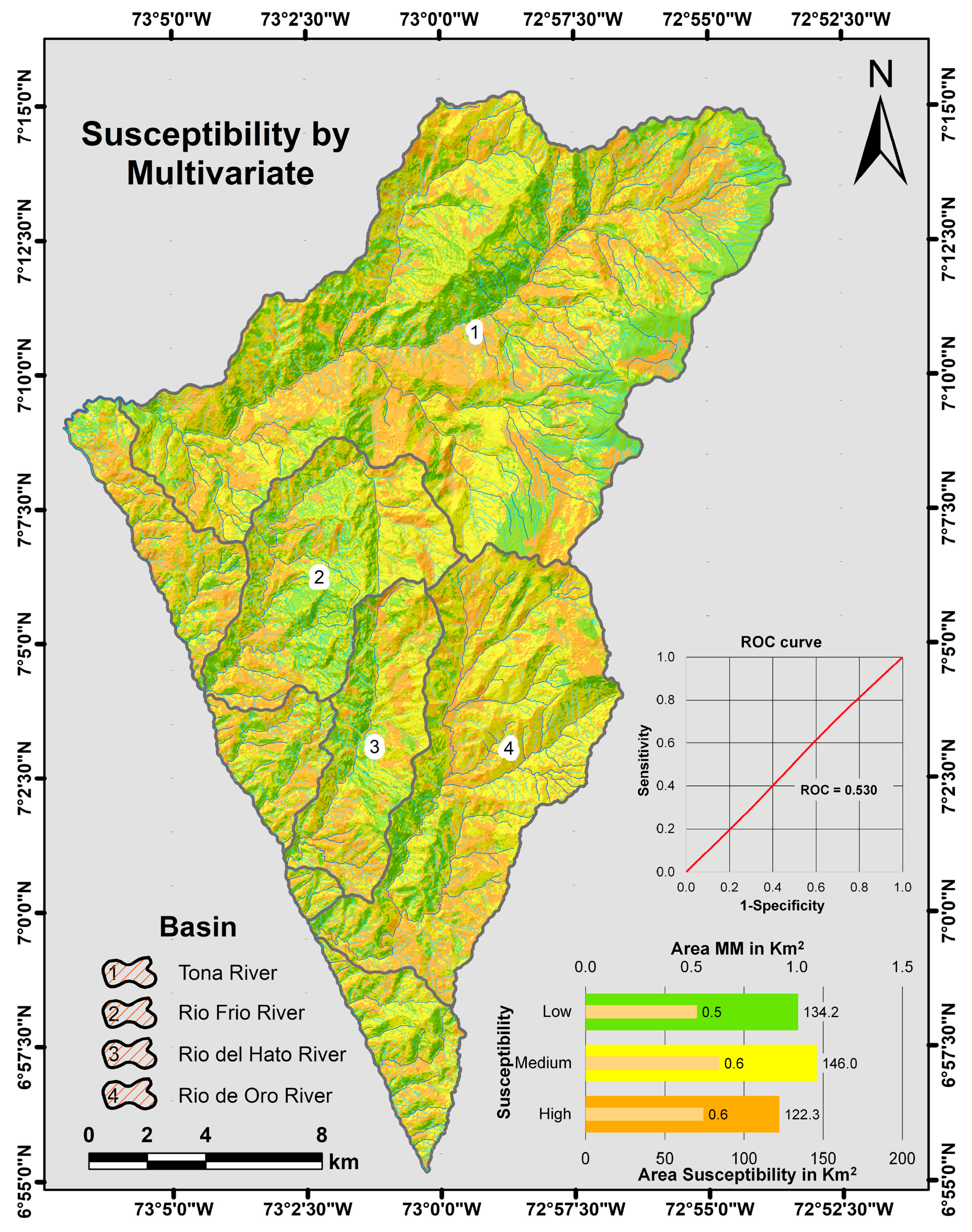
Finally, the susceptibility model is made from the multivariate method created under the LR algorithm. For this model, a total of 16 simulations were generated by modifying the conditions of the dependent and covariate variables, the amount of data entered into the model, and the shape of the data (normalized or in native format). For each simulation performed, the behavior of Cox and Snell’s R
2, Nagelkerke’s R
2, the classification percentage, and the results of the classification table as a function of Wald and Sigmoidal were observed [
81,
82]. Due to the method of classification of the dependent and covariate variables, which does not comply with the assumption of normality in the distribution of the values, a nonparametric test was performed to observe the degree of correlation that extends between the data. For this analysis, the data were evaluated by means of the Spearman correlation to measure the relationship between the two groups from the arrangement generated for each of the 16 simulations (
Table 4).
With each arrangement and its simulation, the one that obtained the best performance in the degree of prediction was evaluated and taken, being the arrangement that presents 5 unnormalized variables, 3 of ordinal type (UGS, land cover, and temporary coverage), and 2 of scalar type (slope and rugosity), with values of Cox and Snell R
2 equal to 0.240 and the Nagelkerke R
2 equal to 0.321, a classification percentage of 69.4%, Wald values greater than zero and sigmoidal without the presence of values greater than 0.5, and data obtained after the last correlation generated. This simulation, in its first Spearman correlation test, showed that the SGMF variable did not present a good correlation since it obtained a result of 0.03 below the standard (0.05), so it was not taken for the final simulation. From the result of the present model, it is obtained that the high category of susceptibility presents an area of 122.3 km
2 (30.37%) of the total study area, and on this area, 257 MMs were grouped with an affected area of 0.50 km
2 (29%) of the total area of MMs. The medium category of susceptibility presents an area of 146 km
2 (36.28%), groups a total of 325 MMs with an area of 0.69 km
2 (40.32%) of the total area of MMs. Finally, the low category has an area of 134.2 km
2 (33.34%), groups a total of 274 MMs with an affected area of 0.53 km
2 (30.68%) of the total area of MMs (
Figure 9). The final susceptibility model has a ROC equal to 0.530, which describes a good goodness of fit. With the present susceptibility model, an analysis is carried out by hydrographic basins, from which it is observed that regions such as the Tona and Río de Oro rivers basins describe the best relationship of the category against the number of MMs (evaluation in high category), on the contrary, the Río Frio basin presents a low prediction in the category of high susceptibility and its relationship with the MMs is low (
Table 5).
With the results generated in each of the models proposed for the calculation of susceptibility by mass movements over the study area, considerable contrasts are observed in the prediction of spatial form. Based on the fact that the calculation is given by the interaction of the variables or inherent conditions of the area with the points where ground movements have been generated, in order to extrapolate these scenarios to regions where no events have occurred but that may eventually be unstable in the future [
71,
94]. These models describe different ways of relating these two conditions, as mentioned above, but their result at the level of spatial analysis determines those sectors that are susceptible to changes, but at a level of procedural control, such as vector construction, they differ from each other. The final models of each method were subjected to their own tests given for each algorithm and the program executed, thus ensuring the selection of the simulation that best represents the relationship between the conditioning factors and the dependent variable; however, each of the final models was given three tests to contract the effectiveness in predicting the data. These three tests are part of the validation in which 50% of the mass movements that were not entered in the initial calculation (creation of susceptibility model for each proposed method) are taken as a basis. These movements were selected according to the specifications described above. The purpose of the present validation was to observe if the model really predicts on the regions that were not entered in the execution of the algorithm. The first validation test was based on the ROC curve and its AUC. The second test was based on comparing the agreement observed between each set of data obtained between the test and the validation of each model, for this comparison the statistical measure of Cohen’s kappa coefficient was taken. The third test consisted of the degree of classification generated from a confusion matrix, and from this, the values of accuracy, precision, recall, and harmonic mean (F1-score) were obtained. For the construction of the confusion matrix, 100% MM (856 MMs) was taken, which was contrasted against the classification of susceptibility represented in three categories for each model. For this process, MM data and susceptibility categories are taken by areas represented in pixels (
Figure 10).
For the susceptibility model created under the ANN algorithm, AUC = 69.5% (test) and AUC = 61.7% (validation), Kappa index (0.592—moderate), accuracy = 63.86%, precision = 0.67, recall = 0.89, and F1-score = 0.76 are described. In the model created under the bivariate algorithm, values of AUC = 82.2% (test) and AUC = 76.9% (validation), Kappa index (0.718—good), accuracy = 73.76%, precision = 0.77, recall = 0.93, and F1-score = 0.84 are described, and for the model generated by the RL algorithm values of AUC = 53.1% (test) and AUC = 51.1% (validation), Kappa index (0.951—very good), accuracy = 59.68%, precision = 0.47, recall = 0.78, and F1-score = 0.58 are described. With the construction of the AUC curves for each method, the Kappa index and the analysis from the confusion matrix and its results, it is observed that the calculation of susceptibility through a bivariate statistical analysis presents a good performance in the prediction both at the level of the calculation by each algorithm, and in the unstable regions that did not enter the model. An important aspect to highlight is that all simulations were performed with 50% of the MMs, which shows that the results present here have a high predictive power independent of the method executed. On the other hand, it is clear to mention that, although the ANN generates an estimate more consistent with this type of prediction models, the correlation of data by means of the bivariate method with weights of evidence simulated the points not entered into the model (test) in a better way. This condition may be associated with the cartographic construction of the variables, which, although these are according to the scale of study, the quantity and differentiation can generate non-optimal trends for the ANN and LR methods.
Once the result of each model from the vector construction was seen, the calculation performed by the bivariate method preserves the spatial relationship of both the mapped events and the areas that have a low susceptibility to mass movements since these regions have surfaces that have a slope <10° and UGS of the hard rocks type little weathered. In general, from the considerations described above, a prediction and quality of the model can be established regardless of the method used, with only 50% of the MM inventoried, but with the clarification that the variables that are really affecting the study area and their correct categorization must be adequately defined.


