Abstract
The water conservation service of an ecosystem reflects the sustainability of regional water resources and is significant to human survival and sustainable development. However, global climate warming and intensified human activities pose substantial challenges to regional water conservation services, especially in an alpine region with a fragile ecological environment, which is more sensitive to climate factors and land use pattern changes. In this study, the Qilian Mountains (QLM) region was chosen as the study area to investigate water conservation trends and drivers in an alpine region. The InVEST model was used to estimate water conservation in the QLM from 2000 to 2020. In addition, the characteristics of the spatiotemporal variation in the water conservation were analyzed using a combination of the Theil–Sen median trend and Mann–Kendall method, coefficient of variation, and Hurst exponent, and the main driving factors affecting these changes were determined using partial correlation analysis and contribution analysis. The main conclusions are as follows: (1) The predicted water conservation in the QLM based on the InVEST model’s water yield module had a relative inaccuracy of 5.96%, and the mean water conservation in the QLM from 2000 to 2020 was approximately 78.08 × 10⁸ m3. (2) The water conservation showed a slight increase over the whole QLM region, with a change rate of 0.565 mm/a; yet, it showed a distinct spatial distribution pattern characterized by “more in the east than in the west”. (3) The contribution of the various land use categories to the total water conservation, from highest to lowest, was according to the following: grassland (62.44%) > unutilized land (15.99%) > forest (11.44%) > cultivated land (9.86%) > construction land (0.45%) > water (0.03%). (4) Precipitation exhibited a significant positive correlation, with contribution ratios of approximately 58.50% to the variation in the water content, whereas potential evapotranspiration and surface temperature showed a nonsignificant negative correlation with contribution ratios of approximately 2.17% and 2.08%, respectively. The results can provide scientific reference for ecological protection in the QLM and other similar alpine environment areas.
1. Introduction
As a cornerstone of life and human well-being, water resources play a significant role in facilitating industrial and agricultural development [1]. They are intricately regulated within ecosystems through a spectrum of hydrological processes encompassing rainfall retention, soil water storage, and freshwater provisioning collectively known as the water conservation service function [2]. The magnitude of water conservation not only mirrors the long-term sustainability of ecosystem water resources but underscores that any imbalance between water production and consumption can severely disrupt the permanent water equilibrium of ecosystems [3]. However, the relentless growth of the global population and the intensification of food production activities significantly heighten the risk of surface and groundwater shortages [4]. This incessant surge in demand renders water scarcity a looming threat to the sustainable development of human society, affecting both temporal and spatial scales [5,6,7]. In response to these formidable challenges, it becomes imperative to undertake rigorous scientific assessments of ecosystems’ water conservation service functions and yield reliable simulation results. These assessments and simulations serve as indispensable tools for policymakers, enabling them to make ecologically informed decisions, improve environmental conditions, and ascertain the status of local water resources, as well as effectively address mounting pressures on local water conservation initiatives [8]. By adopting such measures, we can make substantial contributions to the sustainable development of ecosystems [9,10].
In recent years, significant advancements in GIS technology and the growing focus on ecosystem services research have enabled the quantitative evaluation of water conservation functions and the analysis of their driving factors at the watershed scale [11,12]. Numerous scholars have employed hydrological models to finely and quantitatively simulate and evaluate the water conservation service function of ecosystems in their respective study areas. Several models, including the InVEST model developed by the Stanford Environmental Institute [8,11], the Penn State Integrated Hydrologic Model (PIHM) [13], the Soil and Water Distributed Integrated Model (SWIM) [14], the MIKE System Hydrological European distribution model [15], and the Water Supply Stress Index model (WaSSI) [16] have demonstrated excellent performance across various geographical conditions. The current evaluation of the water-conserving ecosystem service function primarily relies on the water vapor balance method or rainfall storage method [17]. The InVEST model is based on the notion of moisture–heat coupling, which is especially well suited for quantifying the water conservation capability of various spatial cover regions in large-scale watersheds [18]. It facilitates the direct analysis of priority conservation areas at the landscape level and serves as an effective and cost-efficient decision support tool [19]. The Budko theory underpins the InVEST model, which serves as a powerful framework for water volume simulation and testing [20]. The model employs meta-scale calculations, and the output is presented in a visualized form that directly relates to ecosystem services [21,22].
Based on the water conservation data simulated in hydrological models, numerous scholars have endeavored to investigate the spatiotemporal variation characteristics of water conservation in diverse watersheds worldwide. Matios et al. found that water conservation in California’s Central Valley increased significantly through a linear trend analysis year by year [23]. Yohannes et al. found that water conservation in the Blue Nile basin showed a trend of substantial increase based on the ESCI Index method [24], while Aneseyee et al., employing the segmented estimation method, demonstrated a marked decrease in water conservation over the years in the nearby Winike Basin, which is close to the same latitude [21]. Meanwhile, widely used trend analysis methods, such as the EOF, regression, and Mann–Kendall test, were also used by Wu et al. and Eingrüber et al. to analyze trends in water conservation of the Weihe River and western Germany. According to the findings, the Weihe River basin’s water conservation service function has been marginally enhanced, and the water conservation in the upper reaches of the Rur watershed has greatly increased [25,26]. Furthermore, many studies have been dedicated to exploring the key drivers of change in water conservation within watersheds. Bai and Aneseyee et al. summarized that climate warming accelerated the hydrological cycle and was the dominant factor driving the shift in water conservation via comprehensive effects and scenario simulation [10,21]. However, based on the correlation and sensitivity analysis results, Hoyer and Li et al. found that climate change and variations in land use patterns jointly affect the water conservation function of ecosystems [12,27]. In the context of specific wetlands and forest zones, Hu’s research, which is rooted in principal component analysis and cluster analysis, underscored that the impact of land cover changes on water conservation significantly surpasses that of climatic variables [17]. However, the existing land cover datasets do not fully consider the characteristics of QLM and do not possess long temporal coverage, high resolution, and high accuracy all at the same time. For example, Chen et al. successfully developed a 30 m land cover data product, GlobeLand30, with an accuracy of 83.5%; however, it only included three phases: 2000, 2010, and 2020 [28]. Consequently, a long-term land cover classification dataset was developed in this study, with a resolution of 30 m and an accuracy of 82.5%, encompassing a time span from 2000 to 2020. In general, most studies concerning the trends and attributions of water conservation have been conducted in small watersheds, primarily located in tropical and subtropical regions. However, studies in high and cold regions remain limited. Considering the fragile ecological environment and heightened sensitivity to climate and land use factors in alpine regions, trends in water conservation and their underlying mechanisms exhibit distinct spatiotemporal variation characteristics compared to other areas. In addition, land use datasets applied to large-scale areas often cannot meet the requirements of resolution, accuracy, and long-term continuity of data at the same time. In addition, existing attribution analysis studies primarily concentrate on qualitatively assessing the relationship between water conservation and its driving factors, lacking quantitative analysis.
To mend these critical gaps, this study selected the Qilian Mountains as the study region and utilized the InVEST model to estimate multiyear water conservation. Based on the simulated water conservation results, the evaluation methods of the Theil–Sen median trend and Mann–Kendall method, coefficient of variation, and Hurst Index were integrated. The spatial and temporal evolution of water conservation in the Qilian Mountains were evaluated more clearly and systematically from the characteristics of the interannual variation and fluctuation in the time scale and the pattern distribution and dynamic trend in the space scale. In contrast to earlier studies, which preferred the use of scenario simulations or a single correlation analysis to qualitatively assess how sensitive water conservation is to driving factors, we also conducted a quantitative contribution analysis on the impact of various driving factors on the change in water conservation on the basis of partial correlation analysis. The key variables influencing the basin’s water conservation service function were further identified. The overarching goal of this research was to systematically elucidate the impact of climatic conditions and land cover types on regional water conservation at a certain stage within a coherent theoretical framework. A variety of methods were used to determine the specific impacts of each driver and to establish a vital linkage between available freshwater resources in mountainous areas and the water requirements of neighboring residential communities. This linkage holds promise for alleviating seasonal and regional water scarcity while enhancing our comprehension of potential hydrological mechanisms [29], thus contributing to the judicious allocation of water resources.
2. Materials
2.1. Study Area
Located in the border area between Gansu and Qinghai provinces in northwest China, the Qilian Mountains (QLM) (35°50′12″–39°58′15″N, 93°33′27″–103°53′43″E) are renowned as the “Mother Mountains of the Hexi Corridor” because of their crucial role as a barrier safeguarding the ecological security of the three rivers. The QLM extend over a vast area with a wide range of topography and large undulations [30]. The mountains in the study area are widely distributed from southeast to northwest [31], with elevations ranging from 4000 to 5500 m. There are 10 major cities in the study area, including Baiyin, Jinchang, Jiuquan, Lanzhou, Wuwei, and Zhangye, Haibei Tibetan Autonomous Prefecture (Haibei), as well as Haidong, Hainan Tibetan Autonomous Prefecture (Hainan), Haixi Mongolian Tibetan Autonomous Prefecture (Haixi), and Xining, see Figure 1. The QLM are positioned far from the coast, at the confluence of three plateaus, namely, the Qinghai–Tibet Plateau, Mongolian Plateau, and Loess Plateau, having a characteristic alpine cold and subhumid mountain climate [32]. The annual precipitation ranges from 300 to 700 mm, primarily distributed by topographic rain [33]; the average annual evapotranspiration exceeds 1000 mm, while the annual surface temperature is approximately −15–35 °C. Permafrost is widespread throughout the QLM, while the glacier over the QLM accounts for approximately 3.7% of the total glacier area in China. The temperature and precipitation vary with altitude, resulting in distinct vertical vegetation zones from low to high altitudes [31]. The predominant plant type in the QLM is grassland, which accounts for around 40% of the total area. As such, the QLM serve as a significant animal husbandry production base and a vital ecological protection forest belt supporting wildlife migration corridors in western China [34,35]. From 2000 to 2020, the natural environment of the QLM has shown a tendency towards ecological fragility due to global warming and anthropogenic activity. The decline in vegetation cover poses challenges to the sustainable development of water conservation services and local water resources management.
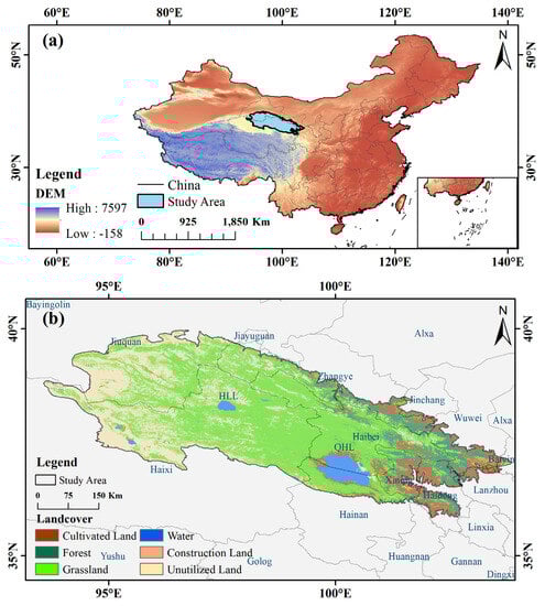
Figure 1.
The location of the Qilian Mountain Watershed: (a) geographical location and digital elevation model of the study area in China; (b) spatial distribution of land use types, administrative boundary of the study area, and the two main lakes—Hala Lake (HLL) and Qinghai Lake (QHL).
2.2. Data Sources
Several datasets were employed to simulate and predict the study area’s long-term water conservation, including land use, annual average precipitation, annual average potential evapotranspiration, plant available water content, root depth, DEM, watershed division map, topographic index, velocity coefficient, parameter Z, and GLEAM land evaporation. In addition, the influence of climatic conditions and land use patterns on water conservation was investigated by considering land use, annual average precipitation, annual average potential evapotranspiration, and annual average surface temperature. Land use types were categorized as cultivated land, forest land, grassland, water bodies, construction land, and unutilized land. In this study, several data preprocessing steps were undertaken to ensure data consistency. Firstly, we standardized the data coordinates by projecting all data into the Krasovsky_1940_Albers coordinate system. Subsequently, we refined the research area by cropping their scope, resulting in a more focused dataset. To enhance the data resolution, all raster data were resampled at a uniform 1000 m scale using nearest neighbor resampling. Moreover, monthly data were aggregated on an annual basis, preserving the dataset’s temporal continuity for the period spanning 2000 to 2020. In previous studies, the meteorological data [36,37,38,39], DEM data [40], and soil data [12,17] used in this study were all verified for accuracy and universality. Table 1 represents further information regarding the data as follows:

Table 1.
The details of the data used in this study.
3. Methods
The purpose of this study was to examine the spatiotemporal changes in water conservation service function in the alpine region and quantitative analysis of the influence caused by the driving factors. In this study, a regional land use dataset over QLM was created using Landsat remote sensing data and various machine learning models. Combined with precipitation, potential evapotranspiration, plant available water, root depth, and other parameters, multiyear water yield was estimated using the InVEST model. Based on this, the Z coefficient of the model was adjusted by comparing the GLEAM evapotranspiration product set with the actual evapotranspiration output to reduce the relative error. According to the water balancing principle, the surface runoff was adjusted by taking the regional land topographic index, velocity coefficient, and information on the conductivity of the saturated water in the soil into account, and the QLM regional water conservation dataset from 2000 to 2020 was generated.
The Theil–Sen median trend and Mann–Kendall method (Sen + MK), unitary linear regression, coefficient of variation, and HURST Index methods were utilized to analyze the interannual variation and fluctuation characteristics, spatial pattern, and dynamic trend of the water conservation service function over the QLM from 2000 to 2020 on the basis of the precision evaluation and visualization of the dataset. Multivariate evaluation techniques of land class analysis, partial correlation analysis, and contribution degree analysis were used to quantitatively analyze the impacts of various land use types and meteorological factors (precipitation, potential evapotranspiration, and surface temperature) on regional water conservation. Realistic recommendations were obtained using the temporal and geographical fluctuations in the water conservation service function and the quantitative effect of the driving forces. Figure 2 provides an overall framework flowchart illustrating the methodology employed in this study.
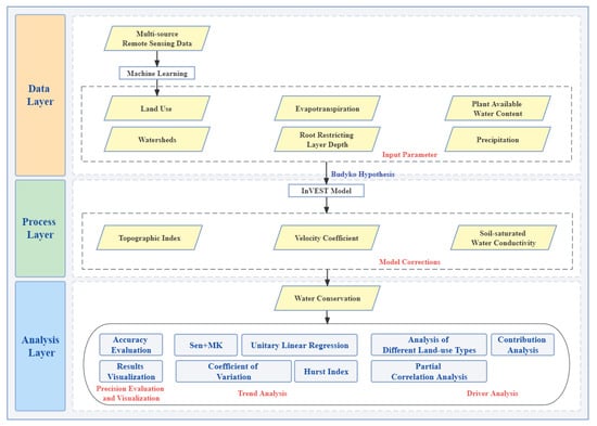
Figure 2.
Overall research framework.
3.1. Land Classification
At the regional scale, land use/land cover (LULC) exert a considerable influence on habitat quality. Variations in land use/cover cause variations in the surface albedo, local water vapor cycling, and surface circulation, consequently, affecting regional climate patterns and introducing discrepancies in water conservation estimations. The total area of the permafrost in the QLM is approximately 8.03 × 10⁴ km2, accounting for about 47.51% of the region [50]. Considering escalating impacts of climate warming, the permafrost undergoes extensive degradation, resulting in increased active layer thickness (ALT) and the melting of underground ice. Changes in surface water conditions triggered by variations in ALT significantly impact production, convergence processes, and ecological dynamics within the permafrost zone [9]. Furthermore, with the growth in the number of Qinghai–Tibet projects, human activities have a significant influence on the assessment of LULC, particularly in the context of Qinghai–Tibet projects. These activities have the potential to modify surface albedo, local water vapor cycling, surface circulation, and other objective factors, thereby affecting regional climate patterns and introducing deviations in water content estimations.
Therefore, this paper selected the thawing index and nightlight as predictors to represent the extent of permafrost degradation and the intensity of human activities, respectively. In addition, spectral features (bands: red, green, blue, NIR, SWIR1, and SWIR2) and ten remote sensing indices obtained from Landsat images, including NDVI, NDWI, etc., along with topography were selected as predictors. All these aforementioned parameters were combined to make feature collections. Additionally, the labels were selected from the geometric center of the long-term stable and unchanged regions of the GlobeLand30 temporal datasets. Of all of the labels, 70% was randomly collected for the model’s training, and the other 30% was utilized for the accuracy’s validation. Different machine learning models were established and estimated, and the optimal one was selected for mapping the temporal land classification dataset based on the accuracy of the evaluations. Figure 3 provides a flowchart of the construction of the temporal land classification datasets.
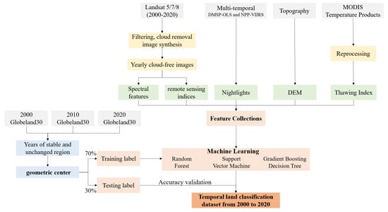
Figure 3.
Flowchart of the construction of temporal land classification datasets.
3.2. Water Yield
The InVEST model, established together by Stanford University, the Nature Conservancy, and other organizations, including the Integrated Valuation of Ecosystem Services, is a natural service evaluation model that allows for the modeling of ecological service evaluations under diverse land use scenarios. The InVEST model fosters informs decision making by providing scientific insight and understanding of the consequences of human actions to decision-makers [34]. Based on the Budyko theoretical structure, the “Water Yield” module of the InVEST model establishes relationships between the water yield and factors including precipitation and energy, as well as potential evapotranspiration. This module has great promise for investigating and measuring the effects of the changing climate on ecological water conversation services [51].
The basin’s water yield was obtained through the calculation of precipitation, root-limiting layer depth, and potential evapotranspiration, as well as the available water content of plants. Among these, precipitation can be divided into evapotranspiration and runoff processes, and the runoff procedure is attribute to the difference between atmospheric water vapor demand and water supply [52]. The formula of the InVEST model’s water yield module is as follows:
where represents the water yield in the type j LU mode of grid x; denotes the actual annual evapotranspiration in the type j LU mode of grid x. serves as the annual precipitation of unit x, while the evapotranspiration distribution is an approximation of the Budyko curve. is the Bydyko dryness index [53], which is equal to the potential evapotranspiration divided by the precipitation; represents the nonphysical parameter that modifies the vegetation’s annual water availability and precipitation. is the vegetation evapotranspiration coefficient in the type j LU pattern of grid x. denotes the evapotranspiration towards reference crops. Z stands for the Zhang coefficient, representing the seasonal characteristics of precipitation. In this project, the evapotranspiration simulation results of the GLEAM dataset in the Qilian Mountains research area were used to debug the Zhang coefficient each year. serves as the available water content of plants, which can be estimated using soil composition data, and the formula is as shown below [54]:
where , , , and are the contents (%) of sand, silt, clay, and organic matter, respectively.
3.3. Water Conservation
Based on the parameters, including topographic index and soil saturated hydraulic conductivity, as well as the velocity coefficient, the aforementioned water production results were modified to obtain the regional water conservation:
where Water Conservation serves as the water conservation (mm); Velocity represents the velocity coefficient; TI is the topographic index; Ksat refers to the soil-saturated water conductivity (mm·d−1), which can be calculated according to the soil parameters, including the soil clay, silt, and sand content; Drainage_Area indicates the number of grids in the catchment area; and Soil_Depth stands for the soil depth (mm), while Percent_Slope refers to the percentage of the slope.
3.4. Trend Analysis
A trend analysis involves examining changes under natural states and providing insight into future trends. In this study, various trend analysis methods were employed, including the one-dimensional linear regression method, Theil–Sen median trend and Mann–Kendall method (Sen + MK), coefficient of variation method (CV), and Hurst exponent on the basis of R/S analysis (HURST).
3.4.1. Unitary Linear Regression Model
The change of water conservation was measured using linear regression, and the slope of it represents the change scope. The formula is as follows:
where Slope is the linear regression slope; i refers to the independent variable of year; n is 21 years; and Water_conservationi is the water conservation in year i. If Slope > 0, this denotes that the water conservation experienced an upward trend, while if Slope < 0, this indicates a downward trend.
3.4.2. Theil–Sen Median Trend and Mann–Kendall Method
This method effectively mitigates the impact of data outliers and allows for differentiation between natural fluctuations and significant trends in various natural processes. It has been widely used in fields such as ecology and hydrology. The formulas utilized in this method are as follows:
where represents the estimated trend value of the series; and represent the level of water conservation in the years i and j, respectively; S stands for the test statistic, while sgn() refers to the symbolic function; var() is used to calculate the variance; Z represents the test statistic trend; and n is the length of the time series, which was 21 years. n > 10, so statistic S approximately followed the standard normal distribution, and the trend test was performed using statistic Z. At the given significance level of , when , it is considered that there exists a severe change in the sequence, not the opposite.
3.4.3. Coefficient of Variation Method
The coefficient of variation (CV), utilized to investigate the fluctuation features of water conservation, is defined as the division of the standard deviation (SD) to the mean value. The formula for its computation is as follows:
where C serves as the CV; S represents the SD; and refers to the average value. The smaller the CV of water conservation, the smaller the fluctuation.
3.4.4. Hurst Exponent
The Hurst exponent serves as a significant tool for accurately and consistently forecasting future trends in a variety of time series. In this work, it is evaluated on the basis of the R/S analysis method, while the future trends are examined using the findings of a sustainable analysis of the QLM’s water conservation from 2000 to 2020.
During a time series, the mean sequence for any positive integer is defined as follows:
The cumulative deviation, range, and standard deviation are, respectively:
The Hurst Index is:
where represents the mean series; represents the arbitrary positive integer; , , and stand for deviation, range, and standard deviation, respectively. H represents the Hurst Index. When H = 0.5, this indicates a random time series with no long-term correlation. When 0 < H < 0.5, this represents that, in contrast to a past trend, the change process is anti-continuous. When 0.5 < H < 1, this denotes that the change process is continuous and familiar to a trend in the past. The closer H is to 1, the stronger the persistence.
3.5. Land Use Transfer
The land use transfer matrix (LUTM), as a traditional approach for studying the transfer direction and quantity change of diverse LU patterns, can directly depict the transformation of various land use types. This method captures the quantitative characteristics of area transfers for different land types over the QLM during the period from 2000 to 2020. The results of the LUTM were associated to changes in the water conservation, and the connections were contributed to a better understanding of how land use variables affect ecosystem water conservation services.
3.6. Partial Correlation Analysis of Climate Factors
Partial correlation analysis (PCA) serves as a statistical technique utilized to evaluate the correlation between regional water conservation and individual climate factors while controlling for the influence of other climate factors. It allows for the exploration of the degree of influence of major climate driving factors on the water-conserving function. After calculating the results of the water conservation, PCA was used on the three major climate factors, namely, PRE, PET and LST after preprocessing the data in the QLM using MATLAB. The PCA between the specific climate factors and water conservation was obtained while controlling for the other two factors. Significance tests were also employed to determine the statistical significance of the obtained partial correlation coefficients.
3.7. Contribution Analysis
Quantifying the influence of the various parameters on the overall water conservation is critical for formulating reasonable water resource management plans and anticipating the changing effects of the climate and human behavior on future water conservation. It provides a feasible way for addressing climate change challenges. The Pearson coefficient method is widely utilized to perform a correlation or sensitivity analysis of each driving factor and further obtain the specific contribution degree of each factor. Alternatively, an analysis of variance is used to differentiate the self-error of different conditions to determine the degree or magnitude of their influence. In this study, according to different LU patterns, a spatial statistical method was adopted. The unit water conservation capacity was used as a representative of the water conservation ability of the land use type (LUT) and, consequently, using the whole water conservation of the LUT to investigate its attribute to the water conservation service function of the ecosystem.
This study focused on investigating the effects of each climatic parameter to better comprehend the unique influences of climate factors on the variation of water conservation. In addition to the attribution to specific climate factors, this research extended the long-term changes to trend attribution. The contribution degree of each climate factor to the water-conserving service function was investigated by quantifying the changing trend of water conservation into the differential expression. The relative effects of the components were measured to help understand the significance of the climate parameters in water conservation.
3.7.1. Analyzing the Water Conservation Capacity of Different Land Use Types and Their Contribution to Water Conservation
Based on the principles of water balance, the InVEST water yield module combined with the water conservation model assumes that on the raster cell catchment area, precipitation minus evapotranspiration leaves in the form of runoff. The model does not differentiate between surface runoff and subsurface runoff [55], instead focusing on simulating the ecosystem’s capacity to retain water at a specific spatial and temporal scale, which directly relates to the land use pattern. Variations in water yield among land classes mainly stem from differences in soil moisture, evapotranspiration capacity, deadfall thickness, and canopy interception [56,57].
In this study, the land use types (LUTs) in the QLM were classified into six categories, including cultivated land, forest, grassland, water bodies, construction land, and unutilized land (in which glaciers and snow were included in the unutilized land cover types). The water yield of each LUT indicates its water conservation capacity, while the contribution of the different LUs towards the total regional water conservation over the QLM during the period from 2000 to 2020 was investigated based on the area of each unit of LUT. Furthermore, the study also explored how different LUTs contributed to the overall water resources. Combined with the results of the land-use transfers, the factors driving changes in the water-conserving capacity and the importance of each LUT were explored from the perspective of human activities.
3.7.2. The Effects of Different Climatic Components Based on the Results of the Trend Analysis
Multiple regression models are widely utilized in hydrologic studies to quantify the contribution of different drivers and determine their relative importance [58]. The water balance concept provides a valuable theoretical framework for evaluating the hydrologic response of a watershed, where precipitation (PRE) and energy (PET) are the predominant drivers [59,60]. Additionally, potential evapotranspiration is influenced by other climatic factors such as temperature [61]. Therefore, this study took the specific effects of PRE, PET, and LST on water source conservation into consideration. In order to explore the relationship between variations and changes in the water conservation and climatic conditions, the change in water conservation was described using the following comprehensive differential representation [62]:
Considering the coherence of the long time series dataset, the main influence of the amount of change (i.e., trend) in the climate factors on the amount of change (trend) in water conservation can be quantified using the following equation:
The magnitude of a factor’s influence (contribution) on the trend in water conservation can then be expressed as:
The following three stages were used in this study to evaluate the influence of significant climatic conditions on the water conservation trend:
Firstly, obtain the time-dependent trend of each climate component and amount of water conservation during the period 2000–2020 through a trend analysis;
Secondly, determine the regression coefficient of each climate component on the amount of water conservation utilizing multiple linear regression;
Finally, quantify the impact of each climate factor on the trend of water conservation using the formulae.
By following these approaches, it becomes possible to effectively classify the influence of climate factors at the scale of raster cells.
4. Results
4.1. Land Classification
In this study, we utilized the Google Earth Engine cloud platform to acquire multisource remote sensing data. The long-term stable regions from the Globeland30 dataset were selected as the labels. The land classification dataset was constructed using random forest. The average accuracy of the dataset from 2000 to 2020 was found to be 82.5%, with a kappa coefficient of 0.803 (Figure 4). Table 2 represents the kappa coefficients of each land classification type, with the water bodies exhibiting the highest kappa coefficient, while the unutilized land demonstrated the lowest kappa coefficient.
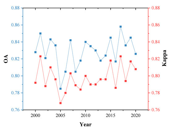
Figure 4.
The accuracy and kappa coefficients of the land classification from 2000 to 2020.
Table 2.
The kappa coefficients of each land classification type.
In this study, the random forest weight analysis method was utilized to investigate the weights of different features (Figure 5). The results reveal that elevation, nightlight, and thawing index exhibited the highest weights, providing evidence that human activities and the process of glacier and permafrost melting, indeed, had a significant impact on land cover during the period from 2000 to 2020.

Figure 5.
Weighting chart of the features utilized in the construction of the land classification.
4.2. Accuracy Evaluation
Evapotranspiration (ET) is an essential component of the water balance and energy balance, making it valuable in water resource change and evaluation and water resources development and management [63]. The ET dataset, based on the water balance equation, can be reliably applied for hydrological applications and validation of water balance components on a multiyear scale [64,65]. Considering data accessibility, this study primarily relies on the GLEAM remotely sensed evapotranspiration data products. By comparing the actual ET data output from the water production module, the Z coefficient was adjusted appropriately to reduce the relative error between the actual ET and GLEAM data to verify the model [63]. Through repeated debugging of the actual evapotranspiration output for each year, the maximum relative error of the total water production in the QLM was no more than 13.814%. The average relative error over multiple years was approximately 5.958%, demonstrating the robustness of the model. The input Z parameters of the model and the corresponding year-by-year errors are represented in Table 3.
Table 3.
Z coefficient and the corresponding error for each year.
4.3. Trend Analysis
The water yield simulation results were modified by combining the water conservation formula to obtain the multiyear water conservation changes in the QLM. The findings indicate that the average unit of water conservation in the QLM over multiple years is 47.52 mm. Furthermore, the total average water conservation in the QLM during the period from 2000 to 2020 amounts to 78.08 × 10⁸ m3.
Based on the interannual variation and fluctuation characteristics observed in the QLM region’s water conservation, the annual unit water conservation trend exhibited a slight upward trend, with a modest change rate of 0.565 mm·a−1 from 2000 to 2020, indicating small interannual variability (Figure 6a). Employing a natural discontinuous approach, the results of the variation and fluctuation analyses were categorized into five groups: low fluctuation (0–0.199), relatively low fluctuation (0.199–0.537), medium fluctuation (0.537–0.900), relatively high fluctuation (0.900–1.621), and high fluctuation (1.621–4.574). These outcomes, as depicted in Figure 6b, reveal that the mean coefficient of variation for water conservation across the entire region stood at 0.455. The medium- and low-fluctuation states collectively accounted for approximately 64.447% of the total region, indicating overall stability in the regional water conservation service function. Furthermore, the results stemming from the Sen + MK trend analysis (Figure 6c) and the future trend prediction results combined with the HURST Index (Figure 6d) suggest a marginal increase in the total water conservation within the study area at present but also potential degradation in the future. The transient rise in the unit water retention observed throughout the entire phase could be attributed to vegetation restoration catalyzed by hydrothermal resources and ecological engineering, collectively enhancing soil and water conservation in the QLM. Conversely, the years marked by abrupt declines may be linked to the reduction in natural land cover due to urbanization and related factors.
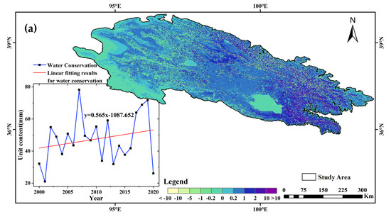
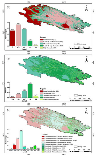
Figure 6.
The temporal trend distribution of changes in water conservation trends from 2000 to 2020 in the QLM region: (a) spatial distribution of water conservation trends depicted using the unitary linear regression model; (b) fluctuation pattern of water conservation assessed with the coefficient of variation method; (c) dynamic change trend of water conservation derived using Theil–Sen median trend and Mann–Kendall method; (d) forthcoming changing trend in water conservation predicted using the Hurst Index method of R/S analysis.
From the results of the analysis of the spatial pattern and dynamic trend, there was a noteworthy regional disparity in the average water conservation over the 2000 to 2020 period, with a discernible upward trend from west to east, as illustrated in Figure 7. The Sen + MK trend analysis results, depicted in Figure 6c, and future trend predictions in conjunction with the Hurst Index, as shown in Figure 6d, collectively indicate an overall upswing in water conservation across the QLM during this period, albeit with some places showing a fragmented reduction. Enhanced water conservation service functions encompass 59.753% of the entire QLM region, as detailed in Table 4. This stage’s dynamic pattern, likewise, indicated an increasing tendency from west to east in space. However, in the forthcoming stage, approximately 50.213% of the QLM area, as noted in Table 5, is projected to witness a reversal in the continuous improvement of water conservation service functions (i.e., degradation). The whole region shows a slight trend of deterioration, with eastern areas witnessing a sustained increase in water conservation, while the western regions are experiencing a marginal decline. As climate factors persistently exert their influence and land use patterns evolve, this trajectory is expected to amplify the differentiation in water conservation service functions across the spatial landscape of the QLM in the future.

Figure 7.
Spatial distribution of the coefficients of the variation in the water conservation from 2000 to 2020 in the QLM region.
Table 4.
Trend statistics.
Table 5.
Statistics on future trends.
4.4. Land Use Transfer
Year-to-year variations in vegetation-cover-induced changes in land use patterns have substantial implications for the ecological and ecosystem service functions of the environment [66]. The analysis of the land use pattern transitions in the QLM during the period from 2000 to 2020, as shown in Figure 8, reveals that in the development stage, construction land was mainly expanded at the expense of cultivated land, forest, grassland, and other ecological land [67]. In the ecological restoration stage, the policy of converting cultivated land to forests was put into execution, effectively increasing the regional coverage, leading to improved soil runoff and water-conserving capacity after more than a decade of vegetation restoration [68].
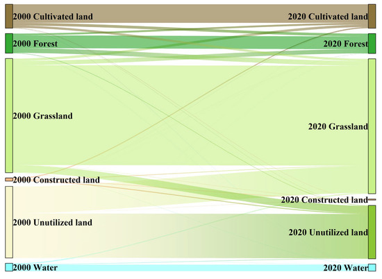
Figure 8.
Multiyear land use transfer results.
The research region’s area of land with outstanding water conservation ability significantly expanded, because a large amount of unutilized land was turned into grassland. These transformations, facilitated by years of deliberate development and timely policy adjustments, have substantially contributed to the environmental ecological restoration in the QLM, bolstering the ecosystem’s water preservation capabilities. Additionally, it was also observed that the water bodies and unutilized land areas showed a decreasing trend, and the glacier retreat and snow melt in the study area may be affected by global warming.
4.5. Partial Correlation Analysis of Climate Factors
Alterations in PRE directly impact runoff, consequently, affecting the spatial and temporal distributions of water resources [69]. On a temporal scale, the variation trend of the unit WC was in compliance with the multiyear trend of the PRE but contrary to the multiyear variation trend of PET (Figure 9). The PCA between water conservation and PRE in the QLM (Figure 10) reveals a significant positive correlation, primarily distributing in 97.813% of the QLM, except some southwest areas of the Haixi Mongolian and Tibetan Autonomous Prefecture. However, the western part of the Haixi Mongolian and Tibetan Autonomous Prefecture, as well as the central part of the Haibei Tibetan Autonomous Prefecture, exhibited a very significant positive correlation with PRE (r > 0.9).
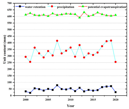
Figure 9.
Annual water conservation, PRE, and PET trends.
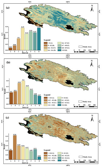
Figure 10.
The results of the bias correlation analysis between WC and climatic factors: (a) partial correlation coefficient map for PRE; (b) partial correlation coefficient map for PET; (c) partial correlation coefficient map for LST.
Evapotranspiration plays a pivotal role in the terrestrial hydrological cycle [70]. PET is defined as the amount or rate of water evaporation from moist soil and from plants and is closely related to actual evapotranspiration [71]. The correlation between the PET factor and water conservation is predominantly negative, covering 58.204% of the QLM, excluding the south of Hala Lake and Wuwei city and Baiyin city. Jiuquan city to the northwest and Haixi Mongolian and Tibetan Autonomous Prefecture to the southwest demonstrated a severe significant negative correlation (r < −0.4) with PET. Furthermore, there exists a mainly negative correlation between the LST factor and WC, accounting for 65.341% of the study areas. While the Haibei Tibetan Autonomous Prefecture and Zhangye city in the east, Jiuquan city in the north (except glacier snow wetlands and other areas without water conservation capacity) showed a significant negative correlation with LST (r < −0.4).
4.6. Contribution Analysis
4.6.1. For Different Land Use Types
The water conservation capacity of various land units in the QLM can be ranked as follows in descending order: forest > grassland > cultivated land > unutilized land > constructed land > water bodies. Within the study area, forest vegetation is mainly dominated by species such as Qinghai spruce, mountain poplar, white birch, and Qilian round Berlin. These species have a large soil porosity, and their canopies and deadwood effectively retain water and slow down runoff. Additionally, the roots of these trees provide stability and contribute to better soil water-conserving capacity. Therefore, the forest exhibits the strongest ability to retain water and contain nutrients. The majority of the grassland in the study region is in the form of alpine meadow, which is a type of nonzonal grassland that developed on the plateau and high mountains, and the soil is intertwined with the root system of the surface layer of the meadow, which is soft, tough, and elastic. This type of soil has a good capacity to support nutrients, contributing to the water conservation ability of the grassland. On the other hand, unutilized land, constructed land, and water bodies exhibited relatively lower water-conserving capacities.
The total quantity of water conserved by various LU categories is listed in the following order: grassland > unutilized land > forest > cultivated land > construction land > water bodies. Grassland, being widely distributed in the study area and possessing remarkable water-conserving capacity, contributes the most to the total water resources. On the other hand, the average water-conserving capacity of unutilized land units is equivalent to that of water bodies, as well as construction land units, but the overall quantity of water conservation is greater because of their larger area.
Based on these findings, the average contribution of different land classes to the regional water conservation in the QLM from 2000 to 2020 was obtained (Table 6). It is evident that grassland plays a predominant role in the region’s water resources, accounting for approximately 60%. Following grassland, unutilized land and forested areas contribute about 15% and 10%, respectively, to the total water conservation (Figure 11). Accordingly, it is estimated that in the near future, the study area will continue to rely on grassland for approximately 60% of the total water amount, while unutilized land and forested land will contribute approximately 15% and 10%, respectively.
Table 6.
Contribution of the different land use types.
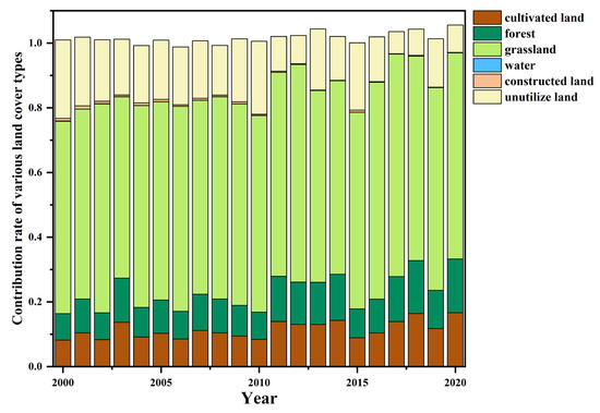
Figure 11.
Annual contribution of water conservation by land use type.
4.6.2. For Different Climatic Factors
In this study, the influence of regional PRE, PET, and LST on the changing trend of water conservation was examined according to the data scale using the formula mentioned above. The results (Figure 12) are as follows:
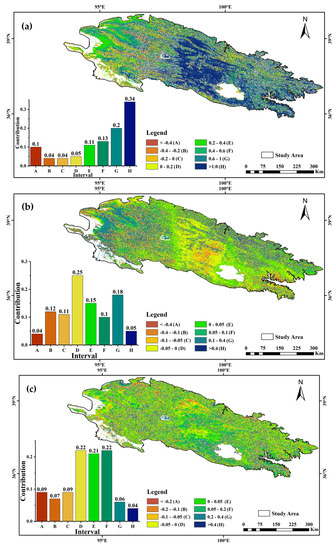
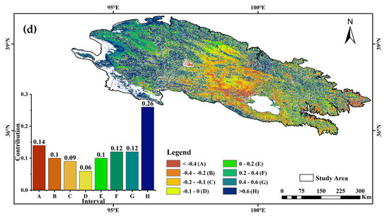
Figure 12.
Effects of climatic factors on the changing trend of water conservation from 2000 to 2020 in the QLM area: (a) map of PRE’s contribution; (b) map of PET’s contribution; (c) map of LST’s contribution; (d) map of other factors’ contribution.
- (1)
- PRE is the primary factor influencing changes in water conservation in the QLM, with a 57.711% effect on the trend unit of water conservation change. As for the geographical distribution, the PRE change trend influenced the change in the water conservation quantity in 81.997% of the research region positively. This positive influence was primarily located in southeastern and central regions. In addition, the increase in the PRE will recharge water resources and increase the amount of regional water conservation.
- (2)
- The unit average influence of the PET trend and LST trend on the trend of amount of water conservation was 1.778% and1.688%, respectively, while other factors (including land use type, subsurface factor, and slope) collectively exerted a more substantial average influence of 21.127% on the change in water conservation.
- (3)
- PET mainly played a negative role in the amount of WC, and the influence range accounted for 51.673% in the QLM, mainly distributed in the central Qinghai Lake. Additionally, the increase in the PET indicates a strong water demand from the atmosphere, resulting in decreased water conservation and a weakened water conservation service capacity.
- (4)
- The LST exhibited a negative correlation with the PRE, but its direct correlation with water conservation was not significant. Nonetheless, its positive influence spanned approximately 53.801% of the QLM, with concentrations in the western Qinghai Lake area and the northern sector of Jiuquan city. Higher surface temperatures in these regions corresponded to enhanced vegetation growth, particularly in the presence of ample PRE, indicating heightened regional water-conserving capabilities.
5. Discussion
5.1. Construction of Land Use Datasets Based on Landsat Remote Sensing Image Products
This research explored the influence changing land use patterns and climatic factors have on the water conservation service function in alpine areas against the backdrop of global warming. The land use datasets we created took both the effects of permafrost melting and changes to land patterns caused by human activity into account [72]; we also considered geological and ecological characteristics over the QLM. Consequently, a long-term land cover classification dataset was meticulously developed, with a resolution of 30 m and an accuracy of 82.5%, encompassing a time span from 2000 to 2020. Compared to existing land classification datasets, Chen et al. successfully developed a 30 m land cover data product, GlobeLand30, with an accuracy of 83.5%; however, it only included three phases: 2000, 2010, and 2020 [28]. The MCD12Q1 V6 product offers an annual global land cover product with six different classification criteria, but its resolution is 500 m. Even though there exists a land cover product with high resolution and long-time series, such as the annual China land cover dataset covering the period 1990 to 2019, which was derived by Yang and Huang, with a resolution of 30 m [73], this dataset is on a national scale, and it was not constructed based on the unique biological attributes of the QLM. In summary, the land classification dataset created in this study possesses key characteristics including long temporal coverage, high resolution, and high accuracy. It also takes into account actual factors within the research area, including frozen soil and human activities, which could impact land classification outcomes and are directly pertinent to the research focus of this paper. As a result, this dataset stands as a more fitting resource for conducting research and analysis within the QLM.
The land cover classification dataset constructed in this study also has several areas that require improvement. Notably, the dataset is susceptible to the striping effect caused by Landsat 5 and Landsat 7, as well as the influence of cloud cover and precipitation within the QLM region. These factors contribute to a reduced classification accuracy in specific years. Additionally, the relatively limited number of classification categories raises concerns regarding the potential influence of paddy fields within the cultivated land category on their actual contribution to water conservation. Moreover, the effects glaciers and permafrost have on WC within the unutilized land category warrant additional research and investigation.
5.2. Spatial and Temporal Evolution of Regional Water Conservation Function
The QLM have a multiyear average total water conservation content of 78.08 × 10⁸ m3 and a unit average water conservation of 47.52 mm. Both water production and water conservation showed similar trends in the QLM, with an overall increasing trend in the northwestern, central, and southeastern regions and a decreasing trend near Hala Lake. In addition to climate change factors, this was also related to the adoption of local anthropogenic grazing and subsequent ecological preservation and restoration projects. Vegetation cover emerged as a pivotal factor contributing to the reduction in surface runoff, thus exerting a discernible impact on the water conservation trend within the QLM.
The amount of multiyear water conservation in the QLM showed significant spatial variations, with a gradual increase in the distribution trend from the northwest to southeast, which coincided with the distribution trend of the PRE. Both water production and water conservation showed a significant increase in the southeast of Qinghai Lake and a decrease in the northwest of Hala Lake. This may be due to the fact that the LUTs in the southeast of Qinghai Lake were mainly distributed forest, cultivated land, and grassland with strong water conservation capacity and good vegetation cover, which can greatly reduce the water loss and improve the soil texture, and the regional conservation capacity is good; whereas the northwest of Hala Lake mainly distributes extensive permafrost and glacial snow, and with the global warming in recent years, glaciers have melted, which leads to an increase in surface runoff, so the soil water storage capacity of the northwest region is weakened.
5.3. Analysis of the Water-Conserving Functions of Different Land Use Types
The QLM research area’s land cover types were grouped into six key categories in this study: cultivated land, forest, grassland, water bodies, construction land, and unutilized land. The unit average water conservation amount of each LUT was compared to assess their water conservation capacity. The results demonstrate that forest land exhibits a stronger water conservation capacity, while grassland contributes the most to the total water volume in the QLM, accounting for 62.239%. The QLM are covered with characteristic Qinghai spruce, Qilian round forest, mountain poplar, etc. The forest land provides water to the atmosphere by means of evapotranspiration while consuming water, thus facilitating the transport of water and PRE on regional and even global scales [74,75]. The well-developed root systems and extensive coverage of grasslands in the alpine regions of the QLM, coupled with their vast size, play a vital role in promoting the growth of the QLM’s water-conserving capacity as well. The remaining land cover types are mainly because of fewer crops and shallower root systems, rainfall is easily lost through excessive runoff and infiltration on shallow-rooted soils [76], and surface runoff and evapotranspiration are greater, so the land has a poor water-conserving capacity. From the results of the land transfer matrix, it is evident that ecological protection measures have been insisted on in the study area, such as returning farmland into forests and pasture into grassland for many years, which has greatly improved the situation of serious soil erosion in the Qilian Mountain region [77,78] and greatly increased the area of grassland, which provides a guarantee of the whole ecosystem’s water source containment service function [40].
It is important to note the trade-off between urban land expansion and the reduction in agricultural land. Therefore, it is recommended to impose strict controls on urban expansion while focusing on strengthening the protection and quality improvement of agricultural and ecological land.
5.4. Key Climatic Drivers of Regional Water-Conserving Functions and Summary
The water conservation capacity of the study area exhibits greater sensitivity to PRE factors than to PET and LST. Intense rainfall is beneficial for most soil and cover types to overcome water deficits, increasing drainage while reducing detained water in the soil [79].
PCAs were conducted to examine the relationship between water conservation in the QLM and PRE, PET, and LST. It was found that the central part of the QLM had a significant positive correlation with PRE, which was mainly covered with alpine meadows, with deeper roots, improving the soil’s water conservation capacity and reducing soil gaps. In addition, this region also receives ample PRE, which promotes plant growth. Good vegetation can also effectively maintain water and improve the water conservation capacity.
Furthermore, the results also found a negative correlation between water conservation capacity and the amount of PET, as well as LST. In the area with a greater amount of evapotranspiration, the gap in the subsurface was larger, the soil humidity was small, and the water-conserving capacity was poorer. The hydrological regulation function of alpine meadows is primarily affected by soil temperature. This may be attributed to the fact that the soil water potential is in a high-pressure head range during the growing season, resulting in soil water conservation mainly from soil physics and root electrostatic adsorption. As the soil temperature increases, the surface tension of the water decreases, increasing the specific water capacity and the rates of both moisture absorption and evaporation [80].
In summary, both LUT and climate change exert significant impacts on watershed runoff volume, although climate change emerges as the more influential factor in water conservation when compared to land use change [21,81]. This observation stems from the fact that PRE, as an immediate source of regional water, directly affects water conservation, sinks, and stagnant water within the conservation process. Conversely, land use types, alongside other factors like slope and subsurface characteristics, primarily influence surface runoff dynamics. Consequently, regions with higher total water conservation tend to concentrate in the eastern QLM, where robust vegetation cover and ample precipitation prevail.
5.5. Shortcomings and Prospects of This Study
This paper presents a simulation and assessment of the water conservation service function in the QLM using the InVEST model. Although the model is widely used and offers convenient training processes [82], it was developed in the United States and may not fully capture the specific natural environmental conditions of the study area in this paper. Furthermore, hydrological research is more inclined to the longitudinal water changes of the unit [68,83]. Considering the vastness of the QLM and the complex structure of the ecosystem, the driving elements are highly correlated. Some parameters used in this study have not been examined by field surveys and monitoring data. Therefore, it is significant to acknowledge that the conclusions of this study may contain inherent errors and uncertainties, which may affect the accuracy of the final findings. Future studies should prioritize localizing the model and validating its parameters to enhance the simulation’s accuracy, incorporating field observations and monitoring data specific to study area of the Qilian Mountains for a more reliable representation of actual conditions.
The land classification dataset used in this study was based on Landsat data and trained and processed on its own. However, the categorization of wetlands as water bodies and glacial snow as unutilized land without a separate classification may result in the loss of detail in hydrological analyses [84]. Additionally, environmental heterogeneity, such as less commonly distributed land use types or fluctuations in topographic slopes, should be further investigated and improved in future studies to enhance the accuracy and comprehensiveness of the analysis.
In this study, the analysis of the driving forces focused on major meteorological factors, including PRE, PET, and LST. However, water conservation services are subject to multiplied factors such as meteorological conditions, soil type, vegetation, atmosphere, and underlying factors. The driving mechanism is more complex, and the selection of multifactorial driving indexes needs to be further optimized [17]. In the trend attribution analysis, which looked at the impacts of a water-sourcing trend caused by the trend changes in the meteorological factors, this study employed the approach of expressing trend changes in full differential form to examine the impacts of each meteorological factor. While this method helps to elucidate the influence of individual factors, it may overlook the detailed variability of climatic factors during the evolution process [85].
In future research, the correlation between underlying surface conditions, including slope and soil moisture, as well as various factors, should be further considered. This will not only facilitate a deeper understanding of the mechanism of the driving force of the water-conserving function of the study area but also provide a theoretical foundation for relevant ecological construction development for concerned departments.
The findings of this study generally indicate that pertinent departments should focus on protecting the vegetation in the northwest QLM and plant forests and alpine meadows with deep roots while taking the local soil and climatic conditions into consideration. Alpine regions should be developed in accordance with local needs and on the basis of sustainable development, vigorously carrying out the work of restoring natural land, scientifically planning the development of animal husbandry, paying attention to regional protection during rational development, and minimizing the harm that human activities cause to the permafrost degradation area through the establishment of nature reserves and other means.
6. Conclusions
Water conservation serves as a pivotal ecological service function, wielding significant influence over the sustainable evolution of regional hydrology. In this study, the InVEST model was utilized to estimate multiyear water conservation within the QLM basin. We conducted a comprehensive analysis of the spatial and temporal trends in regional multiyear water conservation employing various methodologies, including the Theil–Sen median trend and Mann–Kendall method, coefficient of variation assessment, and Hurst Index. Furthermore, we used partial correlation analysis and contribution analysis to discern the primary drivers influencing regional water conservation and to quantify their respective impacts. Our key findings are as follows.
Firstly, the water conservation function in the QLM exhibited significant spatial variability, gradually increasing from the northwest to the southeast. In terms of the different land types, the forest unit had the highest water conservation capacity, whereas the grassland contributed the most to the overall water conservation in the research region.
According to the examination of the driving factors, PRE was the most significant factor influencing the amount of water retained in the studied region. Additionally, PET and LST were found to be predominantly negatively correlated with water conservation. These findings indicate that changes in climatic factors have had a significant impact on the water conservation dynamics of the studied area.
Contribution analyses demonstrate that climate change and land use change, driven by multiple ecological restoration projects, collectively influence water services. These findings align with those of previous studies. With the ongoing trend of global warming, surface temperatures are rising, and the melting of glacial permafrost persists. Consequently, managing water resources necessitates a comparison between available water resources and the anticipated demand for accurate water resources, which is critical for efficient water resource management and distribution.
Given the intricate nature of climate change and the continual shifts in regional soil diversity, hydrological patterns, and landscape factors, it is imperative for governmental and relevant departments to prioritize water recycling and demand management in water resource allocation. It is also essential to carefully weigh the relationship between ecological and socioeconomic benefits, as well as short-term and long-term gains.
In summary, this study provides invaluable insight into the spatiotemporal dynamics and key drivers of water-conservation functions in the QLM. The findings emphasize the need for effective water resource management strategies that account for the complexities of the changing environment and promote sustainable development.
Author Contributions
Conceptualization, J.S. and M.W.; methodology, J.S. and M.W.; software, J.S. and C.N.; validation, J.S. and C.N.; formal analysis, J.S.; investigation, J.S.; resources, J.S.; data curation, J.S. and C.N.; writing—original draft preparation, J.S. and C.N.; writing—review and editing, J.S., C.N. and M.W.; visualization, J.S. and C.N.; supervision, M.W.; project administration, J.S.; funding acquisition, M.W. All authors have read and agreed to the published version of the manuscript.
Funding
This research was supported in part by the National College Students’ innovation and entrepreneurship training program (202210491064, 202310491029, S202210491062) and the Strategic Priority Research Program of the Chinese Academy of Sciences (XDA19090300), and it was funded by the National Natural Science Foundation of China, under grants: 61801443 and 41801348.
Data Availability Statement
Not applicable.
Conflicts of Interest
The authors declare no conflict of interest.
References
- Li, G.; Jiang, C.; Zhang, Y.; Jiang, G. Whether land greening in different geomorphic units are beneficial to water yield in the Yellow River Basin? Ecol. Indic. 2021, 120, 106926. [Google Scholar] [CrossRef]
- Biao, Z.; Wenhua, L.; Gaodi, X.; Yu, X. Water conservation of forest ecosystem in Beijing and its value. Ecol. Econ. 2010, 69, 1416–1426. [Google Scholar] [CrossRef]
- Cao, S.; Zhang, J.; Chen, L.; Zhao, T. Ecosystem water imbalances created during ecological restoration by afforestation in China, and lessons for other developing countries. J. Environ. Manag. 2016, 183, 843–849. [Google Scholar] [CrossRef]
- Zhang, B.; Song, X.; Zhang, Y.; Han, D.; Tang, C.; Yu, Y.; Ma, Y. Hydrochemical characteristics and water quality assessment of surface water and groundwater in Songnen plain, Northeast China. Water Res. 2012, 46, 2737–2748. [Google Scholar] [CrossRef]
- Huang, Z.; Liu, X.; Sun, S.; Tang, Y.; Yuan, X.; Tang, Q. Global assessment of future sectoral water scarcity under adaptive inner-basin water allocation measures. Sci. Total Environ. 2021, 783, 146973. [Google Scholar] [CrossRef]
- Liu, J.; Yang, W. Water management. Water sustainability for China and beyond. Science 2012, 337, 649–650. [Google Scholar] [CrossRef] [PubMed]
- Mekonnen, M.M.; Hoekstra, A.Y. Four billion people facing severe water scarcity. Sci. Adv. 2016, 2, e1500323. [Google Scholar] [CrossRef]
- Scordo, F.; Lavender, T.; Seitz, C.; Perillo, V.; Rusak, J.; Piccolo, M.; Perillo, G. Modeling Water Yield: Assessing the Role of Site and Region-Specific Attributes in Determining Model Performance of the InVEST Seasonal Water Yield Model. Water 2018, 10, 1496. [Google Scholar] [CrossRef]
- Xue, J.; Li, Z.; Feng, Q.; Miao, C.; Deng, X.; Di, Z.; Ye, A.; Gong, W.; Zhang, B.; Gui, J. Spatiotemporal variation characteristics of water conservation amount in the Qilian Mountains from 1980 to 2017. J. Glaciol. Geocryol. 2022, 44, 1–13. [Google Scholar]
- Bai, Y.; Ochuodho, T.O.; Yang, J. Impact of land use and climate change on water-related ecosystem services in Kentucky, USA. Ecol. Indic. 2019, 102, 51–64. [Google Scholar] [CrossRef]
- Baker, T.J.; Miller, S.N. Using the Soil and Water Assessment Tool (SWAT) to assess land use impact on water resources in an East African watershed. J. Hydrol. 2013, 486, 100–111. [Google Scholar] [CrossRef]
- Hoyer, R.; Chang, H. Assessment of freshwater ecosystem services in the Tualatin and Yamhill basins under climate change and urbanization. Appl. Geogr. 2014, 53, 402–416. [Google Scholar] [CrossRef]
- Leonard, L. Using machine learning models to predict and choose meshes reordered by graph algorithms to improve execution times for hydrological modeling. Environ. Model. Softw. 2019, 119, 84–98. [Google Scholar] [CrossRef]
- Krysanova, V.; Wechsung, F.; Arnold, J.; Srinivasan, R.; Williams, J. PIK Report Nr. 69 “SWIM (Soil and Water Integrated Model), User Manual”; Potsdam Institute for Climate Impact Research (PIK): Potsdam, Germany, 2002; 39p. [Google Scholar]
- Refsgaard, J.; Storm, B.; Singh, V. MIKE SHE. Comput. Models Watershed Hydrol. 1995, 1, 809–846. [Google Scholar]
- Ajaz Ahmed, M.A.; Abd-Elrahman, A.; Escobedo, F.J.; Cropper, W.P., Jr.; Martin, T.A.; Timilsina, N. Spatially-explicit modeling of multi-scale drivers of aboveground forest biomass and water yield in watersheds of the Southeastern United States. J. Environ. Manag. 2017, 199, 158–171. [Google Scholar] [CrossRef]
- Hu, W.; Li, G.; Gao, Z.; Jia, G.; Wang, Z.; Li, Y. Assessment of the impact of the Poplar Ecological Retreat Project on water conservation in the Dongting Lake wetland region using the InVEST model. Sci. Total Environ. 2020, 733, 139423. [Google Scholar] [CrossRef]
- Yu, Y.; Sun, X.; Wang, J.; Zhang, J. Using InVEST to evaluate water yield services in Shangri-La, Northwestern Yunnan, China. PeerJ 2022, 10, e12804. [Google Scholar] [CrossRef] [PubMed]
- Moreira, M.; Fonseca, C.; Vergílio, M.; Calado, H.; Gil, A. Spatial assessment of habitat conservation status in a Macaronesian island based on the InVEST model: A case study of Pico Island (Azores, Portugal). Land Use Policy 2018, 78, 637–649. [Google Scholar] [CrossRef]
- Moitellam, R. Book Reviews. Med. J. Aust. 1962, 1, 274–275. [Google Scholar] [CrossRef]
- Aneseyee, A.B.; Soromessa, T.; Elias, E.; Noszczyk, T.; Feyisa, G.L. Evaluation of Water Provision Ecosystem Services Associated with Land Use/Cover and Climate Variability in the Winike Watershed, Omo Gibe Basin of Ethiopia. Environ. Manag. 2022, 69, 367–383. [Google Scholar] [CrossRef]
- Miralles, D.G.; van den Berg, M.J.; Gash, J.H.; Parinussa, R.M.; de Jeu, R.A.M.; Beck, H.E.; Holmes, T.R.H.; Jiménez, C.; Verhoest, N.E.C.; Dorigo, W.A.; et al. El Niño–La Niña cycle and recent trends in continental evaporation. Nat. Clim. Chang. 2013, 4, 122–126. [Google Scholar] [CrossRef]
- Matios, E.; Burney, J. Ecosystem Services Mapping for Sustainable Agricultural Water Management in California’s Central Valley. Environ. Sci. Technol. 2017, 51, 2593–2601. [Google Scholar] [CrossRef]
- Yohannes, H.; Soromessa, T.; Argaw, M.; Dewan, A. Impact of landscape pattern changes on hydrological ecosystem services in the Beressa watershed of the Blue Nile Basin in Ethiopia. Sci. Total Environ. 2021, 793, 148559. [Google Scholar] [CrossRef] [PubMed]
- Wu, Q.; Song, J.; Sun, H.; Huang, P.; Jing, K.; Xu, W.; Wang, H.; Liang, D. Spatiotemporal variations of water conservation function based on EOF analysis at multi time scales under different ecosystems of Heihe River Basin. J. Environ. Manag. 2023, 325, 116532. [Google Scholar] [CrossRef] [PubMed]
- Eingruber, N.; Korres, W. Climate change simulation and trend analysis of extreme precipitation and floods in the mesoscale Rur catchment in western Germany until 2099 using Statistical Downscaling Model (SDSM) and the Soil & Water Assessment Tool (SWAT model). Sci. Total Environ. 2022, 838, 155775. [Google Scholar] [CrossRef]
- Li, M.; Liang, D.; Xia, J.; Song, J.; Cheng, D.; Wu, J.; Cao, Y.; Sun, H.; Li, Q. Evaluation of water conservation function of Danjiang River Basin in Qinling Mountains, China based on InVEST model. J. Environ. Manag. 2021, 286, 112212. [Google Scholar] [CrossRef]
- Chen, J.; Liao, A.P.; Chen, J. Global 30m land cover remote sensing data product -GlobeLand30. Geomat. World 2017, 24, 1–8. [Google Scholar]
- Viviroli, D.; Dürr, H.H.; Messerli, B.; Meybeck, M.; Weingartner, R. Mountains of the world, water towers for humanity: Typology, mapping, and global significance. Water Resour. Res. 2007, 43, W07447. [Google Scholar] [CrossRef]
- Qian, D.; Du, Y.; Li, Q.; Guo, X.; Cao, G. Alpine grassland management based on ecosystem service relationships on the southern slopes of the Qilian Mountains, China. J. Environ. Manag. 2021, 288, 112447. [Google Scholar] [CrossRef]
- Yang, L.; Feng, Q.; Adamowski, J.F.; Alizadeh, M.R.; Yin, Z.; Wen, X.; Zhu, M. The role of climate change and vegetation greening on the variation of terrestrial evapotranspiration in northwest China’s Qilian Mountains. Sci. Total Environ. 2021, 759, 143532. [Google Scholar] [CrossRef]
- Wang, H.; Xiong, X.; Wang, K.; Li, X.; Hu, H.; Li, Q.; Yin, H.; Wu, C. The effects of land use on water quality of alpine rivers: A case study in Qilian Mountain, China. Sci. Total Environ. 2023, 875, 162696. [Google Scholar] [CrossRef] [PubMed]
- Zhang, M.; Jia, W.; Zhu, G.; Shi, Y.; Zhang, Z.; Xiong, H.; Yang, L.; Zhang, F. Contribution of recycled moisture to precipitation and its influencing factors in the subalpine zone of Qilian Mountains. Environ. Sci. Pollut. Res. Int. 2022, 29, 45947–45959. [Google Scholar] [CrossRef] [PubMed]
- Li, Z.; Yuan, R.; Feng, Q.; Zhang, B.; Lv, Y.; Li, Y.; Wei, W.; Chen, W.; Ning, T.; Gui, J.; et al. Climate background, relative rate, and runoff effect of multiphase water transformation in Qilian Mountains, the third pole region. Sci. Total Environ. 2019, 663, 315–328. [Google Scholar] [CrossRef]
- Liu, Y.; Liu, X.; Zhao, C.; Wang, H.; Zang, F. The trade-offs and synergies of the ecological-production-living functions of grassland in the Qilian mountains by ecological priority. J. Environ. Manag. 2023, 327, 116883. [Google Scholar] [CrossRef]
- Ma, Z.; Gong, J.; Hu, C.; Lei, J. An integrated approach to assess spatial and temporal changes in the contribution of the ecosystem to sustainable development goals over 20 years in China. Sci. Total Environ. 2023, 903, 166237. [Google Scholar] [CrossRef] [PubMed]
- Huang, F.; Liu, L.; Gao, J.; Yin, Z.; Zhang, Y.; Jiang, Y.; Zuo, L.; Fang, W. Effects of extreme drought events on vegetation activity from the perspectives of meteorological and soil droughts in southwestern China. Sci. Total Environ. 2023, 903, 166562. [Google Scholar] [CrossRef] [PubMed]
- Li, G.; Chen, W.; Zhang, X.; Bi, P.; Yang, Z.; Shi, X.; Wang, Z. Spatiotemporal dynamics of vegetation in China from 1981 to 2100 from the perspective of hydrothermal factor analysis. Environ. Sci. Pollut. Res. Int. 2022, 29, 14219–14230. [Google Scholar] [CrossRef] [PubMed]
- Song, W.; Song, W. Cropland fallow reduces agricultural water consumption by 303 million tons annually in Gansu Province, China. Sci. Total Environ. 2023, 879, 163013. [Google Scholar] [CrossRef]
- Sun, D.; Liang, Y.; Peng, S. Scenario simulation of water retention services under land use/cover and climate changes: A case study of the Loess Plateau, China. J. Arid Land 2022, 14, 390–410. [Google Scholar] [CrossRef]
- Ding, Y.; Peng, S. Spatiotemporal trends and attribution of drought across China from 1901–2100. Sustainability 2020, 12, 477. [Google Scholar] [CrossRef]
- Peng, S.; Gang, C.; Cao, Y.; Chen, Y. Assessment of climate change trends over the loess plateau in china from 1901 to 2100. Int. J. Climatol. 2017, 38, 2250–2264. [Google Scholar] [CrossRef]
- Peng, S.; Ding, Y.; Liu, W.; Li, Z. 1 km monthly temperature and precipitation dataset for China from 1901 to 2017. Earth Syst. Sci. Data 2019, 11, 1931–1946. [Google Scholar] [CrossRef]
- Peng, S.; Ding, Y.; Wen, Z.; Chen, Y.; Cao, Y.; Ren, J. Spatiotemporal change and trend analysis of potential evapotranspiration over the Loess Plateau of China during 2011–2100. Agric. For. Meteorol. 2017, 233, 183–194. [Google Scholar] [CrossRef]
- Peng, S. 1-km Monthly Precipitation Dataset for China (1901–2022); A Big Earth Data Platform for Three Poles: Lanzhou, China, 2020. [Google Scholar] [CrossRef]
- Ding, Y.; Peng, S. Spatiotemporal change and attribution of potential evapotranspiration over China from 1901 to 2100. Theor. Appl. Climatol. 2021, 145, 79–94. [Google Scholar] [CrossRef]
- Peng, S. 1 km Monthly Potential Evapotranspiration Dataset in China (1901–2022); National Tibetan Plateau Data Center: Beijing, China, 2022. [CrossRef]
- Miralles, D.G.; Holmes, T.R.H.; De Jeu, R.A.M.; Gash, J.H.; Meesters, A.G.C.A.; Dolman, A.J. Global land-surface evaporation estimated from satellite-based observations. Hydrol. Earth Syst. Sci. 2011, 15, 453–469. [Google Scholar] [CrossRef]
- Martens, B.; Miralles, D.G.; Lievens, H.; van der Schalie, R.; de Jeu, R.A.M.; Fernández-Prieto, D.; Beck, H.E.; Dorigo, W.A.; Verhoest, N.E.C. GLEAM v3: Satellite-based land evaporation and root-zone soil moisture. Geosci. Model Dev. 2017, 10, 1903–1925. [Google Scholar] [CrossRef]
- Chenyang Peng, Y.S.; Wu, J.; Cao, W.; Binbin, H.E. Simulation of the permafrost distribution in the Qilian Mountains. J. Glaciol. Geocryol. 2021, 43, 158–169. [Google Scholar] [CrossRef]
- Creed, I.F.; Spargo, A.T.; Jones, J.A.; Buttle, J.M.; Adams, M.B.; Beall, F.D.; Booth, E.G.; Campbell, J.L.; Clow, D.; Elder, K.; et al. Changing forest water yields in response to climate warming: Results from long-term experimental watershed sites across North America. Glob. Chang. Biol. 2014, 20, 3191–3208. [Google Scholar] [CrossRef]
- Williams, C.A.; Reichstein, M.; Buchmann, N.; Baldocchi, D.; Beer, C.; Schwalm, C.; Wohlfahrt, G.; Hasler, N.; Bernhofer, C.; Foken, T.; et al. Climate and vegetation controls on the surface water balance: Synthesis of evapotranspiration measured across a global network of flux towers. Water Resour. Res. 2012, 48, W06523. [Google Scholar] [CrossRef]
- Jiang, C.; Li, D.; Wang, D.; Zhang, L. Quantification and assessment of changes in ecosystem service in the Three-River Headwaters Region, China as a result of climate variability and land cover change. Ecol. Indic. 2016, 66, 199–211. [Google Scholar] [CrossRef]
- Wenzuo, Z. A Study on Available Water Capacity of Main Soil Types in China Based on Geographic Information System; Nanjing Agricultural University: Nanjing, China, 2003. [Google Scholar]
- Redhead, J.W.; Stratford, C.; Sharps, K.; Jones, L.; Ziv, G.; Clarke, D.; Oliver, T.H.; Bullock, J.M. Empirical validation of the InVEST water yield ecosystem service model at a national scale. Sci. Total Environ. 2016, 569–570, 1418–1426. [Google Scholar] [CrossRef] [PubMed]
- Hu, W.; Li, G.; Li, Z. Spatial and temporal evolution characteristics of the water conservation function and its driving factors in regional lake wetlands—Two types of homogeneous lakes as examples. Ecol. Indic. 2021, 130, 108069. [Google Scholar] [CrossRef]
- Wu, C.; Qiu, D.; Gao, P.; Mu, X.; Zhao, G. Application of the InVEST model for assessing water yield and its response to precipitation and land use in the Weihe River Basin, China. J. Arid Land 2022, 14, 426–440. [Google Scholar] [CrossRef]
- Zeng, Q.; Liu, D.; An, S. Decoupled diversity patterns in microbial geographic distributions on the arid area (the Loess Plateau). Catena 2021, 196, 104922. [Google Scholar] [CrossRef]
- Budyko, M.I. The Heat Balance of the Earth’s Surface. Sov. Geogr. 2014, 2, 3–13. [Google Scholar] [CrossRef]
- Zhang, L.; Hickel, K.; Dawes, W.R.; Chiew, F.H.S.; Western, A.W.; Briggs, P.R. A rational function approach for estimating mean annual evapotranspiration. Water Resour. Res. 2004, 40, W02502. [Google Scholar] [CrossRef]
- Pan, S.; Tian, H.; Dangal, S.R.S.; Yang, Q.; Yang, J.; Lu, C.; Tao, B.; Ren, W.; Ouyang, Z. Responses of global terrestrial evapotranspiration to climate change and increasing atmospheric CO2 in the 21st century. Earth’s Future 2015, 3, 15–35. [Google Scholar] [CrossRef]
- Liu, J.; You, Y.; Li, J.; Sitch, S.; Gu, X.; Nabel, J.E.M.S.; Lombardozzi, D.; Luo, M.; Feng, X.; Arneth, A.; et al. Response of global land evapotranspiration to climate change, elevated CO2, and land use change. Agric. For. Meteorol. 2021, 311, 108663. [Google Scholar] [CrossRef]
- Zhao, L.; Xia, J.; Xu, C.-Y.; Wang, Z.; Sobkowiak, L.; Long, C. Evapotranspiration estimation methods in hydrological models. J. Geogr. Sci. 2013, 23, 359–369. [Google Scholar] [CrossRef]
- Velpuri, N.M.; Senay, G.B.; Singh, R.K.; Bohms, S.; Verdin, J.P. A comprehensive evaluation of two MODIS evapotranspiration products over the conterminous United States: Using point and gridded FLUXNET and water balance ET. Remote Sens. Environ. 2013, 139, 35–49. [Google Scholar] [CrossRef]
- Xu, T.; Guo, Z.; Xia, Y.; Ferreira, V.G.; Liu, S.; Wang, K.; Yao, Y.; Zhang, X.; Zhao, C. Evaluation of twelve evapotranspiration products from machine learning, remote sensing and land surface models over conterminous United States. J. Hydrol. 2019, 578, 124105. [Google Scholar] [CrossRef]
- Jiang, W.; Yuan, L.; Wang, W.; Cao, R.; Zhang, Y.; Shen, W. Spatio-temporal analysis of vegetation variation in the Yellow River Basin. Ecol. Indic. 2015, 51, 117–126. [Google Scholar] [CrossRef]
- Peng, J.; Shen, H.; Wu, W.; Liu, Y.; Wang, Y. Net primary productivity (NPP) dynamics and associated urbanization driving forces in metropolitan areas: A case study in Beijing City, China. Landsc. Ecol. 2015, 31, 1077–1092. [Google Scholar] [CrossRef]
- Feng, Q.; Zhao, W.; Wang, J.; Zhang, X.; Zhao, M.; Zhong, L.; Liu, Y.; Fang, X. Effects of Different Land-Use Types on Soil Erosion Under Natural Rainfall in the Loess Plateau, China. Pedosphere 2016, 26, 243–256. [Google Scholar] [CrossRef]
- Yin, L.; Tao, F.; Chen, Y.; Liu, F.; Hu, J. Improving terrestrial evapotranspiration estimation across China during 2000–2018 with machine learning methods. J. Hydrol. 2021, 600, 126538. [Google Scholar] [CrossRef]
- Or, D.; Lehmann, P. Surface Evaporative Capacitance: How Soil Type and Rainfall Characteristics Affect Global-Scale Surface Evaporation. Water Resour. Res. 2019, 55, 519–539. [Google Scholar] [CrossRef]
- Lewis, C.S.; Allen, L.N. Potential crop evapotranspiration and surface evaporation estimates via a gridded weather forcing dataset. J. Hydrol. 2017, 546, 450–463. [Google Scholar] [CrossRef]
- Pan, T.; Wu, S.H.; Dai, E.F.; Liu, Y.J. Spatiotemporal variation of water source supply service in Three Rivers Source Area of China based on InVEST model. Ying Yong Sheng Tai Xue Bao 2013, 24, 183–189. [Google Scholar] [CrossRef]
- Yang, J.; Huang, X. The 30 m annual land cover dataset and its dynamics in China from 1990 to 2019. Earth Syst. Sci. Data 2021, 13, 3907–3925. [Google Scholar] [CrossRef]
- Bennett, B.M.; Barton, G.A. The enduring link between forest cover and rainfall: A historical perspective on science and policy discussions. For. Ecosyst. 2018, 5, 5. [Google Scholar] [CrossRef]
- Ellison, D.; Futter, M.N.; Bishop, K. On the forest cover-water yield debate: From demand- to supply-side thinking. Glob. Chang. Biol. 2011, 18, 806–820. [Google Scholar] [CrossRef]
- Helman, D.; Lensky, I.M.; Yakir, D.; Osem, Y. Forests growing under dry conditions have higher hydrological resilience to drought than do more humid forests. Glob. Chang. Biol. 2017, 23, 2801–2817. [Google Scholar] [CrossRef] [PubMed]
- Jia, G.; Hu, W.; Zhang, B.; Li, G.; Shen, S.; Gao, Z.; Li, Y. Assessing impacts of the Ecological Retreat project on water conservation in the Yellow River Basin. Sci. Total Environ. 2022, 828, 154483. [Google Scholar] [CrossRef] [PubMed]
- Teo, H.C.; Raghavan, S.V.; He, X.; Zeng, Z.; Cheng, Y.; Luo, X.; Lechner, A.M.; Ashfold, M.J.; Lamba, A.; Sreekar, R.; et al. Large-scale reforestation can increase water yield and reduce drought risk for water-insecure regions in the Asia-Pacific. Glob. Chang. Biol. 2022, 28, 6385–6403. [Google Scholar] [CrossRef]
- Cuthbert, M.O.; Rau, G.C.; Ekstrom, M.; O’Carroll, D.M.; Bates, A.J. Global climate-driven trade-offs between the water retention and cooling benefits of urban greening. Nat. Commun. 2022, 13, 518. [Google Scholar] [CrossRef]
- Sharp, R.; Chaplin-kramer, R.; Wood, S.; Guerry, A.; Ricketts, T.; Nelson, E.; Ennaanay, D.; Wolny, S.; Olwero, N.; Vigerstol, K.; et al. InVEST 3.2.0 User’s Guide; The Natural Capital Project: Stanford, CA, USA; Stanford University: Stanford, CA, USA; University of Minnesota: Minneapolis, MN, USA; The Nature Conservancy: Arlington County, VA, USA; World Wildlife Fund: Gland, Switzerland, 2015. [Google Scholar]
- Ahiablame, L.; Shakya, R. Modeling flood reduction effects of low impact development at a watershed scale. J. Environ. Manag. 2016, 171, 81–91. [Google Scholar] [CrossRef]
- Agudelo, C.A.R.; Bustos, S.L.H.; Moreno, C.A.P. Modeling interactions among multiple ecosystem services. A critical review. Ecol. Model. 2020, 429, 109103. [Google Scholar] [CrossRef]
- Yeo, I.Y.; Lang, M.W.; Lee, S.; McCarty, G.W.; Sadeghi, A.M.; Yetemen, O.; Huang, C. Mapping landscape-level hydrological connectivity of headwater wetlands to downstream waters: A geospatial modeling approach—Part 1. Sci. Total Environ. 2019, 653, 1546–1556. [Google Scholar] [CrossRef]
- Wang, H.; Wang, W.J.; Liu, Z.; Wang, L.; Zhang, W.; Zou, Y.; Jiang, M. Combined effects of multi-land use decisions and climate change on water-related ecosystem services in Northeast China. J. Environ. Manag. 2022, 315, 115131. [Google Scholar] [CrossRef]
- Lessa Derci Augustynczik, A.; Yousefpour, R. Assessing the synergistic value of ecosystem services in European beech forests. Ecosyst. Serv. 2021, 49, 101264. [Google Scholar] [CrossRef]
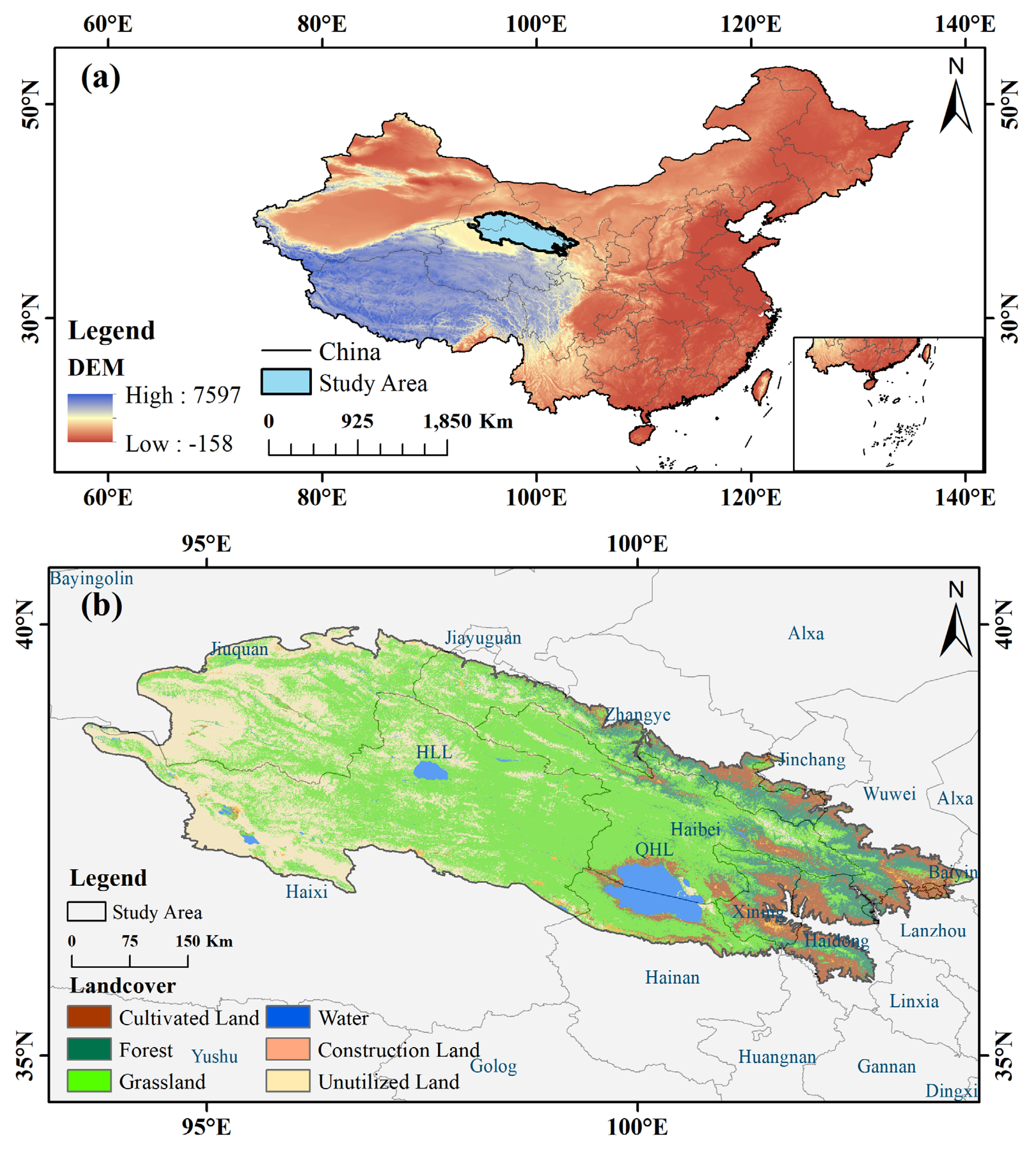
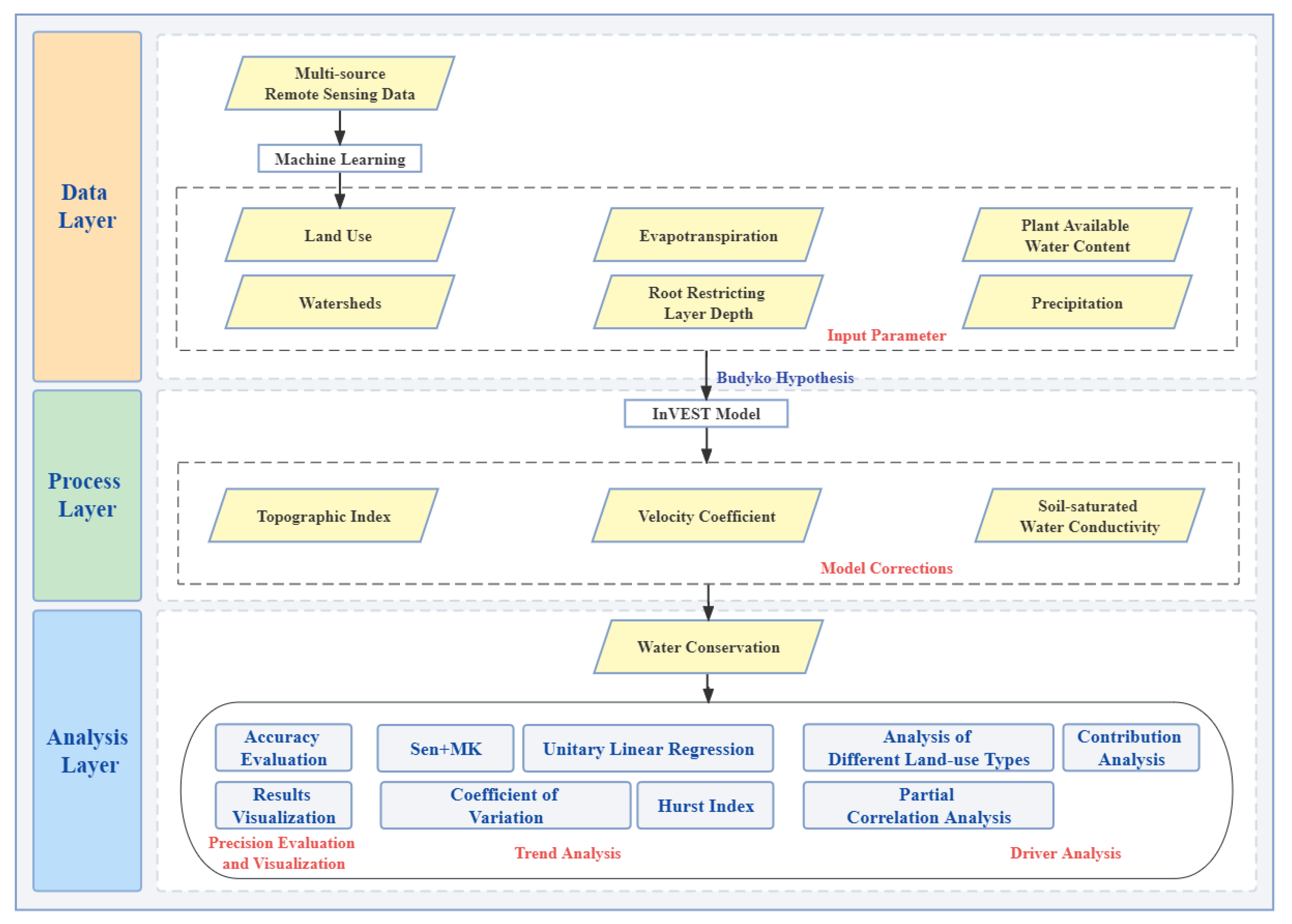
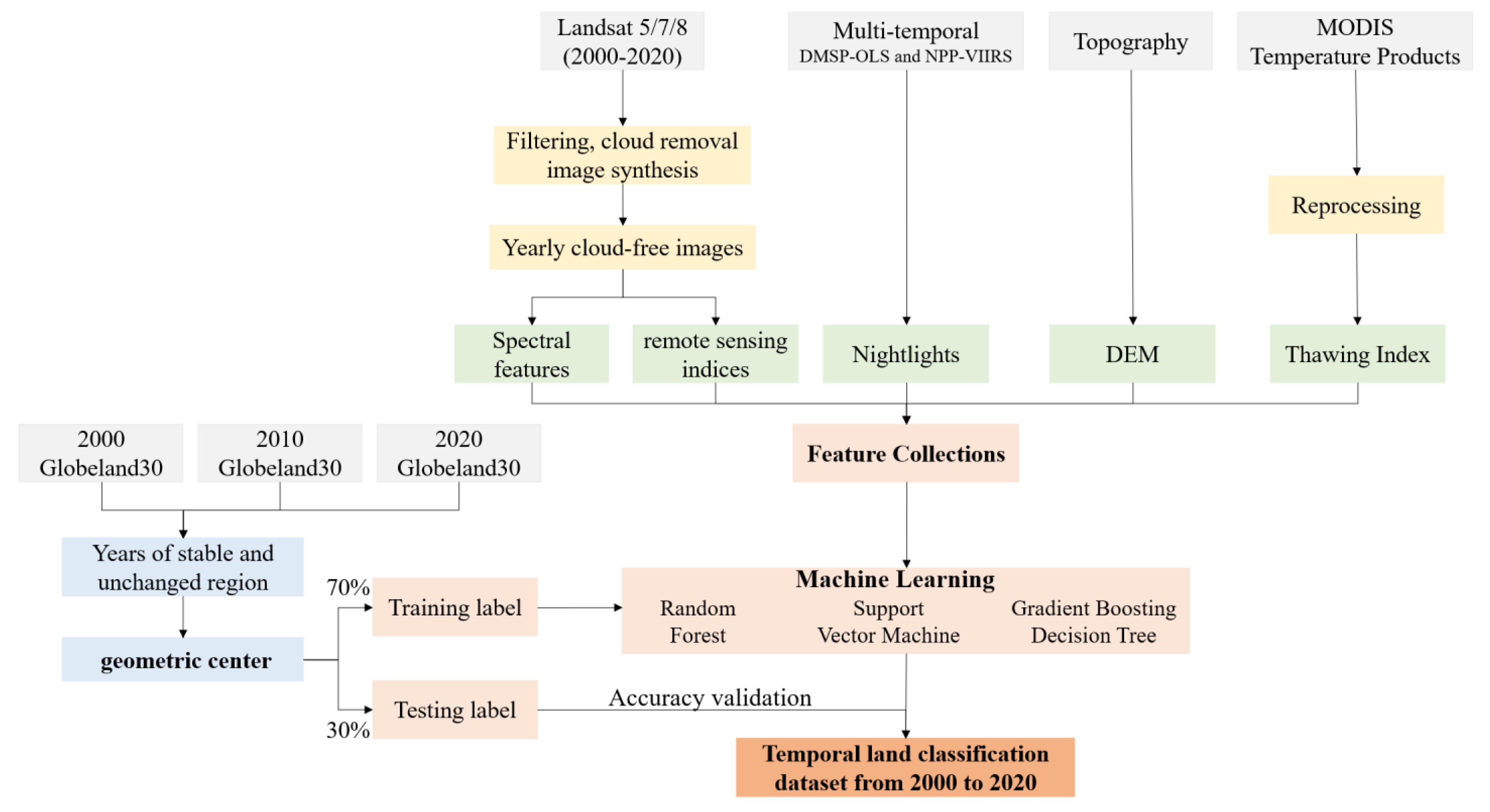
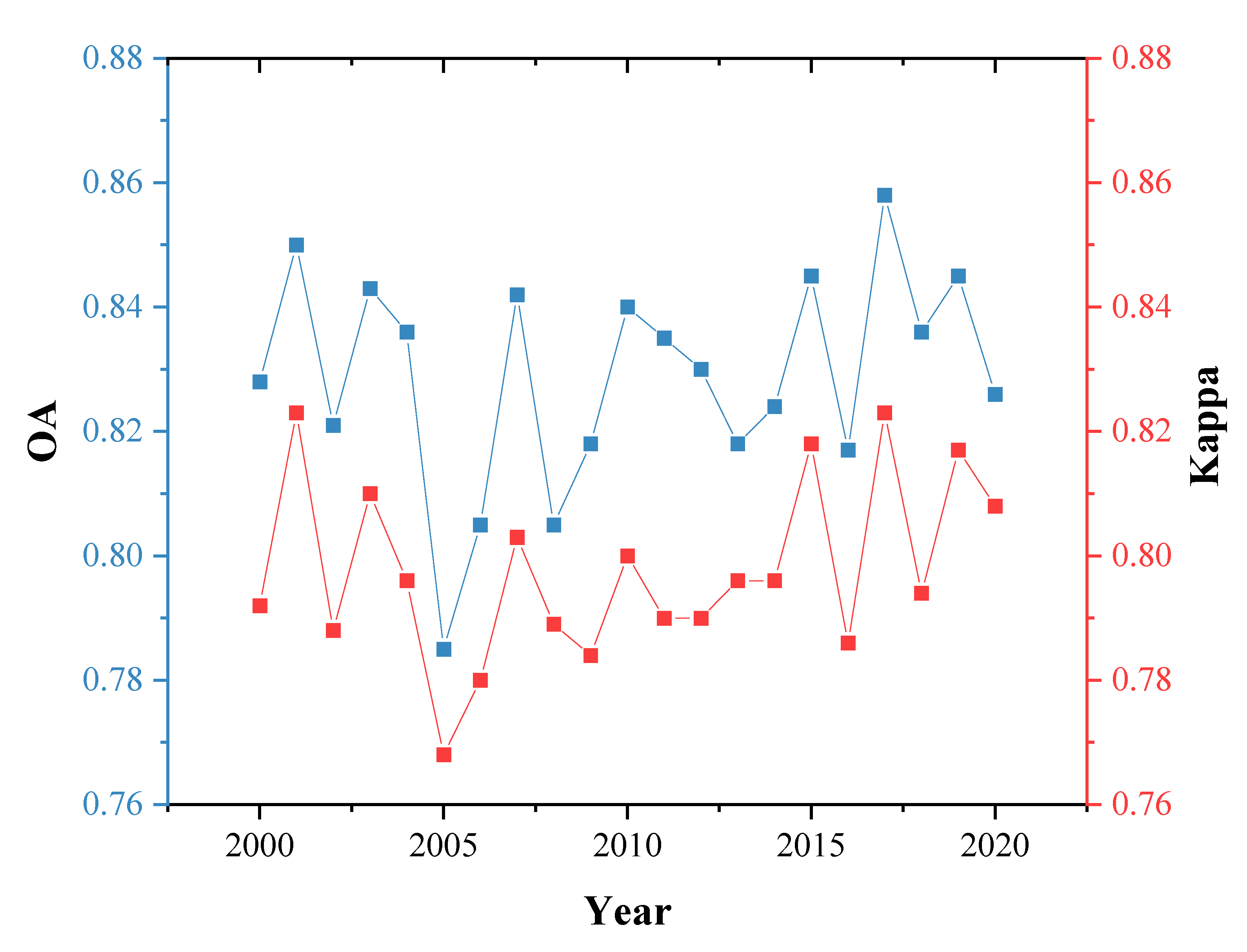
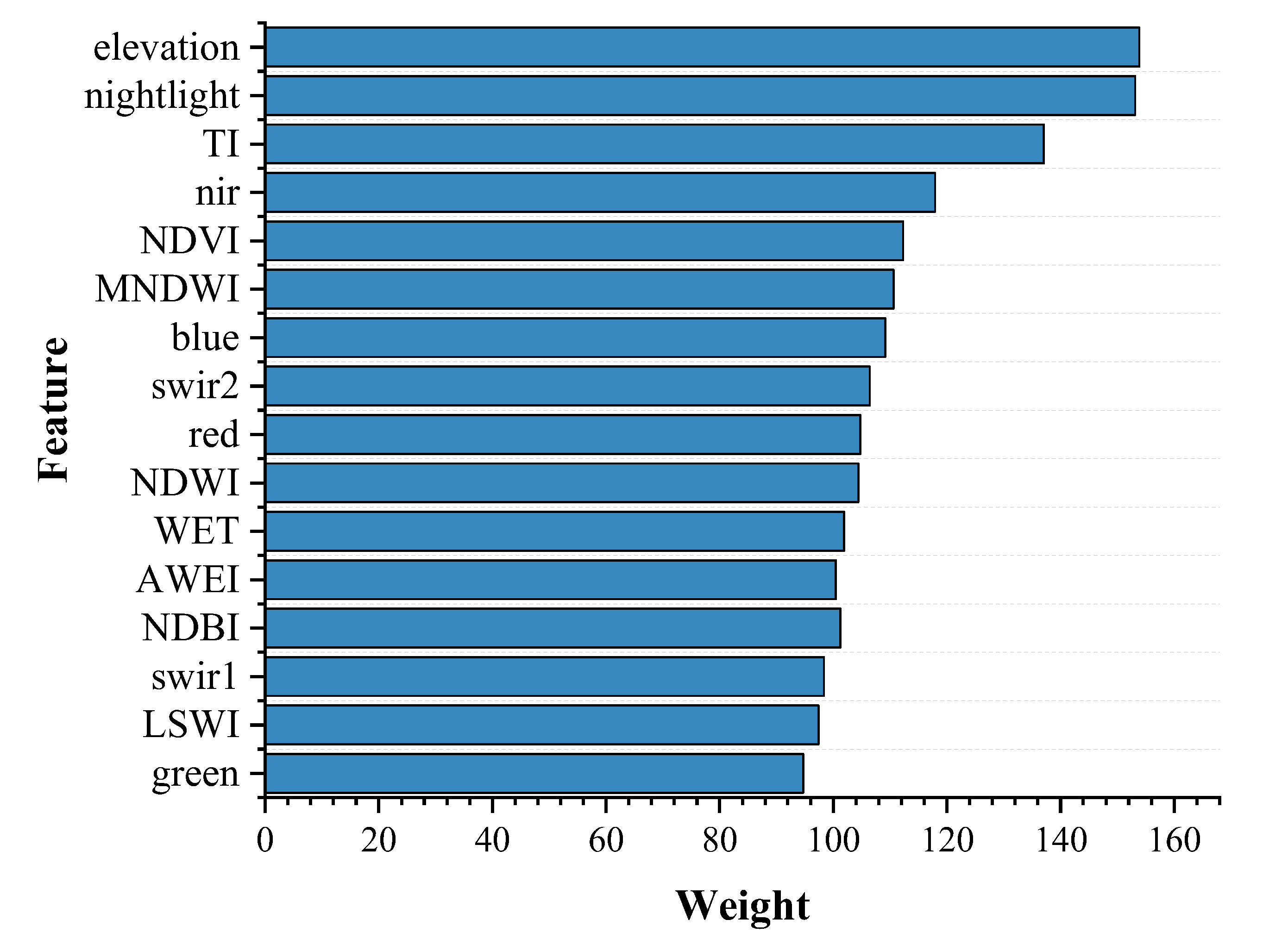


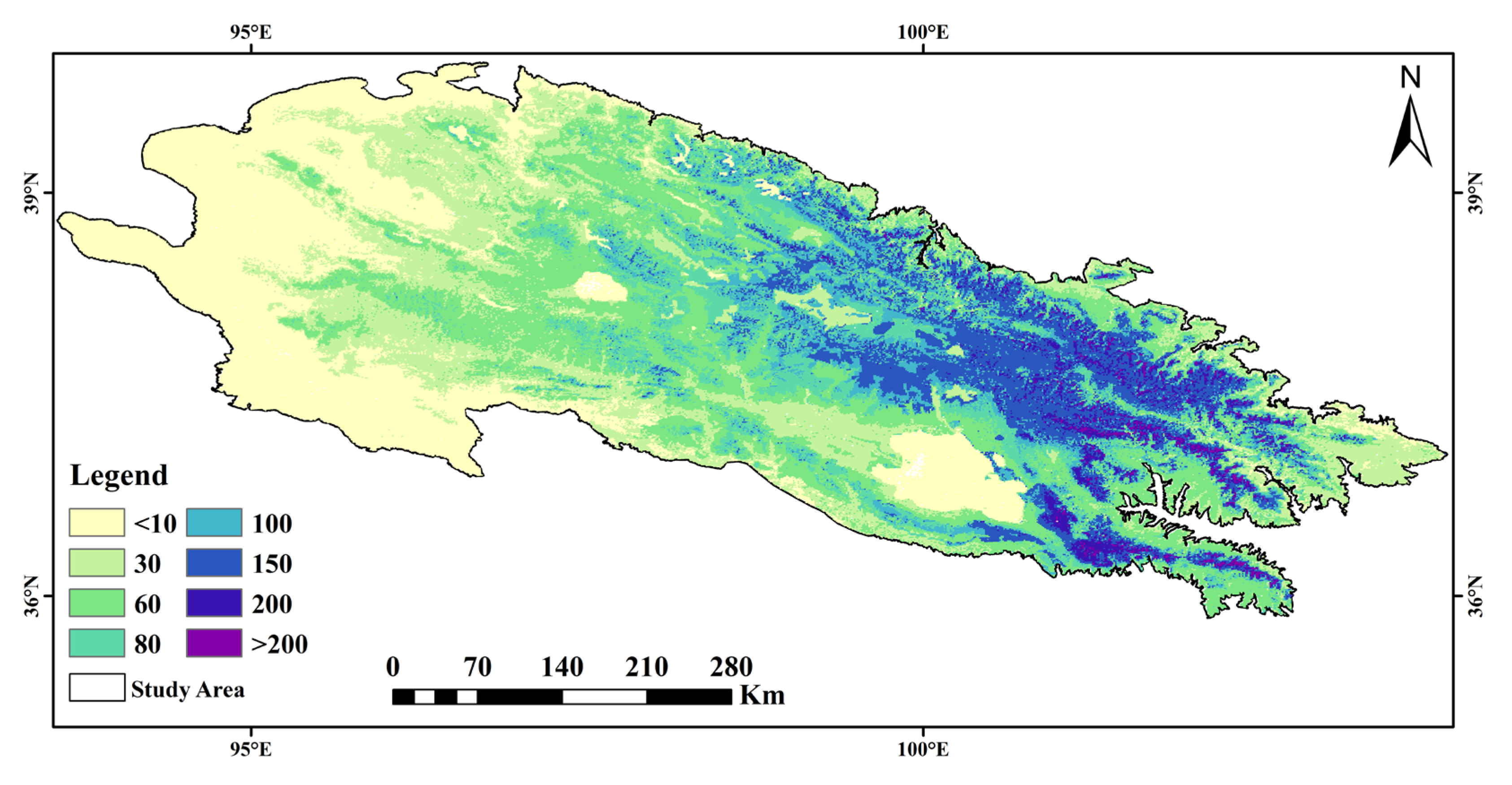
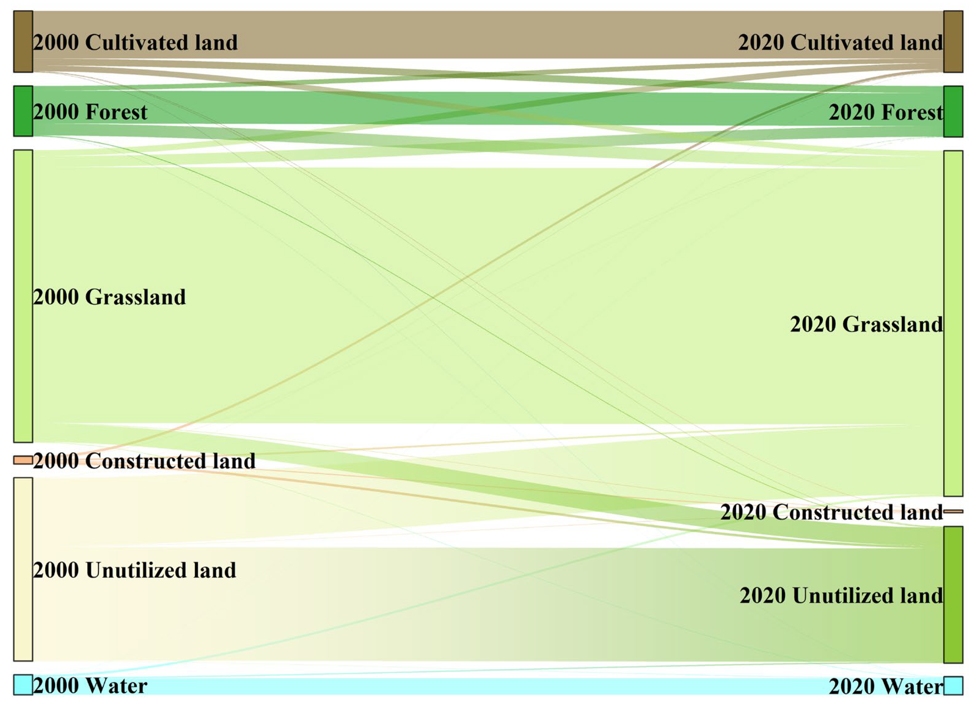
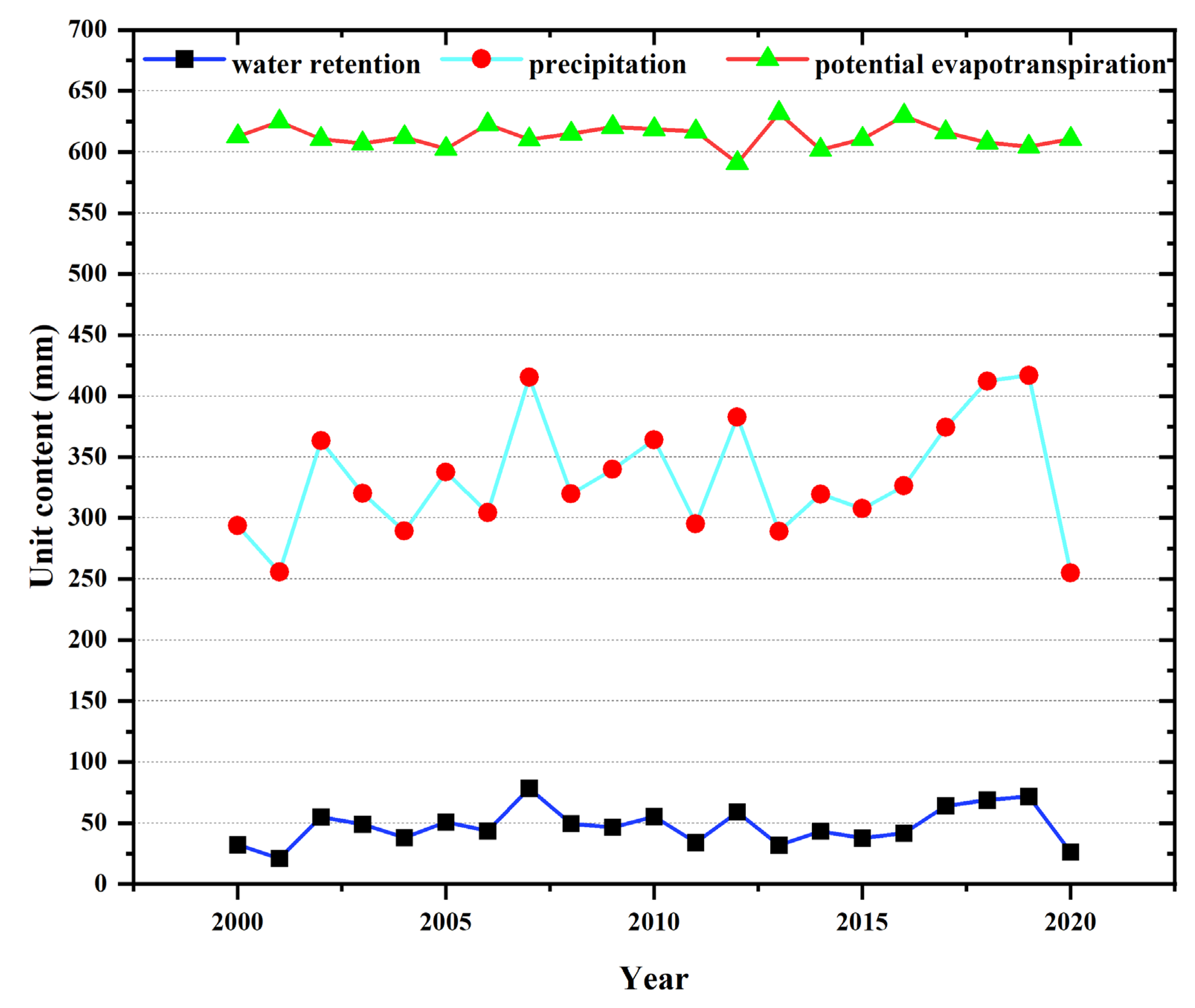
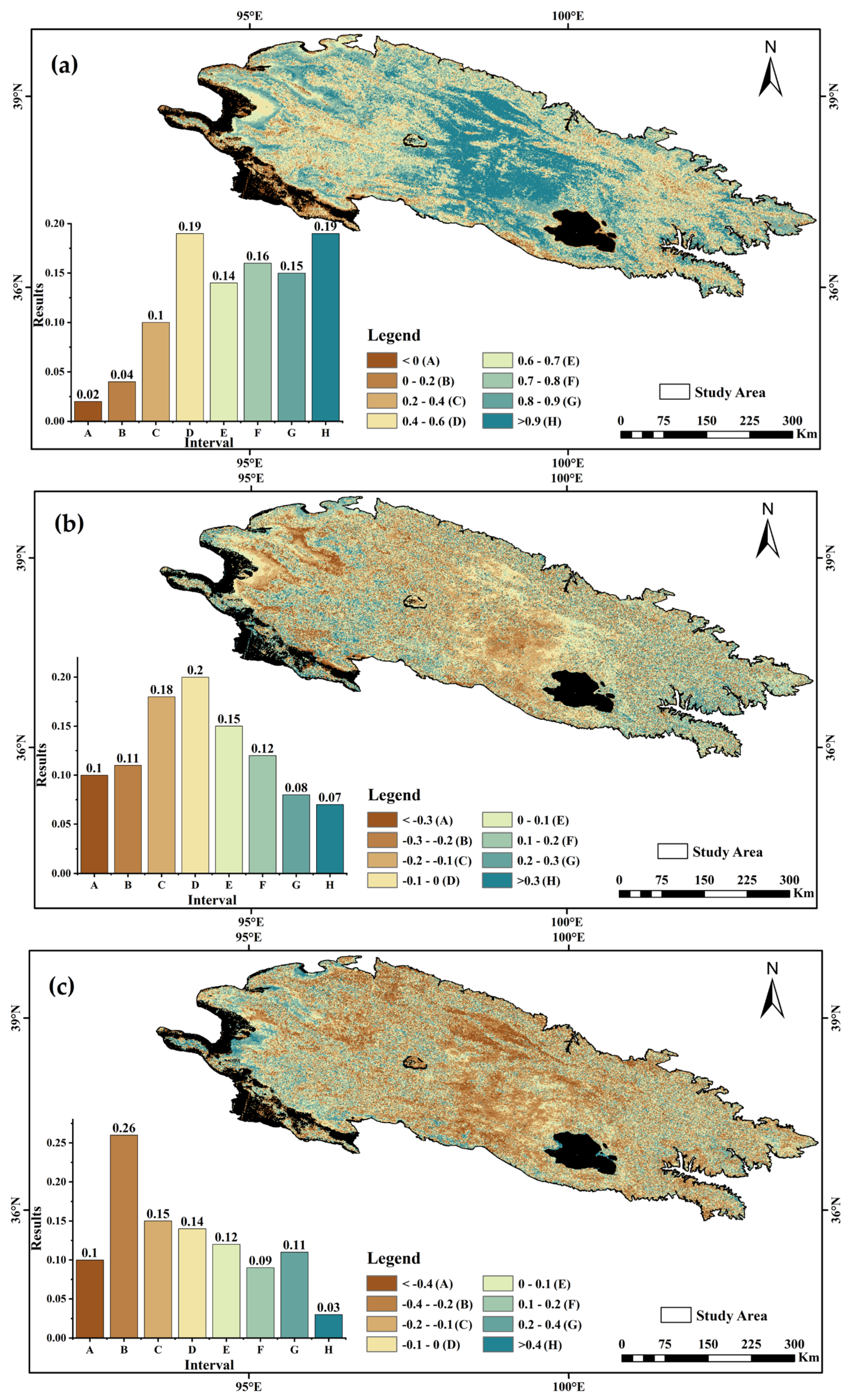
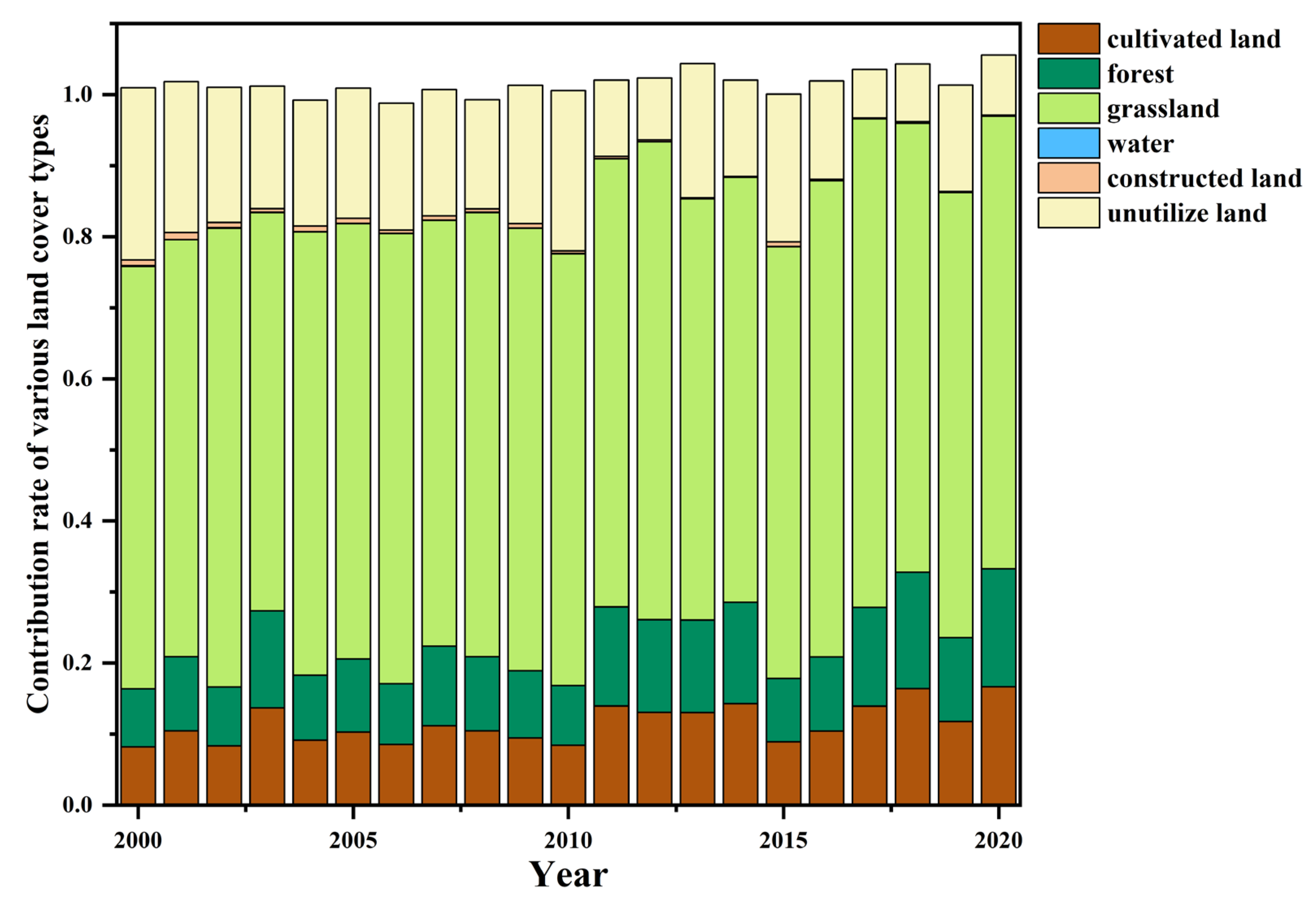
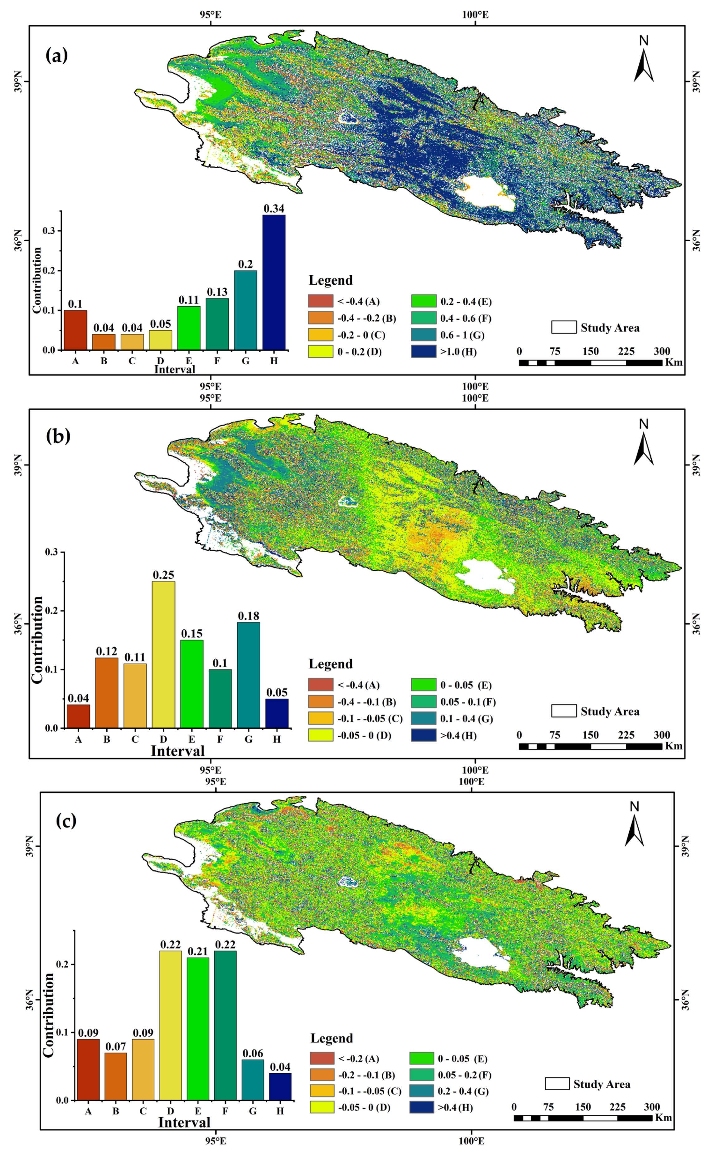

Disclaimer/Publisher’s Note: The statements, opinions and data contained in all publications are solely those of the individual author(s) and contributor(s) and not of MDPI and/or the editor(s). MDPI and/or the editor(s) disclaim responsibility for any injury to people or property resulting from any ideas, methods, instructions or products referred to in the content. |
© 2023 by the authors. Licensee MDPI, Basel, Switzerland. This article is an open access article distributed under the terms and conditions of the Creative Commons Attribution (CC BY) license (https://creativecommons.org/licenses/by/4.0/).