Spatiotemporal Variations of Aerosol Optical Depth and the Spatial Heterogeneity Relationship of Potential Factors Based on the Multi-Scale Geographically Weighted Regression Model in Chinese National-Level Urban Agglomerations

Abstract

Investigating the spatiotemporal variation characteristics of aerosol optical depth (AOD) and its driving factors is essential for assessing atmospheric environmental quality and alleviating air pollution. Based on a 22-year high-resolution AOD dataset, the spatiotemporal variations of AOD in mainland China and ten national urban agglomerations were explored based on the Mann–Kendall trend test and Theil–Sen median method. Random forest (RF) and multiscale geographically weighted regression (MGWR) were combined to identify the main driving factors of AOD in urban agglomerations and to reveal the spatial heterogeneity of influencing factors. The results showed that areas with high annual average AOD concentrations were mainly concentrated in the Chengdu–Chongqing, Central Plains, Shandong Peninsula, and Middle Yangtze River urban agglomerations. Southern Beijing–Tianjin–Hebei and its surrounding areas revealed the highest AOD pollution during summer, whereas the worst pollution during the remaining three seasons occurred in the Chengdu–Chongqing urban agglomeration. Temporally, except for the Ha-Chang and Mid-Southern Liaoning urban agglomerations, where the average annual AOD increased, the other urban agglomerations showed a decreasing trend. Among them, the Central Plains, Middle Yangtze River, Guanzhong Plain, and Yangtze River Delta urban agglomerations all exhibited a decline greater than 20%. According to the spatial trends, most urban agglomerations encompassed much larger areas of decreasing AOD values than areas of increasing AOD values, indicating that the air quality in most areas has recently improved. RF analysis revealed that PM_2.5 was the dominant factor in most urban clusters, followed by meteorological factors. MGWR results show that the influencing factors have different spatial scale effects on AOD in urban agglomerations. The socioeconomic factors and PM_2.5 showed strong spatial non-stationarity with regard to the spatial distribution of AOD. This study can provide a comprehensive understanding of AOD differences among urban agglomerations, and it has important theoretical and practical implications for improving the ecological environment and promoting sustainable development.

1. Introduction

Aerosols constitute mixed multiphase systems of very small solid or liquid particles suspended in the atmosphere along with gas carriers [1], with a scale ranging from approximately 0.001–100 μm. Aerosols can significantly impact ecology, human health [2], and physicochemical processes in the atmosphere [3], and they can influence global and regional climate patterns through direct radiative forcing and indirect effects (e.g., affecting cloud formation) [4]. Additionally, much aerosol particulate matter contributes to hazy weather, which reduces atmospheric visibility [5]. The risk to human health resulting from prolonged exposure to air with high aerosol concentrations is significant [6]. Therefore, it is crucial to comprehensively understand the properties and causes that affect the spatiotemporal distributions of aerosols. Aerosol optical depth (AOD) is an important optical property of aerosols, which mainly describes the light extinction capacity of aerosols within the whole atmospheric column, and it is an important physical parameter for measuring air pollution degree [7]. In addition, AOD is strongly correlated with the surface air quality (e.g., particulate matter with an aerodynamic diameter less than 2.5 μm (PM_2.5) and PM₁₀) [8], which is important for estimating aerosol concentrations and studying climate change characteristics. Initially, ground-based station observations were the primary sources of AOD data, but due to the sparse and uneven distribution of observation sites, it was difficult to assess the spatiotemporal distribution characteristics of aerosol particulate matter across wide continuous areas [9]. With the development of remote sensing technology, satellite remote sensing data exhibit the advantages of high continuity and broad coverage, which compensates for the shortage of ground-based station data and it provides critical data support for continuing investigations of aerosol characteristics and atmospheric pollution monitoring on large spatial and long-term time scales.

Urban agglomerations, as highly developed forms of the integrated urban space, are products of high-level national industrialization and urbanization at an advanced stage [10]. However, with the deepening of economic globalization and urbanization, many urban diseases have emerged (e.g., high greenhouse gas emissions [11], enhanced urban heat island effects [12], increased extreme heat [13], and urban ecological damage [14]). Among them, air pollution has emerged as a global environmental pollution problem [15]. The exceedance of pollutants, such as particulate matter, nitrogen dioxide, and ozone, is a major challenge in terms of improving urban air quality [16,17,18,19]. Internationally, the development of AOD inversion algorithms [20,21,22,23,24], the spatiotemporal distribution of AOD and pollution characteristics [25,26,27,28,29,30], PM_2.5 estimation, and others [31,32,33,34,35,36] have been extensively investigated. Most importantly, a thorough understanding of the spatiotemporal distribution patterns of aerosols in various regions, over long time series, and the mechanism of their effects on air pollution and climate change is essential. Gupta et al. [37] researched the AOD pollution level at eight key locations worldwide, and they discovered that the Middle East, East China, and Central China exhibited the highest AOD pollution levels.

Over the past few decades, China has experienced accelerated urbanization and industrialization, whereas Chinese cities are facing serious air pollution concerns. The spatiotemporal distribution characteristics and dynamic trends in aerosols in China have been quantitatively analyzed in many studies in recent years [38,39,40]. Some studies are limited to one or a few cities or urban clusters, such as Beijing [41], the Yangtze River Delta [42], and the Guanzhong region [9]. Scholars have also studied the entire country [38], and the findings suggest that the locations with the highest AOD pollution levels in China are primarily centered in North China, the middle reaches of the Yangtze River, Chengdu, and Chongqing. However, recent research has primarily concentrated on more developed regions, with little focus on areas such as the Central Plains and Northeast China. In several studies, the heterogeneity in the spatiotemporal distribution patterns of AOD among Chinese metropolitan agglomerations has been ignored. Therefore, it is necessary to comparatively study aerosol particulate pollution in several national urban agglomerations in China to investigate AOD differences.

The spatiotemporal distribution of AOD is the result of complex synergistic effects of multiple emission sources and various factors. Current studies have identified the main driving factors affecting AOD at different scales in China, such as meteorological factors (rainfall, relative humidity, temperature, wind speed, etc.) [7], topographic and surface factors (Digital Elevation Model (DEM), Normalized differential vegetation index (NDVI) etc.) [38], and socioeconomic factors [39,43]. Multiple linear regression [44], principal component analysis [45], the Pearson correlation coefficient, and the geographic detector method [5] are commonly used to explore the relationship between each influencing factor and AOD concentration. These methods can easily evaluate the correlation between AOD and the impact factor, but the nonlinear response relationship and spatial characteristics between AOD and impact factor are ignored. The multi-scale geographically weighted regression model (MGWR) can be improved based on the geographically weighted regression model. The multi-scale spatial effects between AOD and different variables can be taken into account using this model, which can better demonstrate the spatial non-stationarity of AOD influencing factors in different regions [46]. In addition, the random forest regression model (RF) has been increasingly applied in the research of geographical objects to quickly identify the relative importance of AOD influencing variables in different urban agglomerations, to enhance the explanatory power of the model [47]. Therefore, it is necessary to comprehensively explore the regulatory mechanisms of the numerous influencing factors of AOD and to research and analyze the variability of drivers in different urban agglomerations throughout China.

In summary, to further reveal the spatial distribution characteristics and multiple factors influencing the AOD in this study, we selected ten urban agglomerations with high urbanization and economic development levels in China based on the Multi-Angle Implementation of Atmospheric Correction (MAIAC) AOD data. The main research components in this study include the following: (1) to analyze and compare the spatial patterns and changing characteristics of AOD on multiple spatial scales; (2) to explore the trends and differences of AOD; and (3) to identify the main driving factors of AOD, and to explore the spatial heterogeneity relationship between AOD and driving factors.

2. Materials and Methods

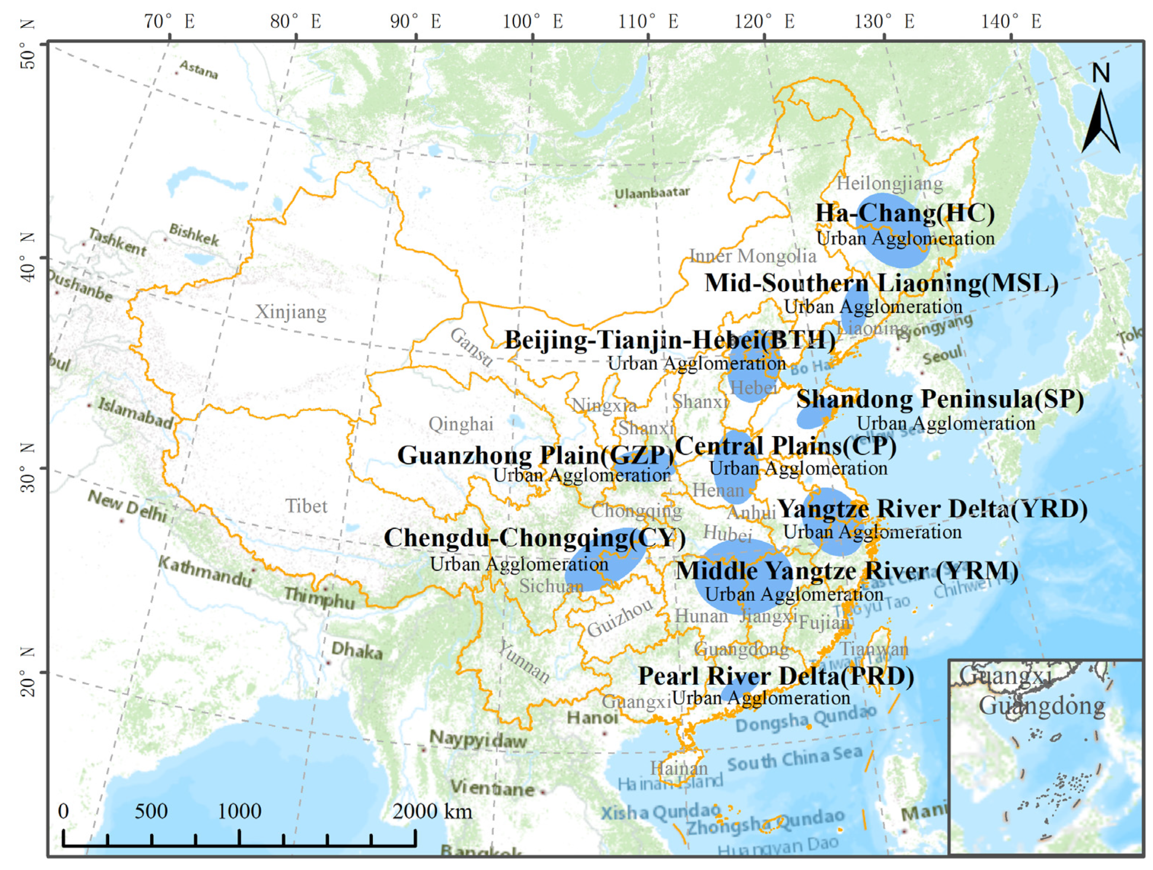
2.1. Study Areas

As shown in Figure 1, the study area mainly includes ten urban agglomerations with high urbanization and economic development levels in China. These ten urban agglomerations are as follows: the Beijing–Tianjin–Hebei (BTH), the Yangtze River Delta (YRD), the Pearl River Delta (PRD), the Middle Yangtze River (YRM), the Chengdu–Chongqing (CY), the Central Plains (CP), the Shandong Peninsula (SP), the Guanzhong Plain (GZP), the Ha-Chang (HC), and the Mid-Southern Liaoning (MSL).

BTH is the economic core of China, but is also one of China’s most polluted areas [48]. YRD is an important intersection of the One Belt–One Road area and the Yangtze River Economic Belt. It occupies a pivotal strategic position in China’s national modernization and opening pattern. PRD is the main region of China that participates in economic globalization, and it exhibits favorable air dispersion conditions, but its rapid economic development and population growth still significantly impact the air quality. YRM is an important part of the Yangtze River Economic Belt, which is a major part of the Yangtze River. CY is the most economically and culturally developed region in western China and it is a heavily polluted region in the southwest [49]. CP is the birthplace of the Chinese nation and Chinese civilization, and its urban groups are the largest and most densely populated, with a highly developed transportation network, which imposes great pressure on the ecological environment. SP is one of the more important dense urban areas in East China, it is on the outskirts of the vast hinterland of the middle and lower reaches of the Yellow River, with a high economic development level, and an area with serious air pollution. GZP is located at the center of inland China, and it is the second-largest urban agglomeration in the western region. HC and MSL are two regional urban clusters in the north, where most of China’s heavy industries are distributed, so the atmospheric environment must still be considered [50].

These urban agglomerations, which cover the majority of mainland China and include most of the typical climatic zones, are characterized by a variety of geographic conditions, climate types, surface types, and urban morphologies, as well as extensive spatial variability. It has been shown that most urban agglomerations face serious air pollution problems during urbanization and economic development, especially BTH, YRM, YRD, and CY [48,51,52]. Therefore, we chose these areas as regional-scale study objects. Details of these urban agglomerations are shown in Supplementary Table S1. It should be noted that several regions of Qinghai were excluded due to satellite observations of AOD anomalies in these regions.

2.2. Materials

2.2.1. MCD19A2

MCD19A2 data constitute the latest release of NASA’s Moderate Resolution Imaging Spectroradiometer (MODIS) AOD product C6 version, which uses the MAIAC algorithm with a spatial resolution of 1 km and a wavelength of 550 nm [53,54]. Compared with traditional algorithms, the MAIAC algorithm is a general algorithm based on image processing and time series analysis; this provides higher accuracy for dark background surfaces with green vegetation and bright background surfaces, such as desert areas [55]. The high resolution, high precision, and extensive coverage of the MAIAC AOD data products are advantageous, and their accuracy has been confirmed throughout China [56,57].

Therefore, we collected monthly AOD products covering mainland China from 2000 to 2021 using the Google Earth Engine geospatial analysis platform. Based on the GEE database, all daily AOD product data (MCD19A2) were masked by a quality control band (AOD_QA), whereas pixels containing clouds and surfaces with snow and ice were excluded; these observations were then aggregated into monthly composite data. To ensure the accuracy of the results, the peripheral 5 × 5 pixel mean values were selected to fill the missing values. Further discussions concerning the data are provided in Text S1 in the Supplementary Materials.

2.2.2. Auxiliary Data

To investigate the driving factors behind the spatiotemporal distributions of AOD, 11 influencing factors were selected, including meteorological factors, topographic factors, surface characteristic factors, socioeconomic factors, and pollution indicators. Details of these influencing factors are provided in

Table 1. Auxiliary data list.

Data Type	Data	Resolution	Data Source
Meteorological factors	Relative humidity (RH)	1000 m 1 month (Tmp and RH are the near-surface product data)	National Earth System Science Data Center, National Science and Technology Infrastructure of China (http://www.geodata.cn (accessed on 8 November 2022)) [58]
	Temperature (Tmp)
	Precipitation (Prcp)
	Wind speed (WS)
Topographic factors	Digital Elevation Model (DEM)	1000 m	Resource and Environment Science and Data Center (https://www.resdc.cn/ (accessed on 4 November 2022))
	Slope
Surface characteristics factors	Normalized differential vegetation index (NDVI)	250 m 16 d	(https://data.tpdc.ac.cn (accessed on 15 March 2023)) [59]
	Land surface temperature (LST)	1000 m 8 d	Resource and Environment Science and Data Center (https://www.resdc.cn/ (accessed on 7 April 2023))
Pollution indicator	PM2.5	1000 m	(https://weijing-rs.github.io/ (accessed on 20 February 2023)) [57]
Socioeconomic factors	Gross Domestic Product (GDP)	1000 m	Resource and Environment Science and Data Center (https://www.resdc.cn/ (accessed on 8 June 2022))
	Population Density (PD)

.

2.3. Methodology

2.3.1. Theil–Sen Median Method

The Theil–Sen Median method is a robust nonparametric statistical method for trend calculations that is computationally efficient, insensitive to outliers, and suitable for the AOD trend analysis of long time series data [60]. Its calculation formula is as follows:

$$S_{AOD}=Medain\left(\frac{{AOD}_j-{AOD}_i}{j-i}\right),2000\le i<j\le 2021$$

where ${AOD}_i$ and ${AOD}_j$, respectively, present the annual average values of AOD in years $i$ and $j$. $S_{AOD}$ denotes the trend of the AOD long time series, $S_{AOD}>0$, and $S_{AOD}<0$ is the mean of the increasing and decreasing trend of AOD.

2.3.2. Mann–Kendall Test

The Mann–Kendall (MK) trend test method is a nonparametric time series trend test method that has been extensively used in studies of climate, hydrology, and vegetation greenness changes. It is suitable for the significance testing of consistent trends that increase or decrease in long-time series data [61]. Therefore, the MK trend test method was chosen to determine the trend in AOD dynamics; the trend test is performed using the test statistic Z. The Z value is calculated as follows:

$$\mathrm{Z}=\left\{\begin{array}{c}\frac{S-1}{\sqrt{Var\left(S\right)}},S>0\\ 0,\\ \frac{S-1}{\sqrt{Var\left(S\right)}},S<0\end{array}\right.$$

where: $Var\left(S\right)=\frac{n(n-1)(2n+5)}{18}$, $S={\sum }_{i=1}^{n-1}{\sum }_{j=i+1}^{n}sgn\left({AOD}_j-{AOD}_i\right),$

$$sgn\left({AOD}_j-{AOD}_i\right)=\left\{\begin{array}{c}1,{AOD}_j-{AOD}_i>0\\ 0,{AOD}_j-{AOD}_i\le 0\end{array}\right.$$

where n is the number of time series and $\mathrm{s}\mathrm{g}\mathrm{n}\left(\right)$ is the symbolic function. $Z>0$ and $Z<0$ denote the increasing and decreasing trends of AOD, respectively. When the absolute value of Z is greater than 1.65, 1.96, and 2.58, the trend is considered to pass the significance test of 90%, 95%, and 99%, respectively.

Combined with the application of the MK trend test method and the Theil–Sen median trend analysis method, the annual trends regarding AOD changes in China, from 2000–2021, were determined using the MATLAB 2020 platform with the annual AOD data of China.

2.3.3. Random Forest (RF) Regression Model

The random forest (RF) algorithm is based on a bagging integrated learning approach [62]. It is a classifier that uses multiple trees to train and predict samples. Classification, regression, and other problems can be solved. The RF model can quickly explore the complex relationships between multiple factors, and it can quantitatively assess the contribution of the influencing factors. Currently, the RF model has been widely used for research in biology [63], medicine, geography [64], and other fields. Therefore, RF regression models were employed to identify the main drivers of the spatiotemporal distribution of AOD in the ten urban agglomerations, and to obtain the relative importance based on the contribution rate.

Using the R Studio platform, samples from each of the 10 urban agglomerations were stratified and sampled using the randomForest software package. For internal model validation (out-of-bag (OOB) error), 70% of the samples were randomly selected as training samples, and 30% of the samples were used as test samples. The optimal parameters of the RF regression model were finally determined by adjusting the number of decision trees and the number of evaluations per node to reduce the OOB error. In RF classification models, ntree is the number of base classifiers included, which is set to 100, and mtry is the number of variables included in each decision tree, which is set to 5. To estimate the importance of the influencing factors, a percentage increase in the mean squared error (%IncMSE) of the variables was adopted. A higher %IncMSE value indicates a greater contribution of the variable and a higher importance ranking. The rfPermute software package was used to measure the significance of each variable’s contribution to AOD [65]. Finally, bar charts demonstrating the relative importance of the drivers of AOD in each urban agglomeration were generated using software packages such as ggplot2.

2.3.4. Multi-Scale Geographically Weighted Regression (MGWR)

The multi-scale geographically weighted regression model (MGWR) is an essential tool for spatial heterogeneity analysis. This method not only compensates for the spatial variability among variables, which is ignored by typical regression analysis methods, but it also optimizes the independent bandwidth of each variable. It is an optimization improvement to the geographically weighted regression model, which ensures that the results are closer to reality [66]. When performing the coefficients of distinct independent variables, the spatial distribution heterogeneity scales concerning the differences of the respective variables are taken into account by MGWR, and multiple spatial scales and kernel functions are applied to the data. Therefore, MGWR is utilized to estimate the spatial heterogeneity relationship between AOD and meteorological, socioeconomic, surface, and pollution indicators in urban agglomerations. The calculation formula is as follows [67]:

$$y_i=\sum _{\mathrm{j}-1}^{\mathrm{k}}{\beta }_{bwj}\left(u_i,v_i\right)x_{ij}+{\epsilon }_i$$

where $y_i$ is AOD; $bwj$ is the bandwidth used by the regression coefficient of the $j$; $\left(u_i,v_i\right)$ denotes the spatial geographic coordinates of $i$; ${\beta }_{bwj}$ is the position corresponding to the regression coefficient of the $j$ variable; $x_{ij}$ is the value of the $\mathrm{j}\mathrm{t}\mathrm{h}$ independent variable at position $i$; and ${\epsilon }_i$ is the error term of the model at position i.

The MGWR model used in this study was constructed based on the MGWR 2.2 software developed by Oshan et al. [68], where the adaptive bi-square was chosen as the kernel function for the calculation of the weight matrix, and a corrected Akaike information criterion (AICc) was used as the criterion for determining the optimal bandwidth. The 22-year annual mean AOD of urban agglomerations was used as the dependent variable, and the influence factors were used as the independent variables to further explore the spatial non-stationarity of the influence of different factors on AOD.

3. Results

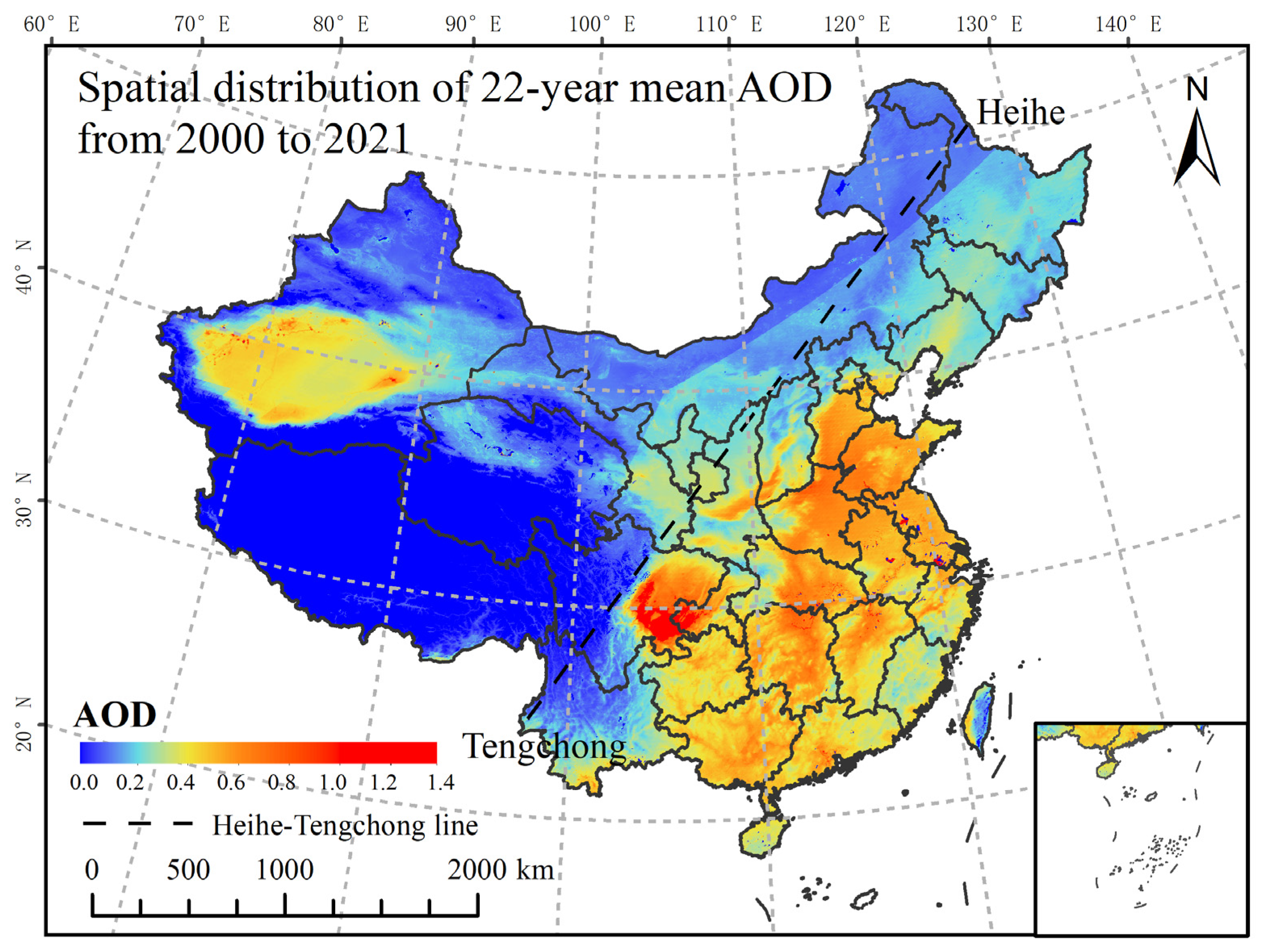
3.1. Spatial Pattern of AOD

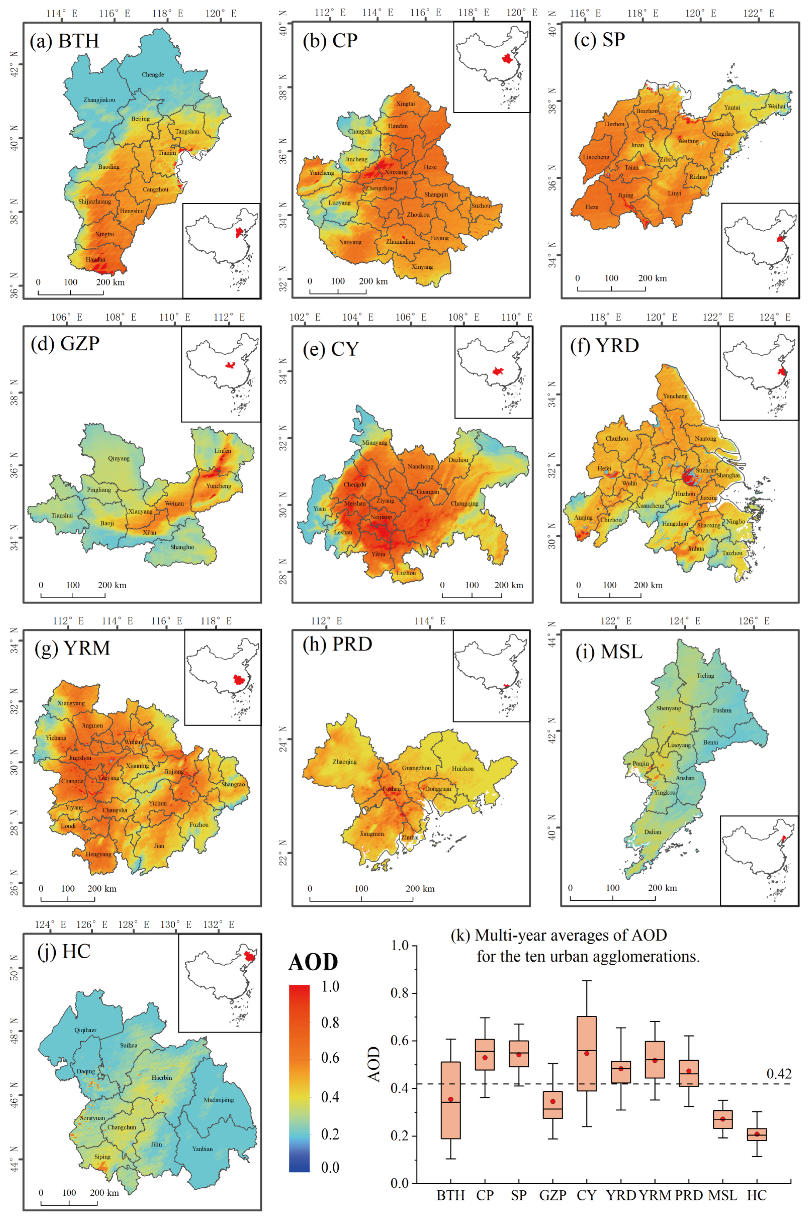
3.1.1. Spatial Distribution of Annual AOD in Ten Urban Agglomerations

From 2000 to 2021, the multi-year average AOD value across China was 0.27. Figure 2 shows the 22-year average annual spatial distribution pattern of AOD in China. In terms of spatial distribution, high AOD values were primarily concentrated in densely populated areas (eastern China), east of the Heihe–Tengchong line, such as the North China Plain, the middle reaches of the Yangtze River, and the Sichuan Basin, whereas low AOD values generally occurred in areas west of the Heihe–Tengchong line (western China), which is consistent with previous studies [38,69,70]. Additionally, the southwestern part of the Xinjiang Autonomous Region (i.e., the Taklamakan Desert), is the center of pollution in western China. The presence of large deserts and basins, sparse vegetation, and a combination of arid climate conditions have resulted in frequent sandy and dusty weather events and high AOD levels in this region [71]. AOD decreased in most of China from 2000 to 2021, whereas the spatial distribution of AOD has remained consistent, and most of eastern China (Sichuan Basin, North China Plain, and Central China Plain, etc.) is still an area that comprises high AOD concentrations (Supplementary Figure S1).

The spatial distribution of AOD in the different urban agglomerations exhibited regional variability and spatial heterogeneity. The spatial distribution of AOD in urban agglomerations generally decreased in CY, CP, and YRM to the surrounding area, and HC and MSL in the northeast region had the lowest AOD. Figure 3a–j shows the spatial distribution of the 22-year AOD mean values of urban agglomerations, and Figure 3k shows the box plot of the abovementioned AOD values. The 22-year AOD average of all urban agglomerations was calculated to be 0.42 (

Table 2. Variations in annual average AOD concentrations and the rate of change (R) (%) for China and urban agglomerations.

	2000–2021	R2021–2000	2000	2005	2010	2015	2021
China	0.27	−8.3	0.24	0.26	0.28	0.27	0.22
M-UA	0.42	−11.9	0.38	0.44	0.45	0.44	0.32
BTH	0.36	−9.1	0.33	0.34	0.36	0.38	0.30
CP	0.53	−27.5	0.51	0.54	0.53	0.57	0.37
SP	0.54	−10.6	0.47	0.54	0.60	0.60	0.42
GZP	0.35	−25	0.36	0.37	0.34	0.36	0.27
CY	0.54	−17.0	0.47	0.62	0.69	0.47	0.39
YRD	0.47	−25	0.44	0.49	0.47	0.48	0.33
YRM	0.52	−25	0.44	0.57	0.54	0.52	0.33
PRD	0.47	−3.0	0.34	0.56	0.50	0.42	0.32
MSL	0.27	4.4	0.23	0.26	0.24	0.32	0.24
HC	0.21	18.8	0.16	0.16	0.18	0.24	0.19

M-UA represents the mean AOD of all urban agglomerations. R was calculated as (a − b)/b × 100%. Where a is 2021, b is 2000.

). To better understand the AOD level of urban agglomerations, 0.3, 0.42, and 0.5 were selected as threshold values, according to Figure 3k and Table 2. There are four categories of AOD values.

The first category of high-value urban agglomerations (AOD > 0.5) included CY, SP, CP, and YRM. The Sichuan Basin is the center of high AOD values for CY, and it exhibited a gradual decrease in all directions (Figure 3e). The Sichuan Basin experiences a humid climate and is surrounded by mountains, facilitating the formation of a thermal inversion layer, which impedes aerosol particle diffusion, thus leading to a higher aerosol load in CY [72]. Cities within CP and SP generally have high AOD (Figure 3b,c). This phenomenon may be related to the dense population, traffic congestion, and the high proportion of the coal industry. The high AOD values in the city cluster in YRM are distributed in a ring shape, and they decrease from north to east (Figure 3g). The second category of sub-high-value urban agglomerations (0.42 < AOD < 0.5) included YRD and PRD. YRD features an advanced water system (Figure 3f). Influenced by lakes and rivers, the warm and humid climate is conducive to aerosol concentration in the atmosphere [42]. PRD exhibited high AOD values, mainly in central areas such as Guangzhou and Foshan (Figure 3h), because high urban economic development level and intensive human activities take place in these regions [73]. The AOD of the third category of sub-low-value urban agglomerations (0.3 < AOD < 0.42) indicated significant regional variability. BTH encompasses Xingtai as the center of high values, and the AOD value gradually decreased in the north (Figure 3a). The AOD high-value areas in GZP were distributed in a stepped pattern (Figure 3g) that was mainly influenced by the topography and mountain ranges [74]. HC and MSL are low-value urban agglomerations (AOD < 0.3) that exhibit the lowest aerosol loads and the lowest spatial heterogeneity regarding AOD (Figure 3i,j). However, Northeast China is an area wherein industrial and heavy industrial activities are concentrated, and to a significant extent, the high AOD values coincide with the industrial geographical distribution. In addition, industrial soot emissions, wastewater, waste gas originating from chemical raw materials and manufacturing, and extensive biomass burning reduce atmospheric quality [75].

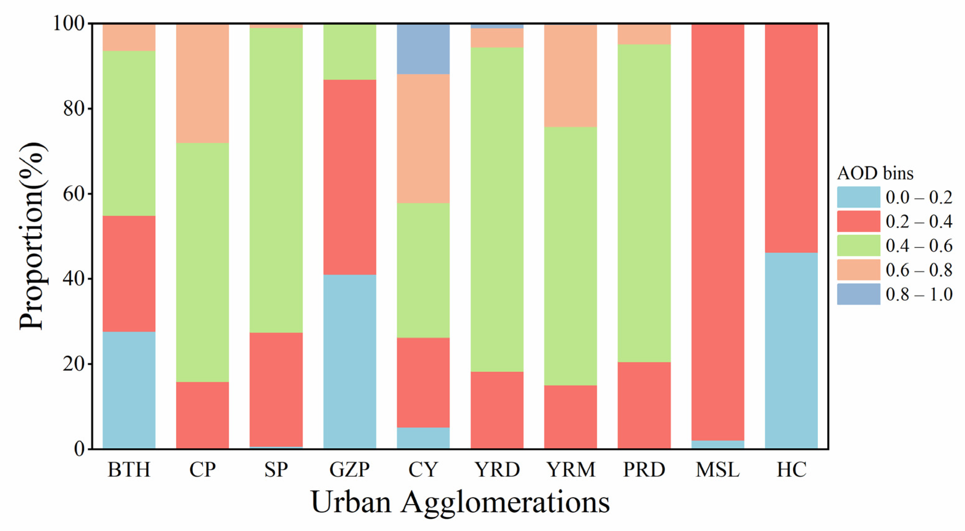
3.1.2. Frequency Distribution of Annual AOD in Ten Urban Agglomerations

As shown in Figure 4, in order to understand the distribution of the 22-year AOD concentrations in different value intervals, we analyzed the frequency of the occurrence of various AOD levels in ten urban agglomerations in units of 0.2. The highest frequency of extreme clean conditions (AOD < 0.2) was found in HC (~46%), followed by GZP (~41%). The frequency of 0.2 < AOD < 0.4 was highest in MSL (98%), then HC, GZP (50%), and the remaining urban clusters (20%, evenly distributed). With the increase in AOD, the frequency of 0.4 < AOD < 0.6 was observed in more than 56% of CP, SP, YRD, YRM, and PRD. At the 0.6 < AOD < 0.8 level, AOD dropped to less than 30% in many urban agglomerations, and less than 1% in SP and GZP. CY emerged with a frequency of about 12% at 0.8 < AOD < 1.0, and it appeared almost infrequently in other urban agglomerations. These results indicated that HC, MSL, and GZP had the highest frequencies in the range of 0.2 < AOD < 0.4, and 0.4 < AOD < 0.6, for the other urban groups. There was a tendency for AOD frequency to decrease with increasing AOD.

Additionally, we discovered that there is a relationship between the level of frequency of AOD occurrence in different urban agglomerations and the geographical distance between them. CP and YRM are neighbors, both contain only three AOD frequency ranges, and they have similar proportions. Both BTH and GZP exhibited comparable levels in terms of the frequency of occurrence of AOD and AOD values. The similar frequency of AOD occurrence implied that marine-type aerosols might be an important component of AOD in SP, YRD, and PRD. Although the level of AOD composition in MSL and HC was similar, HC was found more frequently at 0 < AOD < 0.2, which indicated that its internal urban air quality was cleaner. Notably, CY had the most AOD frequency components, covering a range of AOD values that included a variety of ranges, which indicated that CY’s inner-city aerosol particulate matter was composed of a more diverse mix of particulate matter of multiple particle sizes.

3.2. Temporal Variability of AOD

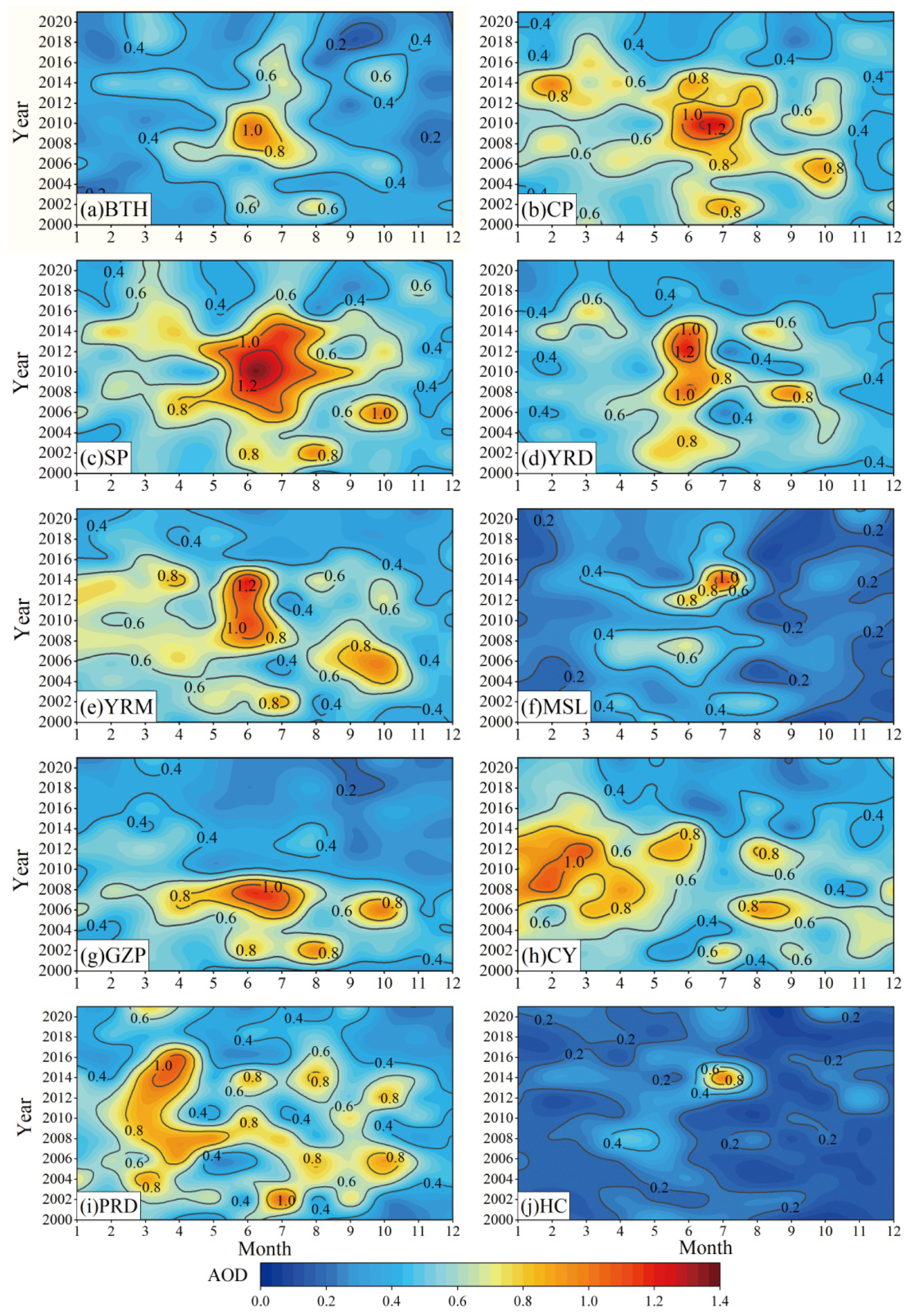
3.2.1. Annual and Monthly Variations in the Urban Agglomerations

The average monthly change in AOD in each of the ten urban agglomerations for 2000–2021 is shown in Figure 5. During the study period, the centers with high AOD values in the 10 urban agglomerations differed, and the values gradually decreased over time. The AOD high-value centers for BTH, CP, SP, YRM, YRD, and MSL were mainly concentrated in June or July 2012–2014 (Figure 5a–f). The monthly average concentrations in SP were higher than those in the other five urban agglomerations. High aerosol loads were concentrated in June and July of 2010, with a maximum value of 1.38, which is higher than the AOD values in the other urban agglomerations during the same period. This may occur because SP experiences a humid summer climate and it contains a coastline on three sides, which promotes aerosol accumulation. Additionally, the dense urban distribution, heavy traffic, industrial structure, and biomass burning produce particulate emissions, which increase aerosol loads [76]. The variations in AOD_MAS (the monthly average AOD values) in CP, YRD, and YRM were also roughly similar to those found for SP. CP reached its maximum AOD value (1.27) around June 2010, whereas the maximum AOD values in YRD and YRM emerged in June 2012 and 2014, respectively; for both YRD and YRM, the value was 1.21. AOD_MAS in BTH and MSL were relatively low. The highest AOD in BTH was 1.02 in June 2010, whereas the highest AOD in MSL (1.09) occurred in July 2014. In general, AOD_MA (the monthly average AOD value) in MSL was lower than that in the other urban agglomerations. The aerosol load values were still high even though AOD_MAS in these six urban agglomerations dramatically dropped over time.

The distribution patterns of AOD_MAS in GZP, CY, PRD, and HC are different (Figure 5g–j). From 2000–2010, the monthly mean maximum value of AOD in GZP occurred in the summer and reached its highest point (1.14) in June 2008. After 2010, AOD peaked (0.56) in February or March. The primary causes for this may be the low vegetation cover in spring, the Loess Plateau in Northwest China, and the activity of cold air masses which can lead to sandstorms or even dust storms; this increased the particulate matter concentration and particles were transported to the Guanzhong region [74]. The 22-year AOD average value in CY was the highest, and AOD_MA peaked in February and November (Figure 5h). The AOD_MAS in CY remained stable between 2000 and 2003. Between 2004 and 2014, the AOD_MA reached a maximum in February and March, with a maximum value of 1.07. After 2015, there was a decline each month. There were multiple centers of variation in AOD_MAS in PRD. From 2000 to 2012, the high AOD values in this urban agglomeration were mainly concentrated in March, April, July, and October. After 2012, the high AOD values decreased, and the high values tended to be concentrated in March of each year, with a maximum value of 1.06. This phenomenon may be caused by the large number of industrial regions in the hinterland of PRD, the rapid urbanization, and the high particulate emissions [77]. On the other hand, PRD in March was dominated by rainy weather, so the increase in aerosol hygroscopic growth intensified the extinction effect of solar incident radiation in the atmosphere. At the same time, given the dominance of southerly winds, coastal industrial particulate emissions, and sea salt blowing inland, an increase in the total amount of particulate matter was found in the atmosphere [73]. Compared with other urban agglomerations, the AOD_MAS in HC were generally lower. The highest monthly average AOD value (0.98) was reached in July 2014. A possible reason for this is that the moisture absorption of particulate matter increases due to the abundant rain in the summer of HC, which leads to an increase in AOD. On the other hand, in densely populated and industrially developed urban areas, the anthropogenic emissions of aerosol particles are lifted to the upper layers by urban heat [75]. Overall, HC exhibited high AOD values in winter. This is primarily caused by the high number of particulate matter emissions into the atmosphere in the northeast as a result of centralized heating. In addition, the number of fire points is much greater than in other provinces, and particulate matter resulting from straw burning and the formation of secondary aerosols all aggravate local and regional air pollution levels [75].

In general, although the changes in the AOD_MA in the different urban agglomerations exhibited different characteristics, there has been a reduction in AOD in recent years. The majority of locations have improved air quality, and the reduction in the aerosol load suggests that air pollution management policies have made some progress. However, many urban agglomerations with dense populations and growing economic development (e.g., CP and YRM) still exhibit high AOD load levels, thus necessitating continued attention to air pollution problems.

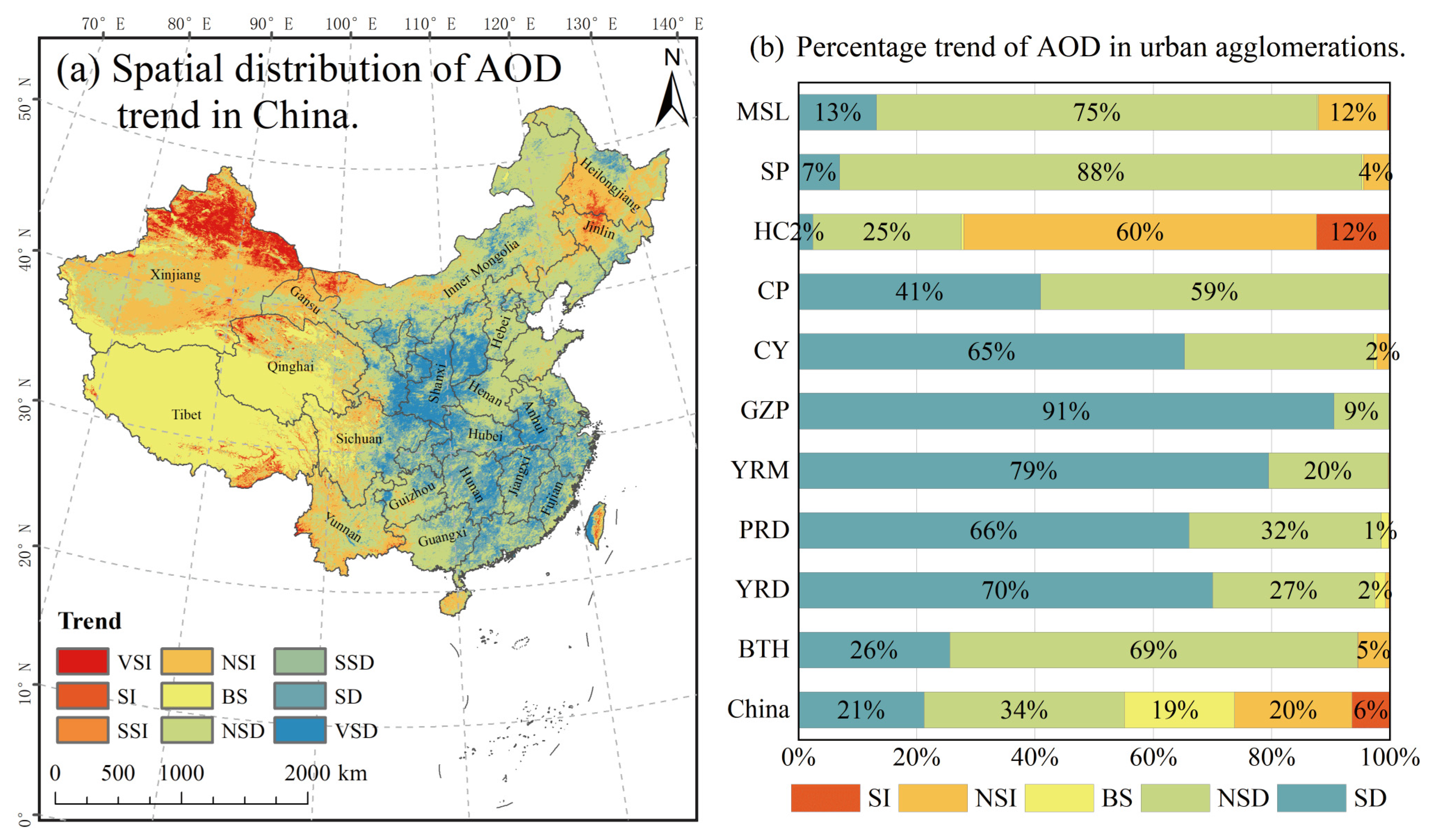
3.2.2. Trends in the Annual Average AOD for 2000–2021

Based on the MK trend test and Theil–Sen median trend analysis results, the changing trends, regarding AOD in China, were categorized into nine groups (

Table 3. AOD trend and its percentage change in China.

${\mathit{S}}_{\mathit{A}\mathit{O}\mathit{D}}$	Z	Trend Categories	Trend Feature	Percentage Change of AOD in China
$S_{AOD}>0$	2.58 < Z	4	Very significantly increased (VSI)	6.42%
	1.96 < Z ≤ 2.58	3	Significantly increased (SI)
	1.65 < Z ≤ 1.96	2	Slightly significantly increased (SSI)
	Z ≤ 1.65	1	Nonsignificantly increased (NSI)	19.85%
$S_{AOD}=0$	Z	0	Basically stable (BS)	18.64%
$S_{AOD}<0$	Z ≤ 1.65	−1	Nonsignificantly decreased (NSD)	33.89%
	1.65 < Z ≤ 1.96	−2	Slightly significantly decreased (SSD)	21.20%
	1.96 <Z ≤ 2.58	−3	Significantly decreased (SD)
	Z < 2.58	−4	Very significantly decreased (VSD)

${\mathrm{S}}_{AOD}$ denotes the trend of AOD long time series, Z denotes the trend test.

), and the spatial distribution of each category is shown in Figure 6a. The AOD changing trends were further divided into five major categories based on the AOD trend change analysis results, as follows: significantly decreased (SD), nonsignificantly decreased (NSD), basically stable (BS), nonsignificantly increased (NSI), and significantly increased (SI). In China, AOD exhibited a decreasing trend in 55.09% of the regions, and a significant increasing trend was found in 6.42% of the regions (Table 3). Among them, the regions with a significantly decreasing trend in terms of AOD were concentrated in Shaanxi Province, southern Shanxi Province, southeastern Anhui Province, etc. The regions with a significantly increasing trend regarding AOD were mainly distributed in northern Xinjiang, which may occur because this region is in the economic belt area along the northern slope of Tianshan Mountain, and it is the most economically developed region in Xinjiang. Moreover, this region borders the Taklamakan Desert, Junggar Basin, and Turpan Basin, all of which are affected by dusty weather conditions and exhibit a significantly increasing trend in terms og aerosol concentration, which is consistent with the findings of the study [78].

From the perspective of urban agglomerations, the change in AOD in the ten urban agglomerations showed a significant decrease from northeast to southwest. As shown in Figure 6b, apart from HC, the area of significant decline was much larger than the areas that significantly increased in the other urban agglomerations, including YRD, PRD, YRM, GZP, CY, and CP. The percentages of the areas that exhibited a significant reduction were 70%, 66.02%, 79.47%, 90.54%, 65.29%, and 40.91%, respectively, demonstrating China’s success in preventing and reducing air pollution. However, as these areas are still important areas for intensive human activities and socioeconomic development, air pollution prevention and control measures still cannot be ignored. In contrast, the area (12.4%) with a significantly increasing AOD tendency was larger than the HC area (2.39%), which exhibited a significant decreasing AOD trend. The significant increase in AOD was mainly concentrated in the Changchun–Jilin industrial belt and the Harbin–Daqing–Qiqihar industrial belt. Due to the interactions between human activities, widespread industrial belts, and weather patterns, these areas may exhibit an increasing trend [50]. Overall, the urban agglomerations in southeastern China, GZP, and CY in the west were locations where aerosol concentrations rapidly decreased, whereas the particulate matter concentrations of AOD in the northeast increased.

3.3. Analysis of the Importance of Factors Affecting AOD in Urban Agglomerations Based on the Random Forest Algorithm

To obtain a comprehensive understanding of the primary drivers of AOD changes in the 10 urban agglomerations from 2000 to 2021, the contribution of 11 drivers to AOD (%IncMSE) was evaluated using the RF method, and they were ranked in terms of their relative importance (Figure 7). The findings indicated that each driver imposed an independent effect on the AOD in the urban clusters with varying contribution rates. PM_2.5 is one of the most important influencing variables with regard to the change in AOD, with a contribution rate to the YRM AOD being as high as 24.82%. The contribution rate of PM_2.5 was not only highest in CP, SP, GZP, YRD, and MSL, but it also significantly differed from that of the secondary factors, at 6.94%, 6.15%, 3.81%, 4.82%, and 5.80%, respectively. Meteorological factors also greatly contributed to AOD, with Tmp contributing the most to AOD in PRD (16.04%), and RH to AODs in HC (16.76%) and CY (17.38%). Concerning each urban agglomeration, WS contributed the least, particularly in YRD, with a contribution of only 2.15% that failed the significance test. The remaining six driving factors all influenced the AOD in urban agglomerations to varying degrees. For example, DEM contributed more to AODs in CP (15.18%), SP (15.43%), and YRM (16.02%); LST contributed the most to YRM (17.98%); and GDP ranked in the top three in YRD and YRM, and it yielded the highest contribution rate (18.85%). Overall, the components, sources, and changes in AOD were not dominated by a single factor, but were the result of the combined effects of pollution indices, meteorological factors, topographic conditions, and socioeconomic factors. Climate, geographic location, human activities, intra-urban spatial organization, and function should all be considered for the various urban agglomerations and locations.

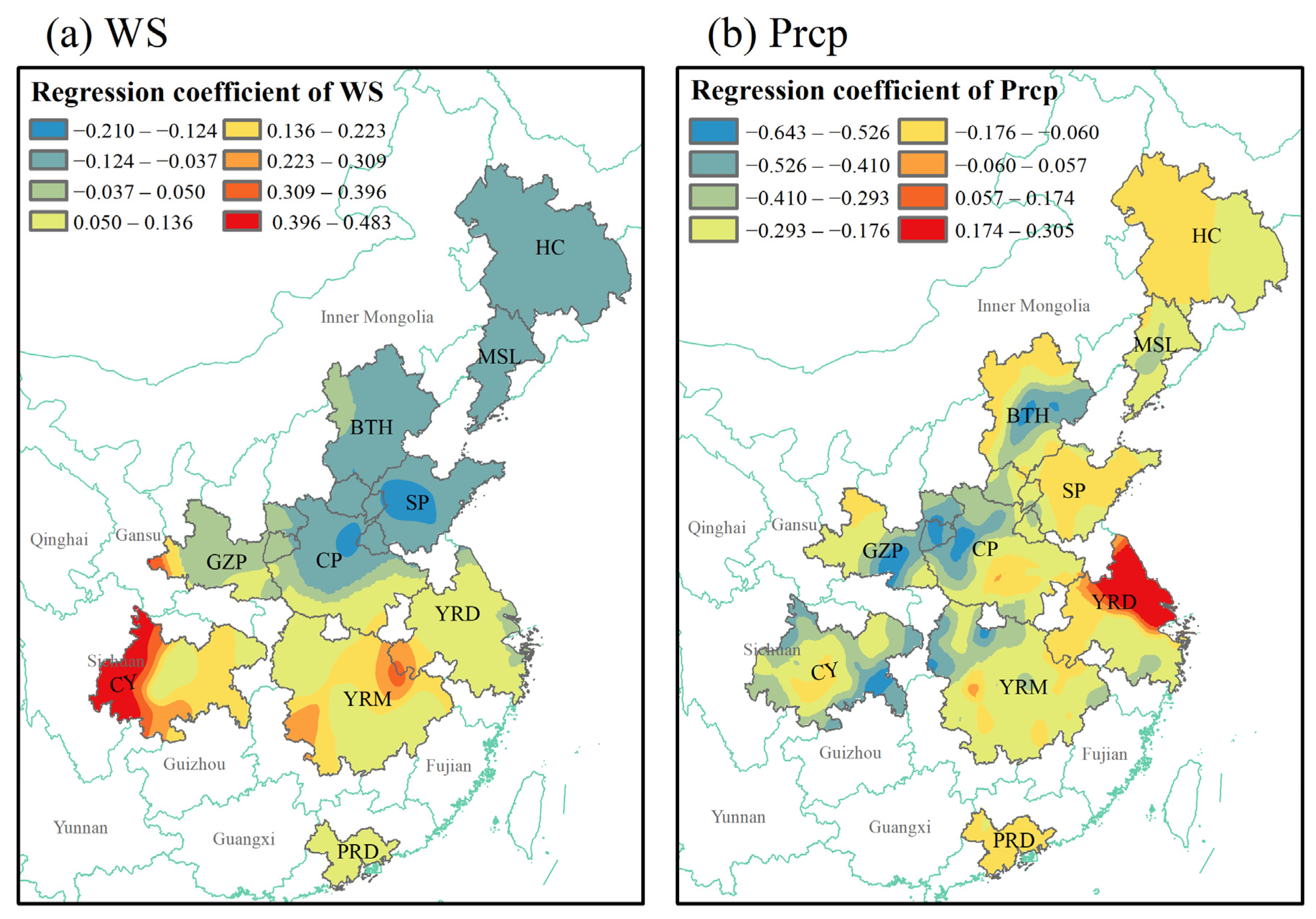
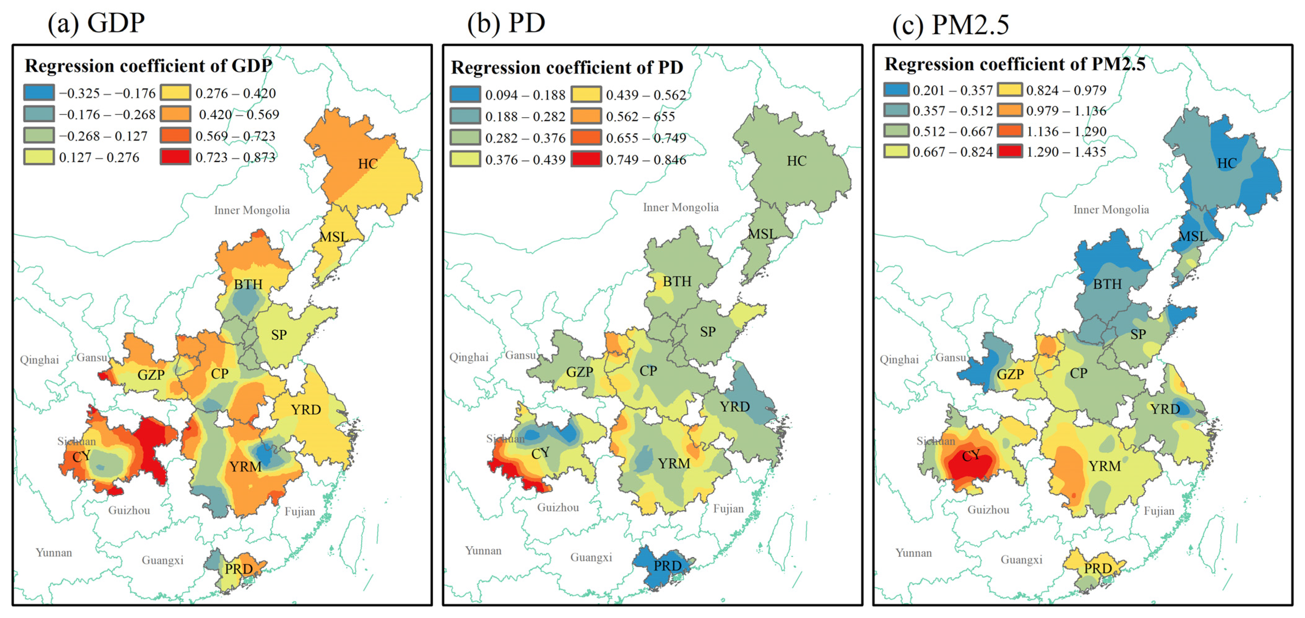
3.4. Spatial Heterogeneity of AOD and Influencing Factors in Urban Agglomerations

The MGWR model not only revealed the direction and intensity of the influence of each factor on AOD, but it also demonstrated the spatial heterogeneity of the response of each factor with AOD using statistically significant drivers. Note that multicollinearity between the variables can distort the results of the assessment of spatial heterogeneity [66,79]. Therefore, using the local linear test, variables with a variance inflation factor (VIF) of <5 were retained (Supplementary Table S2), including eight variables (i.e., PM2.5, DEM, Slope, GDP, PD, NDVI, WS, and RH). All parameters were estimated to be statistically significant with p values < 0.05. Figure 8, Figure 9 and Figure 10 show the spatial heterogeneity of responses to AOD for each factor.

The regression coefficient of meteorological factors is shown in Figure 8. The intensity of WS influence on the urban agglomerations’ AOD ranges from −0.210 to 0.483, and Prcp ranges from −0.643 to 0.305. Both of their influences on the AOD were bidirectional. The spatial influence of WS on AOD roughly decreased from southwest to northeast (Figure 8a). Negative impacts mainly occurred in the urban agglomerations north of the central CP, but their intensity was low (0.037–0.210). The AOD was positively impacted by WS in urban agglomerations south of the central part of CP, with the strong positive impacts concentrated in the western regions of CY and at the intersection of YRM and YRD. The spatial influence of Prcp on AOD in urban agglomerations was more fragmented (Figure 8b). Strong positive correlations were mainly concentrated in the northeastern part of YRD, whereas strong negative correlations were discretely distributed within some city clusters (e.g., the east–central part of BTH, the neighboring cities of CP and GZP, and the southeastern part of CY).

The regression coefficients of the terrain surface factor are shown in Figure 9. The area of negative influence, regarding DEM on AOD, was larger than the area of positive influence, with regression coefficients ranging from −1.081 to 0.260 (Figure 9a). The strong negative impact was mainly concentrated in the center of CY, whereas the areas with an intense positive impact occurred in the northwestern part of HC. The influence of Slope on the AOD of the urban agglomerations was negative (Figure 9b). The strong negative impact mainly appeared in the western region of the CP, whereas the intensity of the negative influence in the area east of the CP was relatively weak (0.037–0.124). The negative effect of NDVI and AOD was mainly observed in PRD, YRM, HC, CY, SP, and some parts of BTH (Figure 9c); this indicates that vegetation in these locations provided favorable conditions for the reduction of aerosol particles [4]. Although NDVI produced positive effects for AOD in GZP and CP, perhaps because the urban and built-up areas encompass a vast area, vegetation affects the urban airflow, reducing the dispersion of pollutants, and human-induced aerosol particles aggregate more in these areas [80]. In contrast to other influencing factors, however, the overall intensity of the effect of NDVI on AOD in urban agglomerations was weak (−0.121 to 0.101).

The regression coefficients of the socioeconomic factors and pollution indicator are shown in Figure 10. The direction of the effect of GDP on AOD is bi-directional, with regression coefficients ranging from −0.325 to 0.873 (Figure 10a). The areas where GDP has a positive influence on AOD are larger than areas where it has a negative influence on AOD, and the strong positive impact is concentrated in the eastern part of the CY (0.723 to 0.873). The positive effect of PD on AOD in the urban agglomeration was significant (0.094–0.846), with a strong positive effect concentrated in the southwestern part of the CY (Figure 10b). The regression coefficients for the pollution indicator, PM2.5, ranged from 0.201 to 1.435, which showed a strong positive correlation (Figure 10c). The overall spatial distribution of the influence of PM2.5 on AOD shows a gradual increase from northeast to southwest. The intensity of impacts is greatest in south-central CY (1.290–1.435), and lowest in HC, MSL, and BTH. These results suggest that the southern urban agglomerations (especially CY), with their rapid economic development, complex industrial structure, and relatively high concentration of population density, are highly polluted areas in terms of particulate matter pollution.

4. Discussion

4.1. Drivers and Potential Mechanisms of AOD in Ten Urban Agglomerations

4.1.1. Multi-Scale Relationship between Impact Factors and AOD in Urban Agglomerations

Compared with the global model results (GLR) (adjusted R² is 0.740 and AICc is 7319.516), the MGWR model’s adjusted R² is 0.983, and the AICc is −5315.893. Higher adjusted R² and lower AICc values imply a higher performance. The MGWR model results indicated that the influence factors have different spatial scale effects on AOD in urban agglomerations (Supplementary Figure S2). The spatial bandwidth of the surface factors was observed to be more stable compared with other factors from 2000–2021. Prcp, GDP, PD, and Slope have the widest spatial bandwidths, indicating that these factors are global variables with similar spatial effects on the AOD of different urban agglomerations. The spatial bandwidths of WS, DEM, NDVI, and PM2.5 are minimal, indicating that these effects are local variables with AOD spatial changes in different places.

4.1.2. The Influence of AOD Concentration Management in Different Urban Agglomerations

As shown in Figure 3k, the spatial distribution pattern of AOD in ten urban agglomerations is divided into two parts. GZP, BTH, MSL, and HC have lower AODs, whereas the high values of AOD are distributed in the six urban agglomerations south of East China. This spatial distribution is closely related to the influencing factors. The mechanisms of aerosol particulate matter diffusion, transfer, and deposition are significantly influenced by meteorological variables. This study demonstrates that the meteorological factors show great differences in terms of contribution, intensity, and direction of AOD in different urban agglomerations. Among all the impact factors, RH contributed the most to the AOD of CY and HC, and Tmp contributed the most to PRD. WS can have important effects on the propagation and dispersion of near-surface aerosols. On the one hand, WS could reduce aerosol concentration; for instance, if there existed a negative correlation between WS and AOD in SP, it indicates that the higher the wind speed in these areas, the easier aerosol diffusion occurs. On the other hand, wind speed transports pollutants across some places, increasing the amount of aerosol particles. For instance, WS was significantly and positively correlated with the AOD in CY, showing that winds can transport a large amount of particulate matter, which reduces air quality [7]. The effect of Prcp on AOD in different urban agglomerations is complex. Prcp has a negative impact on AOD in BTH, CP, and most areas of GZP. This may be because the higher humidity promotes the formation of rainfall. The washing effect of the rain will contribute to the deposition of particulate matter, resulting in a reduction in the concentration of aerosol pollution [81]. On the contrary, Prcp shows a strong positive influence in the southeastern part of YRD. It indicated that when the air humidity is high in the coastal area of YRD, particulate matter is prone to hygroscopic expansion, which, in turn, undergoes secondary transformation to form aerosols.

According to studies, population distribution can be influenced by topographic and geomorphic features, which can then indirectly affect the spatial distribution of AOD [38,82,83]. The population density is significantly higher where there is a strong link between DEM and AOD (e.g., CP, CY), which leads to an increase in anthropogenic aerosol emissions and more severe air pollution. In addition, surface factors and their evolution are the most intuitive performance characteristics of regional and urban development, which are also directly related to the sources of pollution emissions and the locations where pollutants are deposited [83]. Under various levels of economic development, urban building intensity, and population distribution, the mechanisms of pollution generation, accumulation, and diffusion vary substantially. The AOD values are generally lower in areas with higher urban green space and vegetation cover. In contrast, AOD values are generally higher in urban clusters with higher surface temperatures (e.g., CY, CP, etc.). In regions with faster urbanization, anthropogenic aerosols generated via anthropogenic activities such as traffic exhaust emissions, construction dust, biomass combustion, and home heating account for a particularly large proportion of urban aerosols [84], and thus, AOD is more significantly affected by human activities. These findings imply that topographic and geomorphic factors and socioeconomic elements have a specific synergistic relationship. Moreover, the urban spatial pattern and surface characteristics of different urban agglomerations may change the regional meteorological conditions, air convection characteristics, etc., which, in turn, regulate the accumulation and diffusion of atmospheric aerosols in different regions, thus leading to variability in the spatial distribution of AOD in urban agglomerations.

4.2. Relationship between AOD Concentration and Environmental Policy Implementation

The change in AOD in the ten urban agglomerations from 2000–2021 is roughly consistent with AOD in China (Supplementary Figure S3). This phenomenon may be related to the various economic development strategies and environmental policies promulgated and implemented by the Chinese government.

From 2000 to 2010, China’s regions made great efforts to develop their economies, and the urbanization level continued to rise. According to the Tenth Five Year Plan (2001–2005), China’s economic and social development will be particularly significant over the next five to ten years [85]. Moreover, there has been an increase in industrial waste, vehicle emissions, and construction dust, resulting in rising particulate matter concentrations and hazy weather. Between 2003 and 2008, China experienced its worst air pollution events. Notably, 2008 was an important turning point in terms of air pollution control [86]. In the run-up to the Beijing Olympic Games, a series of air pollution prevention and control measures were adopted by governments across China to slow the increase of particulate matter levels in order to meet international air quality standards. Among these measures, the Beijing Olympic Games Air Quality Assurance Program proposed air management and emission reduction measures for BTH. In terms of emission reduction, particulate emissions in Beijing have been significantly reduced, and the surrounding areas have applied changes to the industrial structure of critical regions, such as the elimination of obsolete oil-fired boilers and steel production processes [87]. Although air pollution has been alleviated in most areas, AOD in various urban agglomerations remains high, and air pollution concerns continue to plague most Chinese cities.

From 2011–2021, many urban agglomerations were still developing their economies, and there was a slight rebound in AOD concentrations, resulting in persistant air problems. To effectively control air pollution, the State Council promulgated the National Environmental Protection 12th Five-Year Plan in 2012, and the Air Pollution Prevention and Control Action Plan in 2013, which set out strict pollution control measures. Beginning in 2014, the reduction rate of pollutants in China was significantly accelerated [88], and aerosol particulate matter concentrations significantly decreased. Among them, CY experienced an accelerated reduction rate of its AOD concentrations in 2013. This was due to the Sichuan provincial government’s air pollution prevention and control program for CY, which proposed various measures, such as the strict control of new pollutant emissions, the optimization of the energy structure, and the implementation of the synergistic control of multiple pollutants [89]. In addition, the State Council officially issued the Three-Year Action Plan for Winning the Blue Sky Defense War in 2018, which continues to guide the implementation of air pollution prevention and control actions in the three key areas of BTH and surrounding areas, YRD, and the Fenwei Plain [90]. Local governments have responded to the action plan by introducing corresponding measures. For example, Shandong Province amended its air pollution prevention and control regulations in 2018, stating that the focus is on preventing and controlling coal pollution, as well as industrial and related forms of pollution, dust pollution, agricultural pollution, and other types of pollution, which has led to a continuous decline in AOD values [76].

Generally, as the Chinese government executes various pollution control measures, air quality issues in China and the ten urban agglomerations will gradually be resolved. However, there is obvious spatial and temporal variability in terms of AOD in the ten urban agglomerations, and many cities are still comprise high AOD values; for example, the Sichuan Basin in CY, Handan in southern BTH, and Jiaozuo and Puyang in CP. Chinese urban agglomerations still face tremendous challenges in aerosol air pollution management, and relevant environmental protection departments should still focus on polluted areas and develop appropriate regional air pollution control strategies in the future.

4.3. Uncertainties and Limitations

There are uncertainties and limitations in this study that should be further considered and improved. First, the eleven drivers were selected based on the available data. Among them, only GDP and PD were considered as socioeconomic factors. In future studies, factors such as city size, built-up areas, urban industrial structures, and industrial points of interest (POIs) in different urban agglomerations should be studied in depth as important influencing factors. Second, this study only revealed the relative importance and spatial heterogeneity of the influencing factors for the spatiotemporal distributions of 22-year AOD average values. Future research should focus on examining the relationship between AOD and influencing factors using various time scales (e.g., annual, seasonal, and monthly scales) to comprehensively understand the mechanism of AOD drivers, and to provide evidence to support the development of air pollution control measures.

5. Conclusions

In this study, the spatiotemporal variations of AOD from 2000 to 2021 were examined using annual and monthly time scales, considering ten Chinese urban agglomerations with favorable circumstances for economic development and urbanization. The quantitative model for the correlation between AOD and potential factors was established using the RF and MGWR methods to identify the key influencing factors and spatial heterogeneity of AOD in the various urban agglomerations.

The results demonstrated that between 2000 and 2021, high AOD values were mainly concentrated in eastern China. The annual average AOD values in the urban agglomerations exhibited regional variation and spatial heterogeneity, and the annual average AOD changes showed an initial upward trend and a subsequent downward trend. Regarding the monthly time scale, the centers of the average monthly variation in AOD differed among the ten urban agglomerations. The monthly AOD averages in BTH, CP, SP, YRM, YRD, and MSL reached their maximum values in June or July each year. Spatial change trend analysis revealed that AOD in 12.4% of HC showed a significant upward trend, whereas AOD’s downward trend in the remaining urban agglomerations was greater than the upward trend. The analysis of the spatiotemporal variation of AOD showed that the air quality of the ten urban agglomerations was gradually improving. However, the annual average AOD values in most urban agglomerations were greater than 0.3 in 2021, which indicates that the AOD pollution situation in most areas remains severe.

According to the RF method, the main drivers of AOD changes with regard to urban agglomerations significantly differed. PM_2.5 was closely related to AOD, and it was the main driver in BTH, CP, SP, GZP, YRD, YRM, and MSL. RH was the main driver in CY and HC, whereas Tmp was the primary driver in PRD. The MGWR model reveals the spatial heterogeneity of factors and the AOD of urban agglomerations in terms of influence, intensity, and spatial pattern, which provides more spatial details. The results of the MGWR model show that the influencing factors have different spatial scale effects on the AOD of urban agglomerations. Compared with other factors, the spatial bandwidth of the surface factor is more stable. The effects of WS, Prcp, DEM, NDVI, and GDP on the AOD of the ten urban agglomerations are bi-directional, whereas PM2.5 and PD have a positive effect on the AOD, and Slope has a negative effect. These results imply that there is a complex coupling between meteorological factors, socioeconomics, surface topography, and other factors. Therefore, aerosols and the relevant departments of the urban agglomerations should consider the impacts of different drivers on AOD to formulate reasonable and scientific atmospheric prevention and control measures.

References

1. Liu, Y.; Lin, A.; QIin, W.; He, L.; Li, X. Spatial-Temporal Distribution of Aerosol Optical Depth and Its Main Influence Types in China during 1990–2017. Environ. Sci. 2019, 40, 2572–2581. [Google Scholar] [CrossRef]
2. Cai, H.; Yang, Y.; Luo, W.; Chen, Q. City-level variations in aerosol optical properties and aerosol type identification derived from long-term MODIS/Aqua observations in the Sichuan Basin, China. Urban Clim. 2021, 38, 100886. [Google Scholar] [CrossRef]
3. Chen, Q.-X.; Huang, C.-L.; Yuan, Y.; Mao, Q.-J.; Tan, H.-P. Spatiotemporal Distribution of Major Aerosol Types over China Based on MODIS Products between 2008 and 2017. Atmosphere 2020, 11, 703. [Google Scholar] [CrossRef]
4. Niu, L.; Wang, X.; Han, H.; Liang, X.; Jiang, X.; Tan, Z.; Liu, Z. Spatiotemporal distribution of aerosol optical depth in the five Central Asian countries. Acta Sci. Circumstantiae 2021, 41, 321–333. [Google Scholar] [CrossRef]
5. Cheng, L.; Li, L.; Chen, L.; Hu, S.; Yuan, L.; Liu, Y.; Cui, Y.; Zhang, T. Spatiotemporal Variability and Influencing Factors of Aerosol Optical Depth over the Pan Yangtze River Delta during the 2014–2017 Period. Int. J. Environ. Res. Public Health 2019, 16, 3522. [Google Scholar] [CrossRef]
6. Ping, S.; Runhua, W.; Gao, C.; Rongshu, Z. Research progress on heterogeneous oxidation of organic tracers of atmospheric aerosols. Environ. Chem. 2023, 42, 1–11. [Google Scholar]
7. Deng, X.; Shi, C.; Wu, B.; Chen, Z.; Nie, S.; He, D.; Zhang, H. Analysis of aerosol characteristics and their relationships with meteorological parameters over Anhui province in China. Atmos. Res. 2012, 109–110, 52–63. [Google Scholar] [CrossRef]
8. Su, Q.; Li, J.; Chen, M. A review of satellite remote sensing inversion studies of atmospheric aerosols. Sci. Technol. Innov. Her. 2019, 16, 108–112. [Google Scholar] [CrossRef]
9. Yang, X.; Wang, X.; Cui, S.; Feng, Z.; Jiang, Z. Spatio-temporal Distribution Characteristics and Influencing Factors of Different Aerosol Types in the Guanzhong Area. Acta Sci. Circumstantiae 2023, 43, 343–352. [Google Scholar] [CrossRef]
10. Shen, Z.; Xu, X.; Sun, Z.; Jiang, Y.; Shi, H. Regional thermal environments (RTEs) and driving forces in six urban agglomerations of China and America. Build. Environ. 2023, 235, 110185. [Google Scholar] [CrossRef]
11. Liu, X.; Huang, Y.; Xu, X.; Li, X.; Li, X.; Ciais, P.; Lin, P.; Gong, K.; Ziegler, A.D.; Chen, A.; et al. High-spatiotemporal-resolution mapping of global urban change from 1985 to 2015. Nat. Sustain. 2020, 3, 564–570. [Google Scholar] [CrossRef]
12. Wang, Z.; Meng, Q.; Allam, M.; Hu, D.; Zhang, L.; Menenti, M. Environmental and anthropogenic drivers of surface urban heat island intensity: A case-study in the Yangtze River Delta, China. Ecol. Indic. 2021, 128, 107845. [Google Scholar] [CrossRef]
13. Wu, S.; Wang, P.; Tong, X.; Tian, H.; Zhao, Y.; Luo, M. Urbanization-driven increases in summertime compound heat extremes across China. Sci. Total Environ. 2021, 799, 149166. [Google Scholar] [CrossRef]
14. Peng, J.; Ma, J.; Liu, Q.; Liu, Y.; Hu, Y.; Li, Y.; Yue, Y. Spatial-temporal change of land surface temperature across 285 cities in China: An urban-rural contrast perspective. Sci. Total Environ. 2018, 635, 487–497. [Google Scholar] [CrossRef] [PubMed]
15. Zhao, X.; Zhou, W.; Han, L.; Locke, D. Spatiotemporal variation in PM(2.5) concentrations and their relationship with socioeconomic factors in China’s major cities. Environ. Int. 2019, 133, 105145. [Google Scholar] [CrossRef]
16. Li, Z.; Bai, L.; Feng, J.; Liu, S.; Duan, C.; Zhang, Y. Characteristics of aerosol optical depth dynamics and their causes over typical cities along the 21st Century Maritime Silk Road. Chin. J. Appl. Ecol. 2021, 32, 2565–2577. [Google Scholar] [CrossRef]
17. Kumar, A.; Ambade, B.; Sankar, T.K.; Sethi, S.S.; Kurwadkar, S. Source identification and health risk assessment of atmospheric PM2.5-bound polycyclic aromatic hydrocarbons in Jamshedpur, India. Sustain. Cities Soc. 2020, 52, 101801. [Google Scholar] [CrossRef]
18. Ambade, B.; Sankar, T.K.; Sahu, L.K.; Dumka, U.C. Understanding Sources and Composition of Black Carbon and PM2.5 in Urban Environments in East India. Urban Sci. 2022, 6, 60. [Google Scholar] [CrossRef]
19. Ambade, B. Characterization of PM10 over urban and rural sites of Rajnandgaon, central India. Nat. Hazards 2015, 80, 589–604. [Google Scholar] [CrossRef]
20. Yan, X.; Li, Z.; Luo, N.; Shi, W.; Zhao, W.; Yang, X.; Liang, C.; Zhang, F.; Cribb, M. An improved algorithm for retrieving the fine-mode fraction of aerosol optical thickness. Part 2: Application and validation in Asia. Remote Sens. Environ. 2019, 222, 90–103. [Google Scholar] [CrossRef]
21. Sun, L.; Sun, C.; Liu, Q.; Zhong, B. Aerosol optical depth retrieval by HJ-1/CCD supported by MODIS surface reflectance data. Sci. China Earth Sci. 2011, 53, 74–80. [Google Scholar] [CrossRef]
22. Merdji, A.B.; Xu, X.; Lu, C.; Habtemicheal, B.A.; Li, J. Accuracy assessment and climatology of MODIS aerosol optical properties over North Africa. Environ. Sci. Pollut. Res. 2022, 30, 13449–13468. [Google Scholar] [CrossRef] [PubMed]
23. Giles, D.M.; Sinyuk, A.; Sorokin, M.G.; Schafer, J.S.; Smirnov, A.; Slutsker, I.; Eck, T.F.; Holben, B.N.; Lewis, J.R.; Campbell, J.R.; et al. Advancements in the Aerosol Robotic Network (AERONET) Version 3 database–automated near-real-time quality control algorithm with improved cloud screening for Sun photometer aerosol optical depth (AOD) measurements. Atmos. Meas. Tech. 2019, 12, 169–209. [Google Scholar] [CrossRef]
24. Li, R.; Sun, L.; YU, H.; Wei, J.; Tian, X. An Improved DDV Algorithm for the Retrieval of Aerosol Optical Depth from NOAA/AVHRR Data. J. Indian Soc. Remote Sens. 2021, 49, 1141–1152. [Google Scholar] [CrossRef]
25. Abuelgasim, A.; Bilal, M.; Alfaki, I.A. Spatiotemporal variations and long term trends analysis of aerosol optical depth over the United Arab Emirates. Remote Sens. Appl. Soc. Environ. 2021, 23, 100532. [Google Scholar] [CrossRef]
26. Musonda, B.; Jing, Y.; Nyasulu, M.; Libanda, B. Long-term spatial and temporal variations of aerosol optical depth during 2000–2020 over Zambia, southcentral Africa. Air Qual. Atmos. Health 2021, 15, 177–193. [Google Scholar] [CrossRef]
27. Dadashi-Roudbari, A.; Ahmadi, M. Evaluating temporal and spatial variability and trend of aerosol optical depth (550 nm) over Iran using data from MODIS on board the Terra and Aqua satellites. Arab. J. Geosci. 2020, 13, 277. [Google Scholar] [CrossRef]
28. Payra, S.; Gupta, P.; Bhatla, R.; El Amraoui, L.; Verma, S. Temporal and spatial variability in aerosol optical depth (550 nm) over four major cities of India using data from MODIS onboard the Terra and Aqua satellites. Arab. J. Geosci. 2021, 14, 1256. [Google Scholar] [CrossRef]
29. Kumar, P.; Kapur, S.; Choudhary, A.; Singh, A.K. Spatiotemporal variability of optical properties of aerosols over the Indo-Gangetic Plain during 2011–2015. Indian J. Phys. 2021, 96, 329–341. [Google Scholar] [CrossRef]
30. Kim, H.-S.; Chung, Y.-S.; Kim, J.-T. Spatio-temporal variations of optical properties of aerosols in East Asia measured by MODIS and relation to the ground-based mass concentrations observed in central Korea during 2001∼2010. Asia-Pac. J. Atmos. Sci. 2013, 50, 191–200. [Google Scholar] [CrossRef]
31. Carmichael, G.R.; Adhikary, B.; Kulkarni, S.; D’Allura, A.; Tang, Y.; Streets, D.; Zhang, Q.; Bond, T.C.; Ramanathan, V.; Jamroensan, A.; et al. Asian Aerosols: Current and Year 2030 Distributions and Implications to Human Health and Regional Climate Change. Environ. Sci. Technol. 2009, 43, 5811–5817. [Google Scholar] [CrossRef]
32. Kim, S.-M.; Koo, J.-H.; Lee, H.; Mok, J.; Choi, M.; Go, S.; Lee, S.; Cho, Y.; Hong, J.; Seo, S.; et al. Comparison of PM2.5 in Seoul, Korea Estimated from the Various Ground-Based and Satellite AOD. Appl. Sci. 2021, 11, 10755. [Google Scholar] [CrossRef]
33. Zang, Z.; Li, D.; Guo, Y.; Shi, W.; Yan, X. Superior PM2.5 Estimation by Integrating Aerosol Fine Mode Data from the Himawari-8 Satellite in Deep and Classical Machine Learning Models. Remote Sens. 2021, 13, 2779. [Google Scholar] [CrossRef]
34. Han, M.; Jia, S.; Zhang, C. Estimation of high-resolution PM2.5 concentrations based on gap-filling aerosol optical depth using gradient boosting model. Air Qual. Atmos. Health 2022, 15, 619–631. [Google Scholar] [CrossRef]
35. Chen, Q.-X.; Huang, C.-L.; Yuan, Y.; Mao, Q.-J.; Tan, H.-P. Assessment of aerosol types on improving the estimation of surface PM2.5 concentrations by using ground-based aerosol optical depth dataset. Atmos. Pollut. Res. 2019, 10, 1843–1851. [Google Scholar] [CrossRef]
36. Lu, J.; Zhang, Y.; Chen, M.; Wang, L.; Zhao, S.; Pu, X.; Chen, X. Estimation of monthly 1 km resolution PM2.5 concentrations using a random forest model over “2 + 26” cities, China. Urban Clim. 2021, 35, 100734. [Google Scholar] [CrossRef]
37. Gupta, G.; Venkat Ratnam, M.; Madhavan, B.L.; Jayaraman, A. Global trends in the aerosol optical, physical, and morphological properties obtained using multi-sensor measurements. Atmos. Environ. 2023, 295, 119569. [Google Scholar] [CrossRef]
38. He, Q.; Gu, Y.; Zhang, M. Spatiotemporal patterns of aerosol optical depth throughout China from 2003 to 2016. Sci. Total Environ. 2019, 653, 23–35. [Google Scholar] [CrossRef]
39. Ding, S.; He, J.; Liu, D.; Zhang, R.; Yu, S. The spatially heterogeneous response of aerosol properties to anthropogenic activities and meteorology changes in China during 1980–2018 based on the singular value decomposition method. Sci. Total Environ. 2020, 724, 138135. [Google Scholar] [CrossRef]
40. Liu, Z.; Shi, C.; Zhang, M.; Gao, Z.; Zhu, X.; Wang, X. Temporal Characteristics of Aerosol Optical Depth Based on Cluster Analysis Method. J. Atmos. Environ. Opt. 2019, 14, 411–418. [Google Scholar]
41. Yuting, L.; Mingquan, W.; Zheng, N.; Wenjiang, H. Trend analysis of Ground-based aerosol optical thickness in Beijing from 2005 to 2018. Remote Sens. Inf. 2022, 37, 73–79. [Google Scholar]
42. Chen, Y.; Wang, J.; Chen, W.; Ma, X.; Hu, X. Spatial and temporal changes of aerosol in Yangtze river delta and its meteorological interpretation. Environ. Eng. 2021, 39, 120–127. [Google Scholar] [CrossRef]
43. Sun, K.; Chen, X.; Wang, J.; Zhang, T.; Zhu, Z. Investigation of air quality over the largest city in central China using high resolution satellite derived aerosol optical depth data. Atmos. Pollut. Res. 2018, 9, 584–593. [Google Scholar] [CrossRef]
44. He, Q.; Zhang, M.; Huang, B. Spatio-temporal variation and impact factors analysis of satellite-based aerosol optical depth over China from 2002 to 2015. Atmos. Environ. 2016, 129, 79–90. [Google Scholar] [CrossRef]
45. Zheng, Y.; Wang, X.; Zhang, X.; Hu, G. Multi-spatiotemporal patterns of aerosol optical depth and influencing factors during 2000–2020 from two spatial perspectives: The entire Yellow River Basin region and its urban agglomerations. Int. J. Appl. Earth Obs. Geoinf. 2022, 106, 102643. [Google Scholar] [CrossRef]
46. Zhou, L.; Wu, T.; Pu, L.; Meadows, M.; Jiang, G.; Zhang, J.; Xie, X. Spatially heterogeneous relationships of PM2.5 concentrations with natural and land use factors in the Niger River Watershed, West Africa. J. Clean. Prod. 2023, 394, 136406. [Google Scholar] [CrossRef]
47. Zhong, Y.; Lin, A.; Xiao, C.; Zhou, Z. Research on the Spatio-Temporal Dynamic Evolution Characteristics and Influencing Factors of Electrical Power Consumption in Three Urban Agglomerations of Yangtze River Economic Belt, China Based on DMSP/OLS Night Light Data. Remote Sens. 2021, 13, 1150. [Google Scholar] [CrossRef]
48. Shen, Y.; Zhang, L.; Fang, X.; Ji, H.; Li, X.; Zhao, Z. Spatiotemporal patterns of recent PM(2.5) concentrations over typical urban agglomerations in China. Sci. Total Environ. 2019, 655, 13–26. [Google Scholar] [CrossRef] [PubMed]
49. Xu, Y.; Guo, Z.; Zheng, Z.; Dai, Q.; Zhao, C.; Huang, W. Spatio-temporal Variation and Multi-dimensional Detection of Driving Mechanism of PM 2.5 Concentration in the Chengdu-Chongqing Urban Agglomeration from 2000 to 2021. Environ. Sci. 2022, 44, 3724–3737. [Google Scholar] [CrossRef]
50. Wang, Y.; Sun, Y.; Zhang, Z.; Cheng, Y. Spatiotemporal variation and source analysis of air pollutants in the Harbin-Changchun (HC) region of China during 2014–2020. Environ. Sci. Ecotechnol. 2021, 8, 100126. [Google Scholar] [CrossRef]
51. Zhang, L.; Zhang, M.; Yao, Y. Multi-Time Scale Analysis of Regional Aerosol Optical Depth Changes in National-Level Urban Agglomerations in China Using Modis Collection 6.1 Datasets from 2001 to 2017. Remote Sens. 2019, 11, 201. [Google Scholar] [CrossRef]
52. Tang, Y.; Xu, R.; Meng, F. Spatiotemporal evolution and prediction of AOD in typical urban agglomerations in eastern China. J. Atmos. Environ. Opt. 2021, 16, 320–330. [Google Scholar]
53. Lyapustin, A.; Wang, Y.; Korkin, S.; Huang, D. MODIS Collection 6 MAIAC algorithm. Atmos. Meas. Tech. 2018, 11, 5741–5765. [Google Scholar] [CrossRef]
54. Chudnovsky, A.A.; Kostinski, A.; Lyapustin, A.; Koutrakis, P. Spatial scales of pollution from variable resolution satellite imaging. Environ. Pollut. 2013, 172, 131–138. [Google Scholar] [CrossRef] [PubMed]
55. Lyapustin, A.I.; Wang, Y.; Laszlo, I.; Hilker, T.; Hall, F.G.; Sellers, P.J.; Tucker, C.J.; Korkin, S.V. Multi-angle implementation of atmospheric correction for MODIS (MAIAC): 3. Atmospheric correction. Remote Sens. Environ. 2012, 127, 385–393. [Google Scholar] [CrossRef]
56. Wei, J.; Huang, W.; Li, Z.; Xue, W.; Peng, Y.; Sun, L.; Cribb, M. Estimating 1-km-resolution PM2.5 concentrations across China using the space-time random forest approach. Remote Sens. Environ. 2019, 231, 111221. [Google Scholar] [CrossRef]
57. Wei, J.; Li, Z.; Lyapustin, A.; Sun, L.; Peng, Y.; Xue, W.; Su, T.; Cribb, M. Reconstructing 1-km-resolution high-quality PM2.5 data records from 2000 to 2018 in China: Spatiotemporal variations and policy implications. Remote Sens. Environ. 2021, 252, 112136. [Google Scholar] [CrossRef]
58. Jing, W.L.; Yang, Y.P.; Yue, X.F.; Zhao, X.D. A Spatial Downscaling Algorithm for Satellite-Based Precipitation over the Tibetan Plateau Based on NDVI, DEM, and Land Surface Temperature. Remote Sens. 2016, 8, 655. [Google Scholar] [CrossRef]
59. Gao, J.; Shi, Y.; Zhang, H.; Chen, X.; Zhang, W.; Shen, W.; Xiao, T.; Zhang, Y. China Regional 250 m Normalized Difference Vegetation Index Data Set (2000–2022). [Datasets]. 2023. Available online: https://data.tpdc.ac.cn/en/data/10535b0b-8502-4465-bc53-78bcf24387b3 (accessed on 25 July 2023).
60. Morell, O.; Fried, R. On Nonparametric Tests for Trend Detection in Seasonal Time Series. In Statistical Inference, Econometric Analysis and Matrix Algebra: Festschrift in Honour of Götz Trenkler; Schipp, B., Kräer, W., Eds.; Physica-Verlag HD: Heidelberg, Germany, 2009; pp. 19–39. [Google Scholar]
61. Geary, R.C. Rank Correlation Methods. Econ. J. 1949, 59, 575–577. [Google Scholar] [CrossRef]
62. Breiman, L. Random Forests. Mach. Learn. 2001, 45, 5–32. [Google Scholar] [CrossRef]
63. Yao, Y.; Liu, Y.; Zhou, S.; Song, J.; Fu, B. Soil moisture determines the recovery time of ecosystems from drought. Glob. Chang. Biol. 2023, 29, 3562–3574. [Google Scholar] [CrossRef]
64. Liu, M.; Liu, J.; Atzberger, C.; Jiang, Y.; Ma, M.; Wang, X. Zanthoxylum bungeanum Maxim mapping with multi-temporal Sentinel-2 images: The importance of different features and consistency of results. ISPRS J. Photogramm. Remote Sens. 2021, 174, 68–86. [Google Scholar] [CrossRef]
65. Jiao, S.; Chen, W.; Wang, J.; Du, N.; Li, Q.; Wei, G. Soil microbiomes with distinct assemblies through vertical soil profiles drive the cycling of multiple nutrients in reforested ecosystems. Microbiome 2018, 6, 146. [Google Scholar] [CrossRef]
66. Xue, C.; Chen, X.; Xue, L.; Zhang, H.; Chen, J.; Li, D. Modeling the spatially heterogeneous relationships between tradeoffs and synergies among ecosystem services and potential drivers considering geographic scale in Bairin Left Banner, China. Sci. Total Environ. 2023, 855, 158834. [Google Scholar] [CrossRef] [PubMed]
67. Fotheringham, A.S.; Yang, W.; Kang, W. Multiscale Geographically Weighted Regression (MGWR). Ann. Am. Assoc. Geogr. 2017, 107, 1247–1265. [Google Scholar] [CrossRef]
68. Oshan, T.; Li, Z.; Kang, W.; Wolf, L.; Fotheringham, A. mgwr: A Python Implementation of Multiscale Geographically Weighted Regression for Investigating Process Spatial Heterogeneity and Scale. ISPRS Int. J. Geo-Inf. 2019, 8, 269. [Google Scholar] [CrossRef]
69. Qian, J.; Liu, C. Distributions and changes of aerosol optical depth on both sides of HU Huanyong Line and the response to land use and land cover. Acta Sci. Circumstantiae 2018, 38, 752–760. [Google Scholar] [CrossRef]
70. Sun, Z.; Cheng, X.; Xia, X. Spatial-temporal distribution and impact factors of aerosol optical depth over China. China Environ. Sci. 2021, 41, 4466–4475. [Google Scholar] [CrossRef]
71. Feng, Y.; Chen, D.; Zhang, X. Atmospheric aerosol pollution across China: A spatiotemporal analysis of satellite-based aerosol optical depth during 2000–2016. Int. J. Digit. Earth 2018, 12, 843–857. [Google Scholar] [CrossRef]
72. Wang, A.; Kang, P.; Zhang, Y.; Zeng, S.; Zhang, X.; Shi, J.; Liu, Z.; Xiang, W.; Wang, K.; Zhang, S.; et al. Spatial differentiation and driving factors of aerosol optical depth in Sichuan Basin from 2003 to 2018. China Environ. Sci. 2022, 42, 528–538. [Google Scholar] [CrossRef]
73. He, M.; Xiao, J.; Shi, Y.; Wu, Y. Spatio-temporal distribution characteristics of aerosol optical depth in Guandong, Hong Kong and Macao from 2010 to 2019. J. Trop. Meteorol. 2021, 37, 647–655. [Google Scholar] [CrossRef]
74. Zheng, Y.; Wang, X.; Zhang, X.; Hu, G.; Liang, X.; Niu, L.; Han, H. Spatiotemporal distribution of aerosol optical depth based on Landsat data in the hinterland of the Guanzhong Basin and its relationship with urbanization. Environ. Sci. 2021, 42, 2699–2712. [Google Scholar] [CrossRef]
75. Han, Y.; Kang, L.; Song, Y. Spatial-temporal distribution of aerosol optical depth over northeastern China during 2000–2019. Acta Sci. Nat. Univ. Pekin. 2021, 57, 1027–1034. [Google Scholar] [CrossRef]
76. Wang, P.; Tang, Q.; Liang, T.; Yu, Q.; Li, X. Spatiotemporal variation of AOD in Shandong Province in recent ten years based on MODIS data. China Environ. Sci. 2021, 41, 5019–5026. [Google Scholar] [CrossRef]
77. Deng, X.; Gao, F.; Liao, S.; Liu, Y.; Chen, W. Spatiotemporal evolution patterns of urban heat island and its relationship with urbanization in Guangdong-Hong Kong-Macao greater bay area of China from 2000 to 2020. Ecol. Indic. 2023, 146, 109817. [Google Scholar] [CrossRef]
78. Yu, Z.; Li, X.; Yu, X.; Zheng, Y.; Ayitken, M.; Li, S.; Wang, N. Spatiotemporal variation characteristics of aerosol optical depth in Xinjiang from 2003 to 2019. Arid. Land. Geogr. 2022, 45, 346–358. [Google Scholar]
79. Du, H.; Zhan, W.; Voogt, J.; Bechtel, B.; Chakraborty, T.C.; Liu, Z.; Hu, L.; Wang, Z.; Li, J.; Fu, P.; et al. Contrasting Trends and Drivers of Global Surface and Canopy Urban Heat Islands. Geophys. Res. Lett. 2023, 50, e2023GL104661. [Google Scholar] [CrossRef]
80. Yang, J.; Yu, Q.; Gong, P. Quantifying air pollution removal by green roofs in Chicago. Atmos. Environ. 2008, 42, 7266–7273. [Google Scholar] [CrossRef]
81. Che, H.; Gui, K.; Xia, X.; Wang, Y.; Holben, B.N.; Goloub, P.; Cuevas-Agulló, E.; Wang, H.; Zheng, Y.; Zhao, H.; et al. Large contribution of meteorological factors to inter-decadal changes in regional aerosol optical depth. Atmos. Chem. Phys. 2019, 19, 10497–10523. [Google Scholar] [CrossRef]
82. Wang, C.; Wang, C.; Myint, S.W.; Wang, Z.H. Landscape determinants of spatio-temporal patterns of aerosol optical depth in the two most polluted metropolitans in the United States. Sci. Total Environ. 2017, 609, 1556–1565. [Google Scholar] [CrossRef]
83. Yurong, Z. Spatiotemporal Patterns of Aerosol Optical Depth and Its Influencing Factors throughout Guanzhong Region. Master’s Thesis, Northwest University, Xi’an, China, 2022. [Google Scholar]
84. Cao, C.; Lee, X.; Liu, S.; Schultz, N.; Xiao, W.; Zhang, M.; Zhao, L. Urban heat islands in China enhanced by haze pollution. Nat. Commun. 2016, 7, 12509. [Google Scholar] [CrossRef] [PubMed]
85. PRC, C.P.s.G.o.t. Outline of the Tenth Five-Year Plan for National Economic and Social Development of the People’s Republic of China. Available online: https://www.gov.cn/gongbao/content/2001/content_60699.htm (accessed on 30 April 2001).
86. Ji, J.; Tang, Z.; Wang, L.; Liu, W.; Shifaw, E.; Zhang, W.; Guo, B. Spatiotemporal Analysis of the Coupling Coordination Degree between Haze Disaster and Urbanization Systems in China from 2000 to 2020. Systems 2022, 10, 150. [Google Scholar] [CrossRef]
87. Qizhong, W.; Zifa, W.; Lina, L.; Chao, G.; Jie, L. Assessment on the effectiveness of the air quality assurance program in Beijing-Tianjin-Hebei area during the Beijing Olympic Games period. Clim. Environ. Res. 2010, 15, 662–671. [Google Scholar]
88. Geng, G.; Xiao, Q.; Zheng, Y.; Tong, D.; Zhang, Y.; Zhang, X.; Zhang, Q.; He, K.; Liu, Y. Impact of China’s Air Pollution Prevention and Control Action Plan on PM2.5 chemical composition over eastern China. Sci. China Earth Sci. 2020, 62, 1872–1884. [Google Scholar] [CrossRef]
89. The People’s Government of Sichuan Province. Notice of the General Office of Sichuan Provincial People’s Government on Strengthening the Prevention and Control of Haze Pollution. Available online: https://www.sc.gov.cn/ (accessed on 22 May 2013).
90. Central Government of the People’s Republic of China. Notice of The State Council on Issuing a Three-Year Action Plan for Winning the Blue Sky Defense War. Available online: https://www.gov.cn/ (accessed on 3 July 2018).
Figure 1. Study area.
Remotesensing 15 04613 g001
Figure 2. Spatial distribution of the 22-year mean AOD in China from 2000 to 2021.
Remotesensing 15 04613 g002
Figure 3. (aj) Spatial distribution of AOD for ten urban agglomerations; (k) Multi-year mean AOD for ten urban agglomerations (the red dots indicate the 22-year AOD average).
Remotesensing 15 04613 g003
Figure 4. Frequency of occurrence of various AOD levels in ten urban agglomerations.
Remotesensing 15 04613 g004
Figure 5. Monthly averages of AOD for each region from 2000–2021. The abscissa indicates the month, and the ordinate indicates the year. (a) BTH: Beijing–Tianjin–Hebei, (b) CP: Central Plains, (c) SP: Shandong Peninsula, (d) YRD: Yangtze River Delta, (e) YRM: Middle Yangtze River, (f) MSL: Mid-Southern Liaoning, (g) GZP: Guanzhong Plain, (h) CY: Chengdu–Chongqing, (i) PRD: Pearl River Delta, and (j) HC: Ha-Chang.
Remotesensing 15 04613 g005
Figure 6. Trends in the annual average AOD: (a) spatial distribution of the AOD trend in China. (b) Percentage trend of AOD in the urban agglomerations. VIS: Very significantly increased, SI: Significantly increased, NSI: Nonsignificantly increased, BS: Basically stable, NSD: Nonsignificantly decreased, SD: Significantly decreased, and VSD: Very significantly decreased.
Remotesensing 15 04613 g006
Figure 7. Order of variable importance, regarding variables and AOD concentration, using the Random Forest model in ten urban agglomerations: * p < 0.05 and ** p < 0.001. RH: relative humidity, Tmp: temperature, Prcp: precipitation, WS: wind speed, DEM: digital elevation model, NDVI: normalized differential vegetation index, LST: land surface temperature, GDP: gross domestic product, PD: population density, PM2.5: particulate matter with an aerodynamic diameter less than 2.5 μm, Slope: slope.
Remotesensing 15 04613 g007
Figure 8. Spatial distribution of regression coefficients between meteorological factors ((a) WS: wind speed, (b) Prcp: precipitation) and AOD concentration.
Remotesensing 15 04613 g008
Figure 9. Spatial distribution of regression coefficients between topographic and surface factors ((a) DEM: digital elevation model, (b) Slope: slope, (c) NDVI: normalized differential vegetation index). and AOD concentration.
Remotesensing 15 04613 g009
Figure 10. Spatial distribution of regression coefficients between socioeconomic factors, the pollution indicator ((a) GDP: gross domestic product, (b) PD: population density, (c) PM2.5), and AOD concentration.
Remotesensing 15 04613 g010