Abstract
In recent years, transformers have shown great potential in hyperspectral image processing and have also been gradually applied in hyperspectral target detection (HTD). Nonetheless, applying a typical transformer to HTD remains challenging. The heavy computation burden of the multi-head self-attention (MSA) in transformers limits its efficient HTD, while the limited ability to extract local spectral features can reduce the discrimination of the learned spectral features. To further explore the potential of transformers for HTD, for balance of representation ability and computational efficiency, we propose a dual-branch Fourier-mixing transformer network for hyperspectral target detection (DBFTTD). First, this work explores a dual-branch Fourier-mixing transformer network. The transformer-style network replaces the MSA sublayer in the transformer with a Fourier-mixing sublayer, which shows advantages in improving computational efficiency and learning valuable spectral information effectively for HTD. Second, this work proposes learnable filter ensembles in the Fourier domain that are inspired by ensemble learning to improve detection performance. Third, a simple but efficient dropout strategy is proposed for data augmentation. Sufficient and balanced training samples are constructed for training the dual-branch network, and training samples for balanced learning can further improve detection performance. Experiments on four data sets indicate that our proposed detector is superior to the state-of-the-art detectors.
1. Introduction
In hyperspectralimaging, each pixel collects hundreds of spectral bands covering the visible, near-infrared, and short-wave infrared of the electromagnetic spectrum [1,2]. The narrow and contiguous spectrum provides abundant information, which enables the characterization of materials at a refined level [3,4]. Therefore, hyperspectral images develop various remote sensing applications such as classification [5], target detection [6], anomaly detection [7], and change detection [8]. In these applications, hyperspectral target detection (HTD) has drawn great attention. HTD focuses on the subtle spectral differences between materials, aiming to distinguish specific target pixels from the background in given HSIs with limited reference spectral information about the target. In recent decades, HTD has played an important role in many fields, such as military and defense [9], urban target detection [10], environmental monitoring [11], and agriculture [12].
Traditionally, target detection is mainly achieved by simple spectral matching methods. The spectral angle mapper (SAM) [13] and spectral information divergence (SID) [14] measure the spectral similarity between the under-test pixel and the target spectral signature to get matching scores. In their subsequent development, researchers have proposed many hyperspectral target detectors based on certain assumptions [15,16]. Under the distribution assumption, the generalized likelihood ratio test (GLRT) [17] and its variants, such as the adaptive coherence estimator (ACE) [18] and adaptive matched filter (MF) [19], have been successfully applied to HTD. Under the energy minimization assumption, the constrained energy minimization (CEM) [20] and the target-constrained interference minimized filter (TCIMF) [21] are designed to minimize the response of backgrounds and maximize the response of targets. The above classical detectors have simple structures and are easy to implement. However, they always rely on certain assumptions that the practical application scenarios may not match, placing restrictions on the detection performance.
Recently, due to their impressive representation ability, deep learning-based models have featured heavily in hyperspectral image processing, such as classification [22,23,24], anomaly detection [25,26], and unmixing [27,28]. Deep learning-based methods have also gained attention and demonstrated their effectiveness for hyperspectral target detection [29], such as autoencoders (AEs), generative adversarial networks (GANs), convolutional neural networks CNNs [30,31,32,33], and transformers [34].
As a mainstream backbone architecture, CNNs have shown their powerful ability to extract local features with discriminatory characteristics from HSIs. Du et al. [35] proposed a convolutional neural network-based target detector (CNNTD). Zhang et al. [36] proposed a hyperspectral target detection framework denoted as HTD-Net. HTD-Net and CNNTD feed the spectral subtraction of labeled pixel pairs into the designed CNN, distinguishing between targets and backgrounds by binary classification. Inspired by the Siamese architecture, Zhu et al. [37] proposed a two-stream convolutional network (TSCNTD). In TSCNTD, generated targets and selected backgrounds are paired and fed into the Siamese CNN, then the extracted paired features are subtracted and fed into a fully connected layer for detection scores. Although the above several CNN-based detectors provide valuable ideas for target detection, certain limitations remain. First, typical CNNs possess multiple convolutional layers, resulting in a considerable computational burden. Another point is that when dealing with sequence information such as spectral curves, the local receptive field mechanism of 1-D CNNs reduces its sensitivity to global information that is crucial to the spectral signal [37].
In recent years, transformers have been gradually applied to hyperspectral target detection (HTD). In transformer-based hyperspectral target detectors, transformers are utilized to deal with spectral sequences along the spectral dimension, which enables global feature extraction from long-range dependencies. Qin et al. [38] proposed a method for spectral-spatial joint hyperspectral target detection with a vision transformer (HTD-ViT). Rao et al. [39] proposed a Siamese transformer network for hyperspectral image target detection (STTD). Shen et al. [40] proposed a subspace representation network to adaptively learn the background subspace, and a multi-scale transformer is proposed for feature extraction. Although these transformer-based detectors can capture global information, applying typical transformers to HTD remains challenging for several reasons [41,42,43]. The challenges are mainly focused on two dimensions: feature extraction and propagation, and computational efficiency. First, the limited ability to extract local spectral features and the loss of important information in propagation from shallow to deep layers can reduce the discrimination of the learned features. In addition, another primary challenge of applying transformers to HTD is the considerable computational complexity and memory footprint of the multi-head self-attention (MSA) blocks, which reduces the efficiency of target detection. In summary, the main challenges in applying transformers to hyperspectral images are the considerable computational burden and the complex relationships among different spectral channels. In this work, we intend to explore a compact and effective variant of transformer, capturing local features with discriminatory characteristics and global features from long-range dependencies for HTD.
In order to further optimize transformers for efficient HTD, there are some compact variations of transformers that can bring inspiration. Fourier Transforms have previously been used to speed up transformers, leading to some conceptually simple yet computationally efficient transformer-style architectures. The researchers in [44] proposed Fourier network (FNet) to simplify and speed up the transformer by replacing MSA blocks with the Fourier Transform. In FNet, alternating transformer encoders can be viewed as applying alternating Fourier and inverse Fourier Transforms. Alternating Fourier blocks transform the input back and forth between the spatial and frequency domains, blending the information from different domains. Different from FNet, Rao et al. [45] proposed a Global Filter Network (GFNet) that replaces the MSA blocks with three key operations: a 2D discrete Fourier Transform, an element-wise multiplication between a frequency-domain feature and a learnable global filter, and a 2D inverse Fourier Transform. GFNet draws motivation from the frequency filters in digital image processing, which is more reasonable than FNet. In GFNet, however, skip-layer connection by element-wise additions may lead to inadequate integration of information.
To solve the aforementioned problems, we propose a dual-branch Fourier-mixing transformer network with learnable filter ensembles for hyperspectral target detection, supported by a dropout strategy for data augmentation. The proposed transformer-style detector is designed to balance representation ability and computational efficiency. In our work, the target detection task is transformed into the similarity metric learning task, which is realized by the dual-branch architecture. For training the dual-branch network, sufficient and balanced training samples are constructed based on a simple yet efficient dropout strategy. Furthermore, a novel Fourier-mixing transformer with filter ensembles is utilized as the backbone of the dual-branch architecture. We replace the MSA sublayer in the transformers with a Fourier-mixing sublayer, the sandwiching of Fourier Transforms, element-wise multiplication with learnable filter ensembles, and inverse Fourier Transforms. Thanks to the favorable asymptotic complexity and computational efficiency of the Fast Fourier Transform (FFT) algorithm, we can speed up the transformer-style network and achieve HTD efficiently. As the learnable filters are able to learn the interactions among spectral tokens in the Fourier domain and globally cover all frequencies, our model can capture both long-term and short-term interactions in the spectral curves. In terms of the learnable filter ensembles, the design is inspired by ensemble learning, which aims to enhance the nonlinearity and generalization ability by aggregating multiple learners [46]. The main contributions of the proposed method are summarized as follows.
- This work explores a dual-branch Fourier-mixing transformer network for HTD. The Fourier-mixing sublayer replaces the heavy MSA sublayer in transformer. Benefiting from the dual-branch architecture and the Fourier-mixing sublayer, the proposed detector shows improvements in both representation ability and computational efficiency.
- This work proposes learnable filter ensembles in the Fourier domain, which improve detection performance. The designed filter ensembles is inspired by ensemble learning. Therefore, an improved stability is achieved by the sandwiching of Fourier Transform, element-wise multiplication with learnable filter ensembles, and inverse Fourier Transform;
- This work proposes a simple yet efficient dropout strategy for data augmentation. Based on the hyperspectral image itself and the single prior spectrum, we can construct sufficient and balanced training samples for training the dual-branch network, thus further improving detection performance.
2. Methods
2.1. Overview of the Dual-Branch Fourier-Mixing Transformer Framework
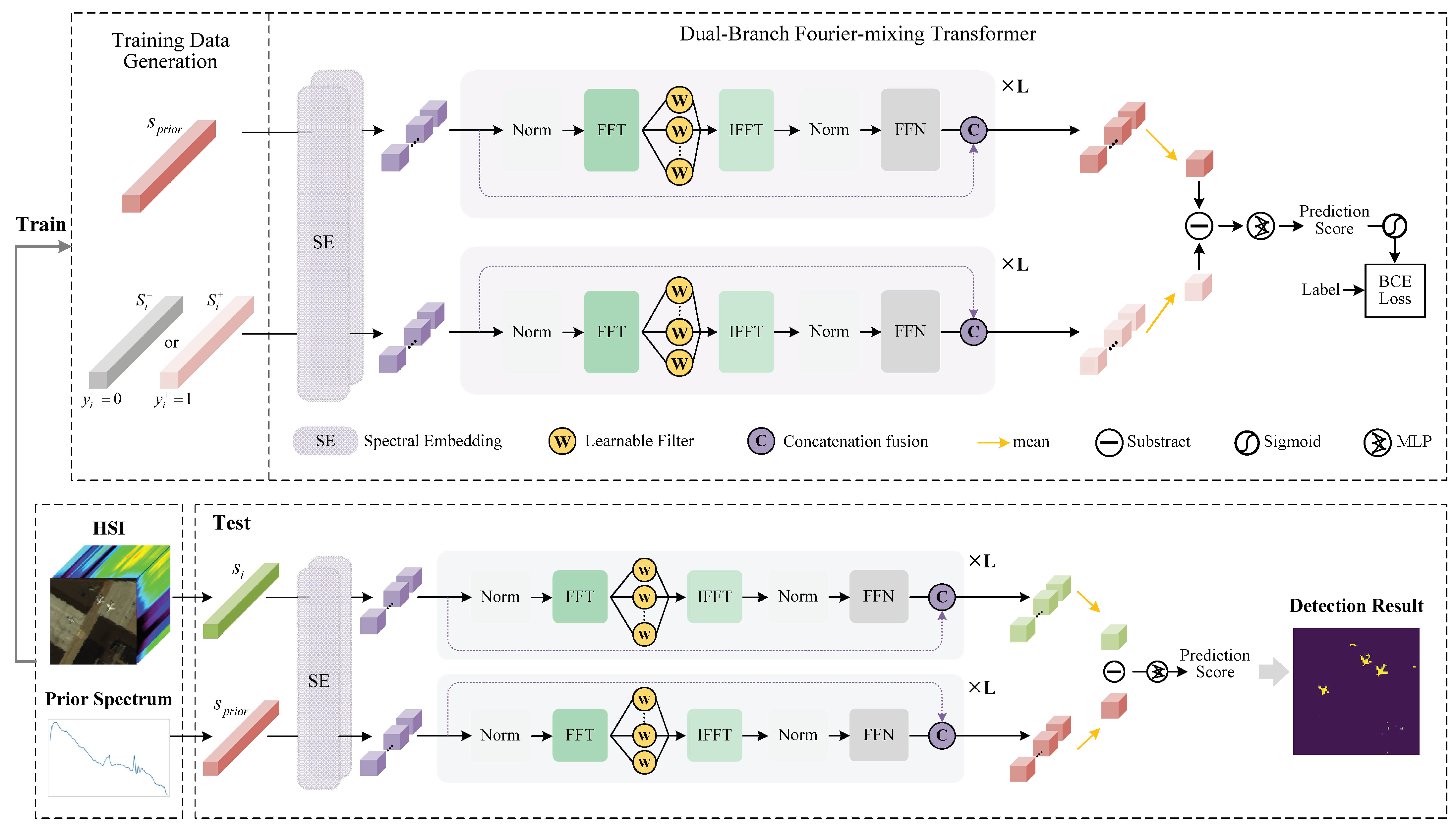
Figure 1 shows an overview of our proposed dual-branch Fourier-mixing transformer-based target detector (DBFTTD). In our work, the target detection task is transformed into the similarity metric learning task, which is realized by the dual-branch architecture consisting of two identical networks that share the same parameters. The training process consists of three main stages: data augmentation, spectral embedding and encoding, and score prediction. First, sufficient and balanced training samples are generated only using the prior target spectrum and the hyperspectral image. Furthermore, the training samples and the prior target spectrum are paired and fed into the dual-branch Fourier-mixing transformer network. The basic building blocks of the Fourier-mixing transformer network consist of spectral embedding, Fourier-mixing with filter ensembles, skip connection, and score prediction. The detailed implementation of the proposed DBFTTD is described as follows.

Figure 1.
Flowchart of the proposed dual-branch Fourier-mixing transformer-based target detector (DBFTTD). In the training stage, data generation provides spectral pairs, and . Then, two spectral sequences in each spectral pair pass through the dual-branch Fourier-mixing transformer network at the same time. , and represent the prior spectrum, target training sample with label , and background training sample with label , respectively. In the testing stage, represents the test spectral sequence in the given HSI, which is paired with the prior target spectrum and the fed into the well-trained network to get the final detection result.
2.2. Construction of Training Samples
For a given HSI with p pixels and n bands, denotes the spectral sequence. The given single target prior spectrum is represented by . Based on the hyperspectral image itself and the single prior spectrum, we construct training samples, including background samples and target samples. The illustration of training data generation in the proposed DBFTTD is shown in Figure 2. Based on the background dominant assumption, all spectral sequences in the given HSI are considered as background samples . Using the given single target prior spectrum, target samples can be obtained by data augmentation.
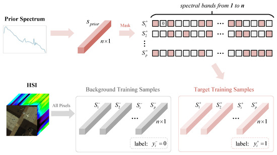
Figure 2.
Illustration of training data generation in the proposed DBFTTD. For a given HSI (with p pixels and n bands) and the single prior spectrum , p target training samples and p background training samples are obtained. The target training samples are obtained by a simple yet efficient dropout strategy, which is applied to along the spectral dimension. Based on the background dominant assumption, all spectral sequences in the given HSI are considered as background training samples .
The target sample augmentation is realized by a simple yet efficient dropout strategy, which is applied to along the spectral dimension for p times. The dropout strategy is inspired by the cutout in [47]. To be specific, a new target sample is obtained by randomly masking some bands in in the spectral dimension. The corresponding values of the masked bands are substituted for zero. After repeating the dropout strategy for p times, the target samples with the same number of background samples are generated to balance positive samples and negative samples.
After obtaining the target samples and background samples, sample pairs need to be constructed for the dual-branch architecture in this work. In the training stage, we generate training pairs as input of the dual-branch Fourier-mixing transformer network using the obtained training samples and the prior target spectrum. Specifically, the input training pairs include the positive training pairs with labels , and the negative training pairs with labels . The positive training pairs and the negative training pairs have the same quantity, leading to balanced data distribution for training. Then the generated training pairs will be fed into the network for training.
2.3. Dual-Branch Fourier-Mixing Transformer
We aim at developing a transformer-style network for HTD that can strike a balance between representation ability and computational efficiency. To achieve this, a Fourier-mixing transformer network with learnable filter ensembles for HTD is proposed. This architecture comprises four parts: spectral embedding, Fourier-mixing with filter ensembles, skip connection, and score prediction. First, the spectral embedding module is designed with a focus on the spectrometric characteristics, extracting local spectral characteristics from multiple adjacent bands. Second, the Fourier-mixing sublayer is designed to capture the contextual relationships between tokens more efficiently, supported by the filter ensembles to improve performance. Third, the skip connection is utilized by concatenating and fusing, reducing information loss in propagation from shallow to deep layers. Furthermore, the score predictor is designed to obtain final prediction scores for training and testing.
2.3.1. Spectral Embedding
A spectral embedding module is utilized with a focus on the spectrometric characteristics, extracting local spectral characteristics from multiple adjacent channels, which is inspired by [43]. Specifically, we take groups of several adjacent channels as input tokens, followed by a trainable linear projection to convert the grouped tokens to embedding vectors. First, groups of several adjacent channels are taken as input tokens. The overlapping grouping operation is utilized to decompose the spectral sequence into
where is the grouped representation of the spectral sequence, which is composed of n tokens of length m. The token is , where indicates the rounding down operation. The scalar n and m are the number of spectral sequence channels and considered adjacent channels. Then a learnable linear transformation converts the grouped representation to the feature embedding of size . Meanwhile, position embedding with the same size as the feature embedding is added. Finally, the resulting embedding vector, , serves as input to the spectral encoder. Note that the scalars n and d serve as the token dimension and the hidden dimension of the input sequence for the spectral encoder, respectively.
2.3.2. Fourier-Mixing with Filter Ensembles
One primary obstacle in applying a typical transformer to HTD lies in the substantial computational cost and memory burden imposed by the multi-head self-attention (MSA) sublayer, leading to less efficient target detection. To improve the computational efficiency, we replace the heavy MSA sublayer with a simpler and more efficient one. We utilize the Fourier transform with accelerated linear transformations as an alternate hidden representation mixing mechanism. The attention-free Fourier-mixing mechanism is designed for mixing information globally and extracting sequential features, supported by the filter ensembles to enhance stability. Specifically, the Fourier-mixing sublayer contains three key operations: (1) Fourier Transform; (2) element-wise multiplication with learnable filter ensembles; (3) inverse Fourier Transform.
We start by introducing the Fourier Transform and the inverse Fourier Transform. The Fourier Transform decomposes a sequence into its constituent frequencies. In terms of practical applications, discrete Fourier transform (DFT) and the Fast Fourier transform algorithm (FFT) play important roles in the field of digital signal processing. The DFT formulation starts with
in which represents the input sequence with . For each k, DFT generates a new representation as a sum of all of the original input tokens . Note that the FFT refers to a class of algorithms for efficiently computing the DFT, the computation complexity can be reduced from to . The inverse Fourier Transformer can recover the original signal from its corresponding frequency-domain representation. The inverse DFT can be formulated as
The inverse DFT can also be efficiently computed using the inverse fast Fourier transform (IFFT).
In the Fourier-mixing sublayer, the first step is the Fourier transform, which is performed by the two-dimensional (2D) FFT. Given the input sequence , with n tokens of hidden dimension d, the 2D FFT can be achieved by repeating the one-dimensional (1D) FFT along the corresponding dimensions. The input sequence z can be converted to the frequency-domain feature Z, which can be formulated as
and are 1D FFTs that are applied along the token dimension and the hidden dimension, respectively. In order to learn the interactions in the frequency domain, we apply element-wise multiplication between the frequency-domain feature Z and the filter ensembles.
where ⊙ is the element-wise multiplication, and is the ith learnable filter, which is inspired by the digital filters in signal processing [48]. The learnable filter is utilized to learn interactions among tokens in the frequency domain, which can represent an arbitrary digital filter in the frequency domain. As the learnable filter is able to interchange information in the frequency domain and globally cover all frequencies, it can capture both long-term and short-term interactions. Inspired by ensemble learning, we designed the learnable filter ensembles with the aim of enhancing their nonlinearity and generalization ability by aggregating multiple learners [46]. We propose a simple but effective ensemble method by integrating the results of E learnable filters . We simply AVG the results and get , the final result of the element-wise multiplication with learnable filter ensembles. Finally, we adopt the IFFT to transform the spectrum back to the spatial domain.
2.3.3. Skip-Layer Connection
The proposed dual-branch network consists of two designed Fourier-mixing transformer encoders with shared structures and parameters. The Fourier-mixing transformer encoder is designed for spectral encoding and is referred to as a spectral encoder below. The spectral encoder is composed of several identical layers, and each layer has two sublayers. The first sublayer is a Fourier-mixing mechanism, and the second sublayer is a fully connected feed-forward network (FFN). The Fourier-mixing sublayer provides the feed-forward sublayer sufficient access to all tokens. The FFN sublayer consists of two linear transformations, with a Gaussian error linear unit (GELU) activation between them. The layernorm is employed before each sublayer. A skip-layer connection is employed after every layer.
The skip connection plays a crucial role in transformers. However, the simple additive skip connection operation only occurs within each transformer block, weakening the connectivity across different layers [43]. To enhance propagation from shallow to deep layers, we make use of skip connections between connected layers by concatenation and fusion. Thereby fostering effective propagation of information without introducing significant loss. The spectral encoder has L layers with identical structures. In the lth layer, represents a nonlinear mapping that maps the input sequence to the output sequence . The shortcut connection is described as follows. The obtained by the mapping operation and the identity mapping of the input sequence are combined by concatenation and fusion
The concatenation operation between sequence vectors is represented by , and can be simply seen as one convolutional layer for fusion. Finally, the output vectors of the last spectral encoder layer are averaged along the hidden dimension to obtain the final output vector, which serves as the spectral feature representation. Furthermore, to avoid ambiguity in symbol representations, it should be noted that by the time , is the initial inputs to the entire spectral encoder.
2.3.4. Score Predictor and Target Detection
Based on the aforementioned construction of the training data, we can obtain sample pairs as input for the dual-branch architecture in this work. In each sample pair, two spectral sequences pass through the dual-branch network, finally giving two extracted spectral feature representations. After that, the two feature representations are subtracted and then fed into MLP to obtain the final prediction score.
For , the positive sample pair and the negative sample pair are fed into the dual-branch network, which is represented by . Based on MLP, we can obtain prediction scores including the positive one and the negative one , where
Once we forgot the prediction scores of sample pairs, we utilize binary cross entropy (BCE) to measure the distance between scores and their corresponding labels. Given the prediction score with label and with label , the BCE loss is formulated as follows to supervise the training process:
where b is the batch size and refers to the sigmoid function. Note that for a batch of size b, there are b positive sample pairs and b negative sample pairs, which leads to balanced training.
In the testing stage, each test spectral sequence in the given HSI is paired with the prior target spectrum. For , each testing pair is fed into the well-trained dual-branch Fourier-mixing transformer network to get the final detection score .
3. Experimental Settings
3.1. Experimental Data Sets
Five images from three public hyperspectral data sets are used for experiments and analysis to evaluate the performance of our proposed algorithm. Given a specific hyperspectral image, hyperspectral target detection tries to detect and locate the specific target under a given prior target spectrum [6]. All five images provide groundtruth maps, but only the Muufl Gulfport data set provides the prior target spectrum. For the Muufl Gulfport data set, the pure endmember target spectrum with laboratory spectrometer measurements is provided in [49]. For data sets without a measured prior spectrum, following the method in [50], we conduct morphological erosion operations on the ground truth maps, and their average spectra represent the prior target spectrum.
3.1.1. San Diego Data Set
The first data set was captured by AVIRIS over the San Diego airport area, CA, USA. It has pixels with 224 spectral bands. Two subimages named San Diego-1 and San Diego-2 are selected from the original HSI data for experiments. In order to maintain consistency and transparency in comparison experiments, we followed the usage of bands as in many previous research studies. Precisely, bands no. 1–6, 33–35, 97, 107–113, 153–166, and 221–224 are considered noisy bands [51]. After removing noisy bands, each of the two subimages has pixels with 189 bands. San Diego-1 contains 134 pixels of three aircrafts as targets, and San Diego-2 contains 57 pixels of three aircrafts as targets. The pseudo-images and the ground-truth maps for San Diego-1 and San Diego-2 are shown in Figure 3 and Figure 4.

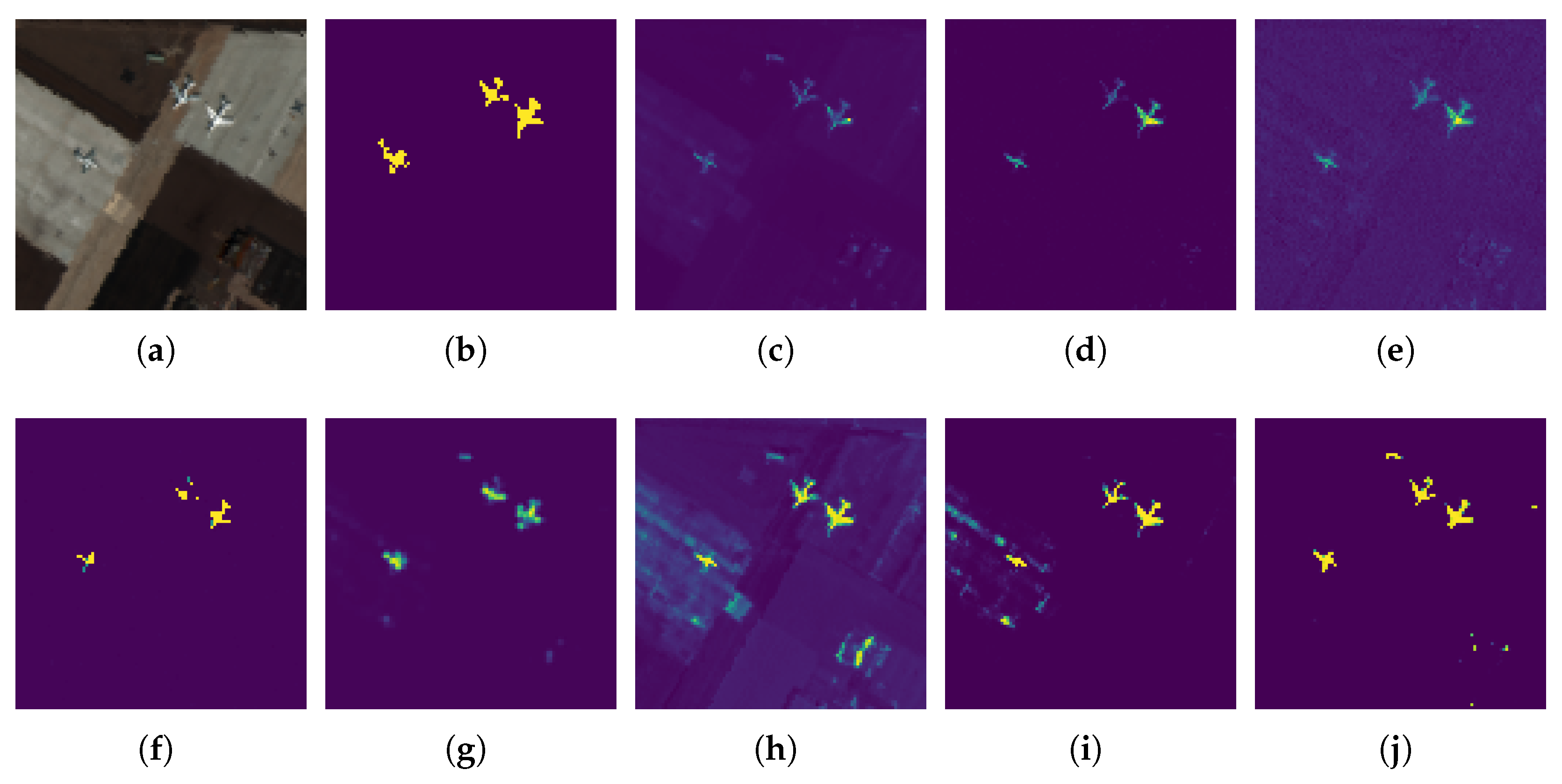
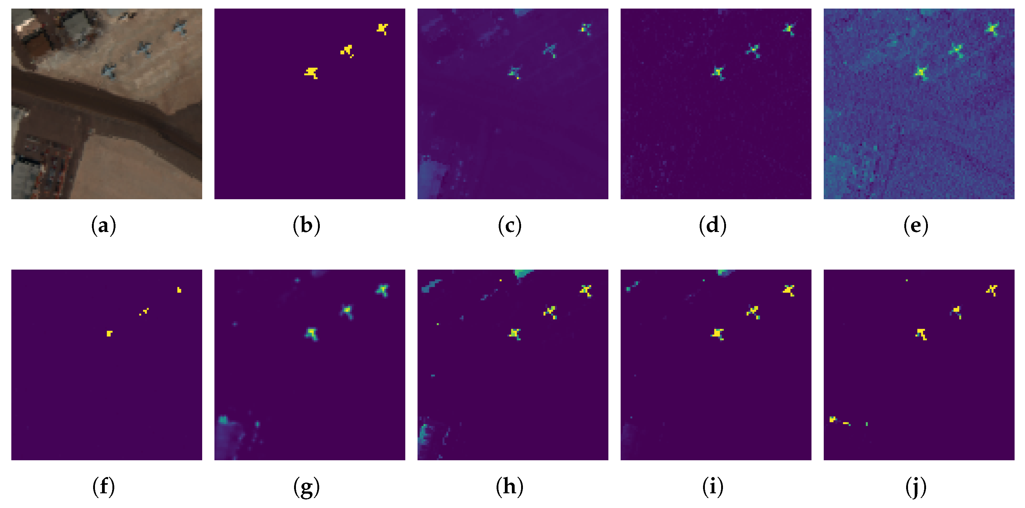
Figure 3.
San Diego-1 scene and detection maps of different comparison methods. (a) False color image, (b) Ground truth, (c) SAM, (d) ACE, (e) CEM, (f) E-CEM, (g) HTD-IRN, (h) SFCTD, (i) TSCNTD, (j) Ours.

Figure 4.
San Diego-2 scene and detection maps of different comparison methods. (a) False color image, (b) Ground truth, (c) SAM, (d) ACE, (e) CEM, (f) E-CEM, (g) HTD-IRN, (h) SFCTD, (i) TSCNTD, (j) Ours.
3.1.2. Airport-Beach-Urban (ABU) Data Set
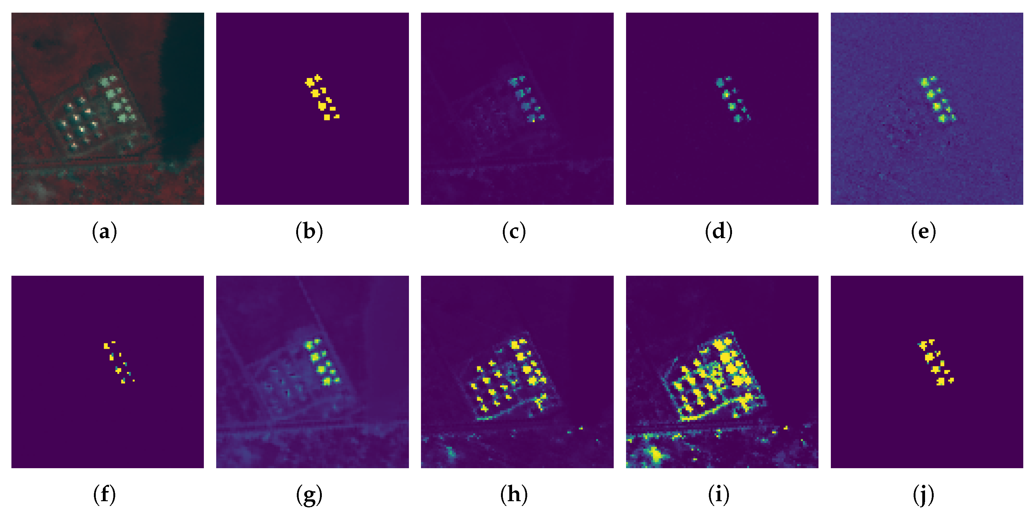
The second data set is the ABU data set, which is publicly available in [7]. Two images from the urban scene in the ABU data set are used to test our proposed method. According to the downloaded data, it is available to describe the two urban scene images named Urban-1 and Urban-2. Each of the two urban images was captured by an Airborne Visible/Infrared Imaging Spectrometer (AVIRIS) with a spatial size of pixels. Urban-1 has 204 bands, containing 67 pixels of nine buildings as targets. Urban-2 has 207 bands, and 88 pixels of nine buildings were regarded as targets. The pseudo-images and the ground-truth maps for Urban-1 and Urban-2 are shown in Figure 5 and Figure 6.
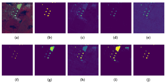
Figure 5.
Urban-1 scene and detection maps of different comparison methods. (a) False color image, (b) Ground truth, (c) SAM, (d) ACE, (e) CEM, (f) E-CEM, (g) HTD-IRN, (h) SFCTD, (i) TSCNTD, (j) Ours.
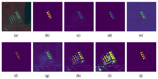
Figure 6.
Urban-2 scene and detection maps of different comparison methods. (a) False color image, (b) Ground truth, (c) SAM, (d) ACE, (e) CEM, (f) E-CEM, (g) HTD-IRN, (h) SFCTD, (i) TSCNTD, (j) Ours.
3.1.3. MUUFL Gulfport Data Set
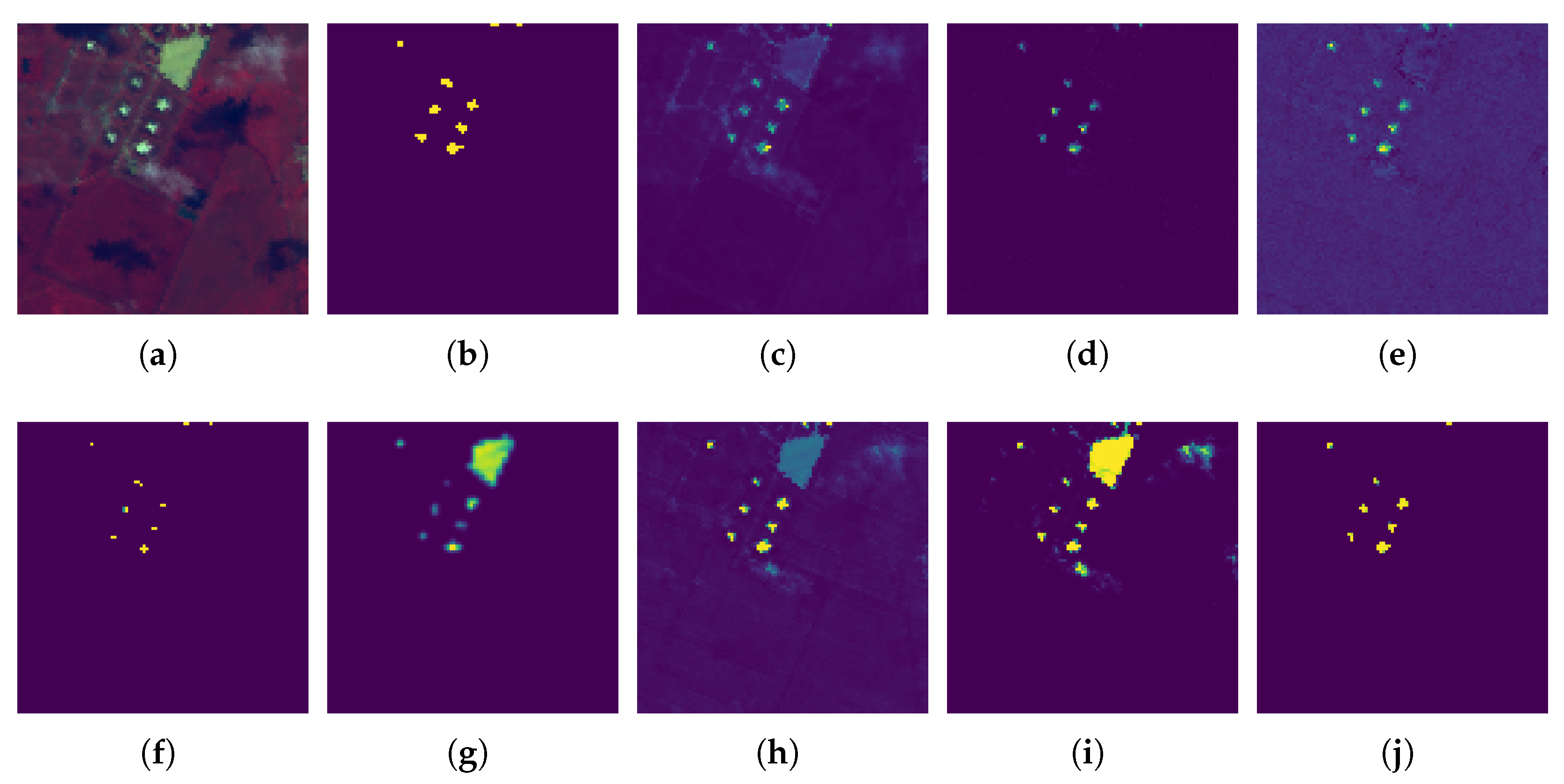
The third data set is the MUUFL Gulfport data set [49], which was acquired using a Compact Airborne Spectrographic Imager (CASI-1500) over the Gulf Park Campus of the University of Southern Mississippi. The original MUUFL Gulfport data set has 325 × 337 pixels with 72 spectral bands, and the scene and scene labels are publicly available in [49,52]. The lower right corner of the original image contains an invalid area; thus, only the first 220 columns were used, and the first four and last four bands were removed due to noise. Thus, the size of the cropped MUUFL Gulfport is 325 × 220 × 64, containing 269 pixels of several cloth panels as targets to be detected, and the pure endmember target spectrum with laboratory spectrometer measurements is provided in [49]. The pseudo-image and the ground-truth map for Muufl Gulfport are shown in Figure 7.
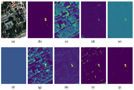
Figure 7.
Muufl Gulfport scene and detection maps of different comparison methods. (a) False color image, (b) Ground truth, (c) SAM, (d) ACE, (e) CEM, (f) E-CEM, (g) HTD-IRN, (h) SFCTD, (i) TSCNTD, (j) Ours.
3.2. Assessment Criteria
Three criteria are utilized to evaluate the performance of our proposed target detection method, including the receiver operating characteristic (ROC) curve, the area under the ROC curve (AUC) value, and the probability of detection under the false alarm rate (PD under FAR). The ROC curve is a plot based on probability of detection (PD) versus false alarm rate (FAR) under different threshold settings on the detection probability map [53]. FAR and PD are formulated as
where is the number of correctly detected target pixels, is the number of real target pixels, is the number of falsely detected target pixels, and is the number of background pixels.
The area under the ROC curve of PD and FAR, , is utilized to quantitatively evaluate the detection performance of a detector [54].
According to [55,56], apart from , another two AUC indicators including and are calculated as follows:
In addition, , , and can further be used to design some other quantitative detection indicators, including for background suppressibility, for target detectability, for overall detection accuracy and signal-to-noise probability ratio (SNPR) [55]. Where
Furthermore, PD under FAR is the specific PD under a fixed, low FAR [57]. A robust detector should not only highlight targets but also suppress backgrounds, so the PD under FAR is a valid indicator to show the effectiveness of the detector. In this work, the PD under FAR = 0.01 of different comparison methods on four data sets is provided. Generally speaking, the higher the value of PD under a low FAR, the better the detection performance of the detector.
3.3. Comparison Methods and Parameter Setup
To validate the effectiveness of the proposed DBFTTD, four widely used classical methods (SAM, ACE, CEM, and E-CEM [46]) and three advanced deep learning-based methods (Transformer-based HTD-IRN [40], CNN-based TSCNTD [37], and FCNN-based SFCTD [50]) are adopted for comparison. HTD-IRN is an interpretable representation network-based target detector with Tranformer and learnable background subspace; TSCNTD is a two-stream convolutional network-based target detector; and SFCTD is a siamese fully connected-based target detector. The settings of deep learning-based methods for comparison are consistent with the original work.
For the proposed DBFTTD, we utilize the Adam optimizer for all the experiments; the batch size is 128, the learning rate is 0.0001, and the dropout rate is 0.1. All the experiments are run on pytorch 1.9.0 with a CPU of Intel (R) Core (TM) i9-10900X @ 3.70 GHz, 32 GB of RAM, and a GPU of NVIDIA GeForce RTX 3090.
4. Experimental Results and Analysis
4.1. Detection Performance Comparison
In this section, to validate the effectiveness of the proposed DBFTTD, we present and analyze the detection performance comparisons for different detectors, including detection maps, ROC curves, AUC values, and PD under FAR.
4.1.1. Detection Maps Comparison
Figure 3, Figure 4, Figure 5, Figure 6 and Figure 7 show the detection maps of different comparison methods on five data sets. It can be found that, compared with other detectors, DBFTTD achieves balance in highlighting targets and suppressing backgrounds. In DBFTTD, the target detection task is transformed into the similarity metric learning task. The main reason for the good performance of DBFTTD is that the learnable filters are able to learn the interactions among tokens in the Fourier domain and globally cover all frequencies, thus capturing both long-term and short-term spectral features that simple measures in the feature space directly correspond to spectra similarities.
For San Diego-1, the maps of detection results for different detectors are shown in Figure 3. For detection of the two upper right aircrafts, SFCTD, TSCNTD, and the proposed DBFTTD can highlight target pixels and maintain the morphological integrity of targets, while the first five detectors achieve ambiguous detection results. Although E-CEM can highlight some target pixels and suppress almost all background pixels, it fails to describe the shape of the target. For the lower left aircraft, the proposed DBFTTD achieves high detection scores and retains the integrity of targets, while SFCTD and TSCNTD fail to. It’s worth noting that ACE suppresses the detection scores of background pixels to extremely low levels, but only a few target pixels are highlighted. Among all the detectors, the proposed DBFTTD is better at highlighting targets, including target margins, and demonstrates high separability between backgrounds and targets.
For San Diego-2, the maps of detection results for different detectors are shown in Figure 4. SAM, ACE, CEM, and HTD-IRN achieve ambiguous detection results and show low visualization contrast. E-CEM can only highlight several pixels in the middle of targets. SFCTD, TSCNTD, and DBFTTD can locate and highlight targets and achieve similar detection results, and TSCNTD and DBFTTD are slightly better at highlighting target margins than SFCTD.
For Urban-1, the maps of detection results for different detectors are shown in Figure 5. TSCNTD and DBFTTD show higher visualization contrast than the first six detectors. However, TSCNTD mistakenly highlights a great deal of background pixels, reflecting poor background suppression. It should be particularly noted that the proposed DBFTTD achieves an outstanding balance between target detection and background suppression.
For Urban-2, the maps of detection results for different detectors are shown in Figure 6. E-CEM, SFCTD, TSCNTD, and ours show better visualization contrast than the first five detectors. Although E-CEM performs well in suppressing backgrounds, it fails to highlight the edge of targets. Although SFCTD and TSCNTD perform well in highlighting targets, they perform poorly in suppressing backgrounds and have high false alarm rates. Among all the detectors, our DBFTTD not only detects target pixels with excellent scores but also suppresses backgrounds to an extremely low level.
For Muufl-Gulfport, the maps of detection results for different detectors are shown in Figure 7. The last four detectors show better visualization contrast than the other four detectors. However, HTD-IRN achieves poor background suppression and ignores the taget at bottom right. SFCTD ignores the target on the top right, and TSTNTD ignores the target on the bottom left. Among all the detectors, our DBFTTD not only detects target pixels with excellent scores but also suppresses backgrounds to an extremely low level.
4.1.2. ROC Curves Comparison
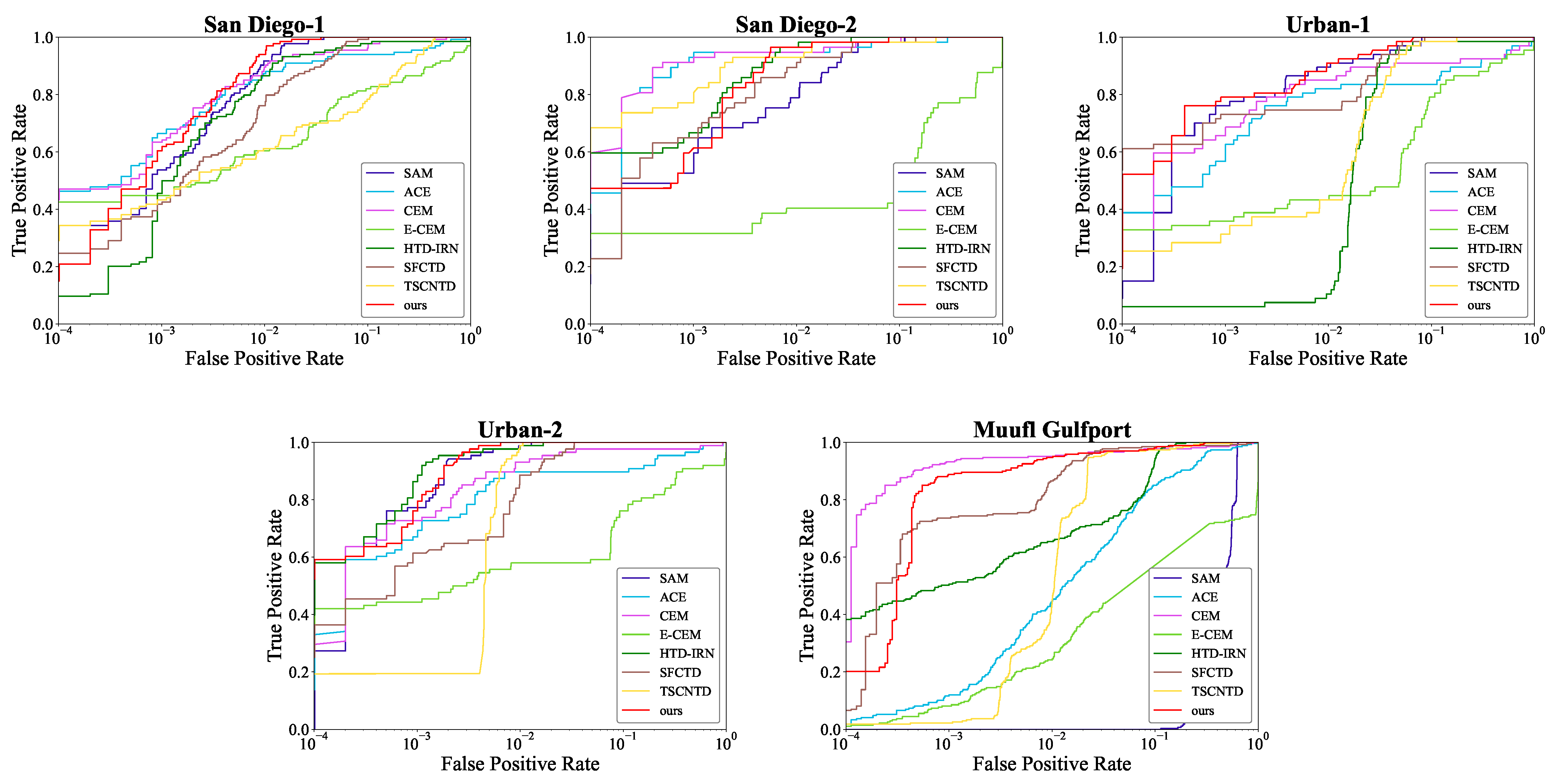
The ROC curves of comparison methods on five data sets are shown in Figure 8. The red curves represent the ROC curves of the proposed DBFTTD. Firstly, there is the analysis of the underperforming curves. The ACE, CEM, and MF always achieve low detection probability when the false alarm rate reaches 1 for San Diego-1 and the two urban data sets; TSCNTD gets low detection probability in most false alarm rate; SFCTD is inferior to the proposed DBFTTD within the surrounding range of the false alarm rate . Secondly, there is the analysis of the curves of the proposed DBFTTD. For the two San Diego data sets, although the proposed DBFTTD gets a lower detection probability at the beginning, it gets the most rapid rise as the curve grows. For the Urban-1 data set, our curve is lower than the curve of SFCTD, around false alarm rate, but it achieves competitive detection probability as the growth of the false alarm rate increases. For the Urban-2 data set, our curve achieves the lowest false rate when the detection probability reaches 1 (detects all targets). For the Muufl Gulfport data set, our curve is located in the upper left corner compared to the other three deep learning-based detectors, which indicates its promising performance.
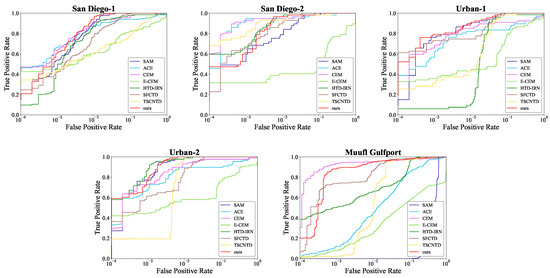
Figure 8.
ROC curves of different comparison methods on the five data sets.
4.1.3. AUC Values Comparison
In addition, in order to quantitatively evaluate the performance of different methods, the values of various AUC indicators on the five data sets are shown in Table 1, Table 2, Table 3, Table 4 and Table 5. In these tables, the optimal values are bolded, and the suboptimal values are underlined.

Table 1.
AUC Values’ Comparison for San Diego-1.
Table 2.
AUC Values’ Comparison for San Diego-2.
Table 3.
AUC Values’ Comparison for Urban-1.
Table 4.
AUC Values’ Comparison for Urban-2.
Table 5.
AUC Values’ Comparison for Muufl Gulfport.
For the two San Diego data sets, the AUC values are shown in Table 1 and Table 2. The proposed DBFTTD obtains the optimal values except for San Diego-1. Although ACE obtains the optimal for San Diego-1 because it suppresses background pixels to very low levels, it performs poorly on other AUC values since it fails to highlight target pixels. For the two urban data sets, the AUC values are shown in Table 3 and Table 4. The proposed DBFTTD markedly outperforms other comparison methods in terms of and that reflect background suppressibility, as well as and SNPR for overall performance. SFCTD and TSCNTD achieve superior and as they present strong target detectability; however, they falsely highlight an awful lot of background pixels while highlighting target pixels. Among all the detectors for comparison, the proposed DBFTTD achieves competitive performance in various AUC values, presenting an outstanding balance between target detection and background suppression. For the Muufl Gulfport data set, the AUC values are shown in Table 5. It is evident that the proposed DBFTTD produces the most accurate and robust results of the seven metrics compared to other detectors.
4.1.4. PD under FAR Comparison
Moreover, the PD under FAR = 0.01 of different comparison methods on five data sets are provided to assess the effectiveness and robustness of the DBFTTD, as illustrated in Table 6. As shown, the proposed DBFTTD achieves the highest PD values under FAR = 0.01 in the first four data sets. Note in particular that the PD value of DBFTTD is up to 1 in the Urban-2 data set, significantly better than 0.9886 of the suboptimal ones.
Table 6.
PD under FAR = 0.01 of different comparison methods on five data sets.
4.2. Comparison with the Original Transformer
4.2.1. Analysis of the Skip-Layer Connection
In Transformer, the simple additive skip connection operation only occurs within each Transformer block. To enhance propagation from shallow to deep layers, we make use of skip connections between connected layers by concatenation and fusion. To verify the effectiveness of the skip-layer connection, ablation experiments were performed on five datasets. The experimental settings are consistent with the DBFTTD, except for the component of the ablation study. Figure 9 and Figure 10 display the detection maps and the corresponding ROC curves on the five datasets, respectively.
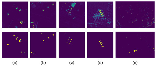
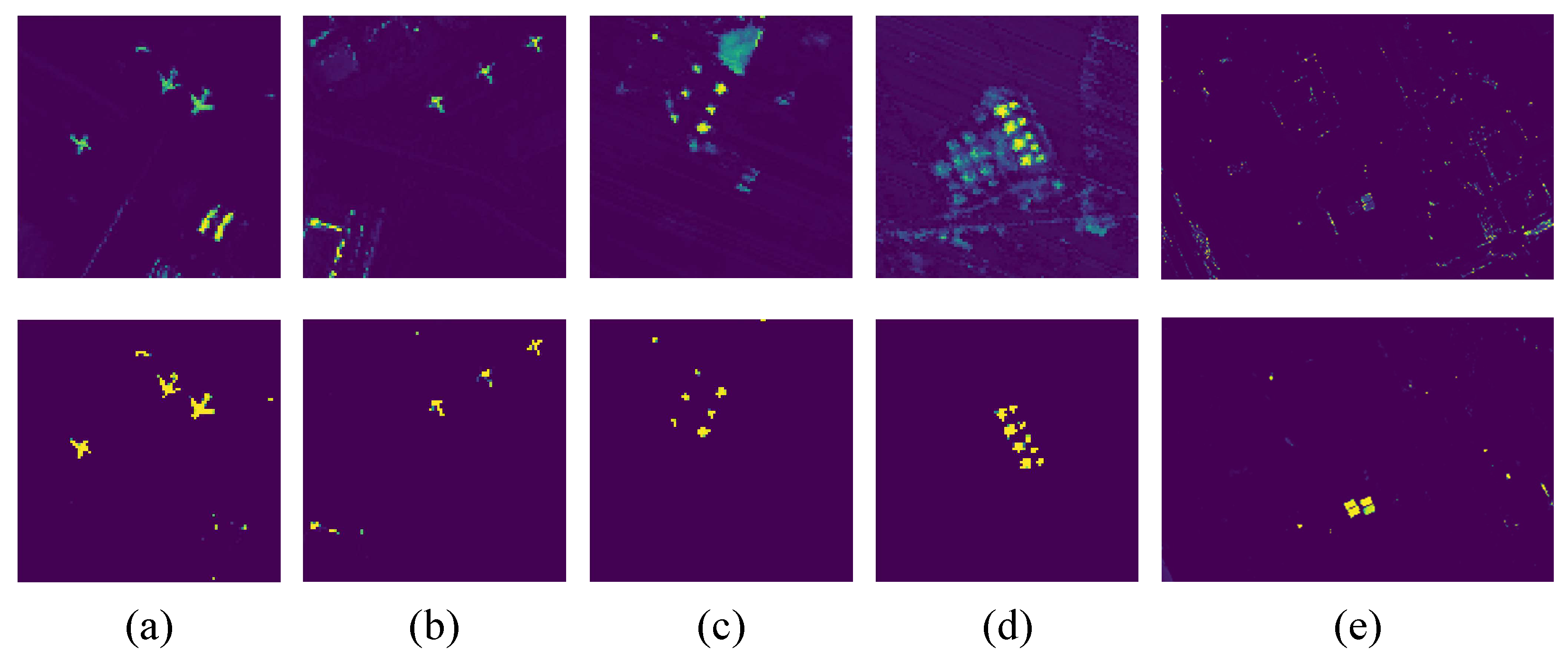
Figure 9.
Comparison of detection maps without skip-layer connection and with skip-layer connection for five data sets. (a) San Diego-1. (b) San Diego-2. (c) Urban-1. (d) Urban-2. (e) Muufl Gulfport. First row: without skip-layer connection. Second row: with skip-layer connection.
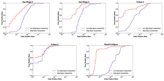
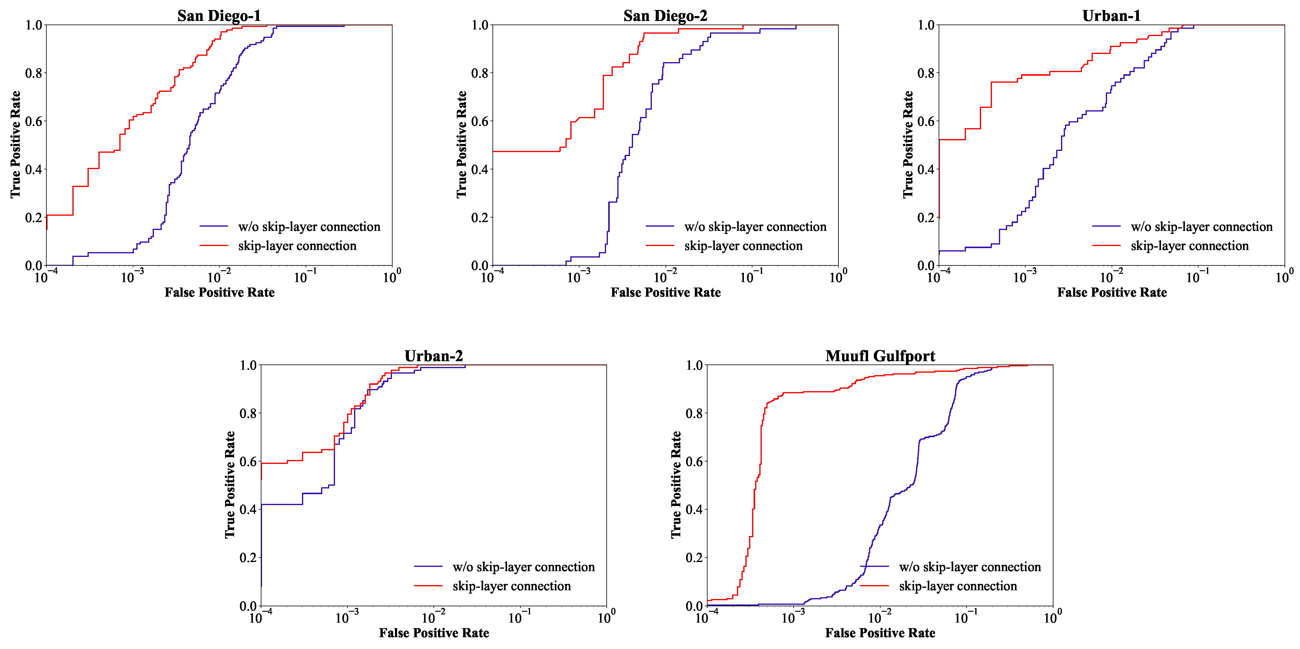
Figure 10.
Comparison of ROC curves without skip-layer connection and with skip-layer connection for five data sets.
According to the detection maps on Muufl Gulfport, the variant without skip-layer connection has extremely poor performance because it fails to locate and highlight target pixels. In the case of other images, the variant can locate and maintain the shape of targets, but it fails to highlight them obviously. Moreover, the variant is inferior in suppressing backgrounds, and many background pixels are incorrectly detected with high detection scores. As shown in Figure 10, for all five data sets, the ROC curves of the DBFTTD are much closer to the upper left than the variant. By comparison, the proposed DBFTTD outperforms the variant without the skip-layer connection, demonstrating the necessity and effectiveness of the skip-layer connection.
4.2.2. Analysis of the Fourier-Mixing Module and the Self-Attention Module
The considerable computation complexity of self-attention has been a persistent challenge when applying Transformer models to vision tasks [58]. Since the Fourier Transform has previously been used to speed up transformers [44,45], we replace the attention module in transformers with the Fourier-mixing module for efficient HTD. To verify the effectiveness of the Fourier-mixing module, ablation experiments are performed on five datasets. Figure 11 and Figure 12 display the detection maps and the corresponding ROC curves on the five datasets, respectively.
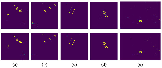
Figure 11.
Comparison of detection maps with attention module and Fourier-mixing module for five data sets. (a) San Diego-1. (b) San Diego-2. (c) Urban-1. (d) Urban-2. (e) Muufl Gulfport. First row: attention-based. Second row: Fourier-based.
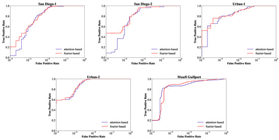
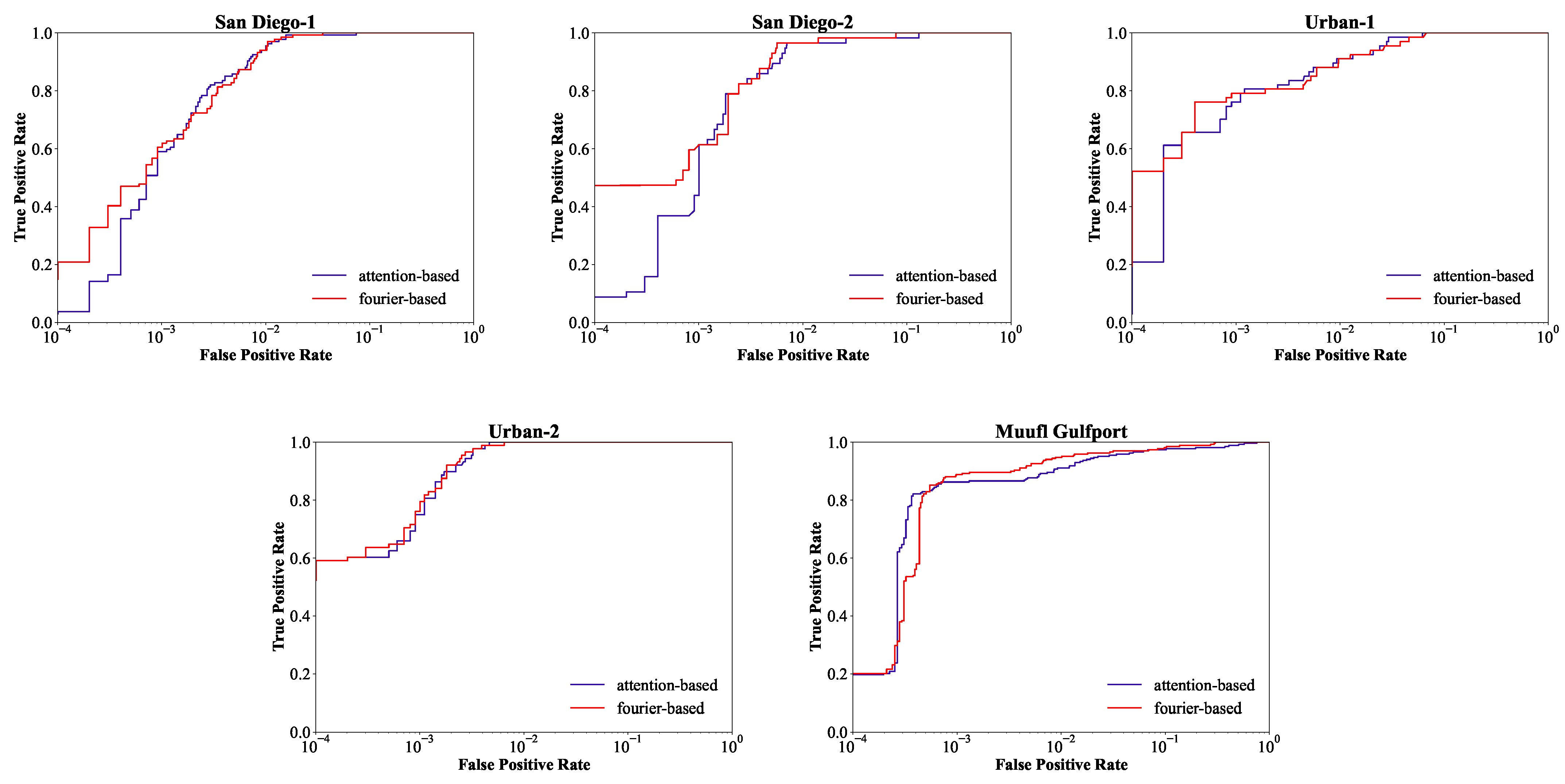
Figure 12.
Comparison of ROC curves with attention module and Fourier-mixing module for five data sets.
In Figure 11, the first row is based on the self-attention module, and the second row is based on the Fourier-mixing module. The detection maps in the two rows generally have similar visual contrast. Both the attention-based detector and the Fourier-based detector can highlight targets and describe the shape approximately, as well as suppress backgrounds to low levels. However, by replacing the self-attention module with the Fourier-mixing module, the second row is slightly better than the first row for San Diego-1 and Muufl Gulfport. For San Diego-1, based on the attention module, several pixels at the edge of airplanes get lower confidence than pixels in the middle of airplanes. For Muufl Gulfport, based on the Fourier-mixing module, the upper left target becomes clearer and more prominent. As shown in Figure 12, the ROC curves can qualitatively evaluate the performance. For the first three data sets, the ROC curve based on the Fourier-mixing module is the closest to the top left corner. For Urban-2, the two ROC curves are almost overlapping, so both methods can achieve good performance. For Muufl Gulfport, the detection rate based on the Fourier-mixing module is competitive under the low FPR from to 0. By comparison, the Fourier-based detector performs as well as the attention-based detector and even slightly better; thus, the Fourier-mixing module is demonstrated effective.
4.2.3. Time Analysis
In our work, the Fourier-mixing sublayer replaces the heavy MSA sublayer in transformers to speed up the transformer-style network for HTD. In this section, we analyze the time cost of our attention-free DBFTTD and the attention-based variant to illustrate the efficiency of our proposed method. For fair comparison, the settings are consistent except for the component of the ablation study, and we analyze their inference time in the test stage on the four researched data sets. The time costs of the attention-free DBFTTD and the attention-based variant are listed in Table 7.
Table 7.
Inference time (in milliseconds) comparison of our attention-free DBFTTD and the attention-based variant on the four data sets.
San Diego and ABU data sets have a spatial size of , and the difference in time cost between the different data sets is mainly caused by the number of bands. The San Diego-1 and San Diego-2 have 189 bands, while Urban-1 has 204 bands and Urban-2 has 207 bands. From the perspective of the data size, the image with more bands costs more time since the designed network needs to extract more features. The proposed DBFTTD saves more time than the attention-based variant in all four data sets. The average inference time of DBFTTD is about 120 ms shorter than that of the attention-based variant. DBFTTD runs faster than it is capable of speeding up the transformer-style architecture, which demonstrates the improvement in efficiency.
4.3. Parameter Sensitivity Analysis
4.3.1. Analysis of Filter Ensembles
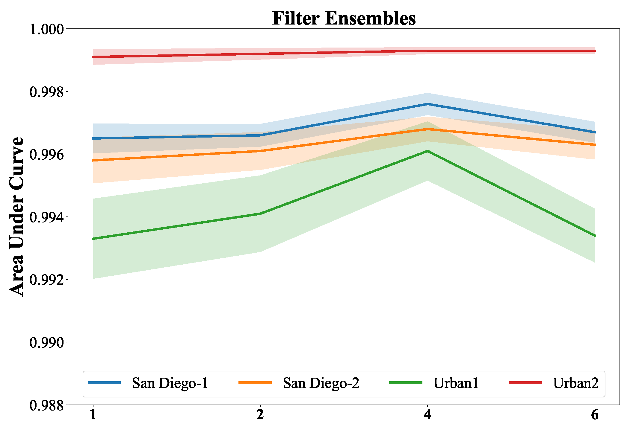
Figure 13 shows the parameter sensitivity analysis of the number of filter ensembles. For the setting of each number, we repeat ten times and compute the means and standard deviations of the AUC values. The dark and light color plots represent the AUC value means and standard deviation, respectively. The results of four data sets are painted with different colors. As the number increases, the variance represented by the light regions gradually decreases, indicating improved stability. Moreover, it is obvious that the AUC values of number 4 are better than the others. Therefore, Filter ensembles enhance the generalization ability and improve the detection performance, and the default ensemble number in our proposed DBFTTD is 4.

Figure 13.
The parameters sensitivity analysis of the number of the filter ensembles for four data sets. The default ensemble number in our proposed DBFTTD is 4.
4.3.2. Analysis of Dropout for Data Augmentation
The AUC values of the DBFTTD with different dropout rates for data augmentation for four data sets are shown in Figure 14. For San Diego-1, San Diego-2, and Urban-1, the AUC values of different dropout rates from 0 to 0.5 reveal that the detection performance is better when the dropout rate is set at 0.1. For Urban-2, the AUC values can prove that the dropout rate for data augmentation is not sensitive, and the detection performances are promising under both the six dropout rates. This is because the backgrounds in Urban-2 can be easily distinguished from targets even by the simplest matching method, SAM, as shown in the detection map shown in Figure 6. Furthermore, the original prior target spectrum is sufficient to extract the main information for distinguishing targets and backgrounds. Therefore, the default dropout rate for data augmentation is 0.1.
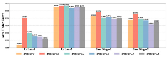
Figure 14.
AUC values of the DBFTTD with different dropout rate for data augmentation for four data sets. The default dropout rate in our proposed DBFTTD is 0.1.
5. Conclusions
In this article, we propose a dual-branch Fourier-mixing transformer network with learnable filter ensembles for hyperspectral target detection, supported by a simple yet effective data augmentation method. First, the proposed transformer-style detector utilizes a Fourier-mixing sublayer to replace the MSA sublayer in the transformer, and adaptive improvements to the transformer such as spectral embedding and skip-layer connection are utilized. Second, this work proposes learnable filter ensembles in the Fourier domain inspired by ensemble learning in E-CEM, which improve detection performance. Moreover, supported by a dropout strategy for data augmentation, the proposed dual-branch network is effectively optimized by the sufficient and balanced target and background spectral pairs generated. Experiments and comparisons with five widely used classical methods and two advanced deep learning-based methods, conducted quantitatively and qualitatively, show that the proposed DBFTTD achieves excellent detection performance. The time-cost comparisons of the attention-free DBFTTD and the attention-based variant show that the DBFTTD is capable of speeding up the transformer-style architecture, which demonstrates the improvement in efficiency. Therefore, the proposed transformer-style detector does well in both detection performance and computational efficiency.
Further research will be conducted for the application of detecting the same targets appearing in different HSIs under different environmental conditions, as well as balancing both effectiveness and efficiency.
Author Contributions
Conceptualization, J.J. and Z.G.; methodology, J.J. and Z.G.; software, J.J.; validation, J.J.; formal analysis, J.J. and Z.G.; investigation, J.J. and Z.G.; resources, P.Z.; writing—original draft preparation, J.J. and Z.G.; writing—review and editing, J.J., Z.G. and P.Z.; visualization, J.J. and Z.G.; supervision, P.Z.; project administration, P.Z.; funding acquisition, P.Z. All authors have read and agreed to the published version of the manuscript.
Funding
This work was partially supported by the National Natural Science Foundation of China (Grant Nos. 61971428 and 62001502).
Institutional Review Board Statement
Not applicable.
Informed Consent Statement
Not applicable.
Data Availability Statement
Hyperspectral data is available at http://xudongkang.weebly.com/data-sets, accessed on 12 August 2023.
Conflicts of Interest
The authors declare no conflict of interest.
References
- Landgrebe, D. Hyperspectral image data analysis. IEEE Signal Process. Mag. 2002, 19, 17–28. [Google Scholar] [CrossRef]
- Bioucas-Dias, J.M.; Plaza, A.; Camps-Valls, G.; Scheunders, P.; Nasrabadi, N.; Chanussot, J. Hyperspectral remote sensing data analysis and future challenges. IEEE Geosci. Remote Sens. Mag. 2013, 1, 6–36. [Google Scholar] [CrossRef]
- Wang, Q.; Lin, J.; Yuan, Y. Salient band selection for hyperspectral image classification via manifold ranking. IEEE Trans. Neural Netw. Learn. Syst. 2016, 27, 1279–1289. [Google Scholar] [CrossRef]
- Zhong, P.; Gong, Z.; Shan, J. Multiple Instance Learning for Multiple Diverse Hyperspectral Target Characterizations. IEEE Trans. Neural. Netw. Learn Syst. 2020, 31, 246–258. [Google Scholar] [CrossRef]
- Yuan, Y.; Lin, J.; Wang, Q. Hyperspectral Image Classification via Multitask Joint Sparse Representation and Stepwise MRF Optimization. IEEE Trans. Cybern. 2016, 46, 2966–2977. [Google Scholar] [CrossRef] [PubMed]
- Nasrabadi, N.M. Hyperspectral target detection: An overview of current and future challenges. IEEE Signal Process. Mag. 2013, 31, 34–44. [Google Scholar] [CrossRef]
- Kang, X.; Zhang, X.; Li, S.; Li, K.; Li, J.; Benediktsson, J.A. Hyperspectral anomaly detection with attribute and edge-preserving filters. IEEE Trans. Geosci. Remote Sens. 2017, 55, 5600–5611. [Google Scholar] [CrossRef]
- Liu, S.; Marinelli, D.; Bruzzone, L.; Bovolo, F. A Review of Change Detection in Multitemporal Hyperspectral Images: Current Techniques, Applications, and Challenges. IEEE Geosci. Remote Sens. Mag. 2019, 7, 140–158. [Google Scholar] [CrossRef]
- Shimoni, M.; Haelterman, R.; Perneel, C. Hypersectral Imaging for Military and Security Applications: Combining Myriad Processing and Sensing Techniques. IEEE Geosci. Remote Sens. Mag. 2019, 7, 101–117. [Google Scholar] [CrossRef]
- Axelsson, M.; Friman, O.; Haavardsholm, T.V.; Renhorn, I. Target detection in hyperspectral imagery using forward modeling and in-scene information. ISPRS J. Photogramm. Remote Sens. 2016, 119, 124–134. [Google Scholar] [CrossRef]
- Kumar, S.; Torres, C.; Ulutan, O.; Ayasse, A.; Roberts, D.; Manjunath, B.S. Deep Remote Sensing Methods for Methane Detection in Overhead Hyperspectral Imagery. In Proceedings of the IEEE Winter Conference on Applications of Computer Vision, Snowmass, CO, USA, 1–5 March 2020; pp. 1776–1785. [Google Scholar]
- Lu, B.; Dao, P.D.; Liu, J.; He, Y.; Shang, J. Recent Advances of Hyperspectral Imaging Technology and Applications in Agriculture. Remote Sens. 2020, 12, 2659. [Google Scholar] [CrossRef]
- Schowengerdt, R.A. Remote Sensing: Models and Methods for Image Processing; Elsevier: Amsterdam, The Netherlands, 2006. [Google Scholar]
- Chang, C.I. An information-theoretic approach to spectral variability, similarity, and discrimination for hyperspectral image analysis. IEEE Trans. Inf. Theory 2000, 46, 1927–1932. [Google Scholar] [CrossRef]
- Manolakis, D.; Shaw, G. Detection algorithms for hyperspectral imaging applications. IEEE Signal Process. Mag. 2002, 19, 29–43. [Google Scholar] [CrossRef]
- Manolakis, D.; Truslow, E.; Pieper, M.; Cooley, T.; Brueggeman, M. Detection algorithms in hyperspectral imaging systems: An overview of practical algorithms. IEEE Signal Process. Mag. 2013, 31, 24–33. [Google Scholar] [CrossRef]
- Kelly, E. An Adaptive Detection Algorithm. IEEE Trans. Aerosp. Electron. Syst 1986, AES-22, 115–127. [Google Scholar] [CrossRef]
- Kraut, S.; Scharf, L.L.; Butler, R.W. The adaptive coherence estimator: A uniformly most-powerful-invariant adaptive detection statistic. IEEE Trans. Signal Process. 2005, 53, 427–438. [Google Scholar] [CrossRef]
- Manolakis, D.; Lockwood, R.; Cooley, T.; Jacobson, J. Is there a best hyperspectral detection algorithm? SPIE 2009, 7334, 733402. [Google Scholar]
- Farrand, W.H.; Harsanyi, J.C. Mapping the distribution of mine tailings in the Coeur d’Alene River Valley, Idaho, through the use of a constrained energy minimization technique. Remote Sens. Environ. 1997, 59, 64–76. [Google Scholar] [CrossRef]
- Ren, H.; Chang, C.I. Target-constrained interference-minimized approach to subpixel target detection for hyperspectral images. Opt. Eng. 2000, 39, 3138–3145. [Google Scholar] [CrossRef]
- Gong, Z.; Zhong, P.; Yu, Y.; Hu, W.; Li, S. A CNN with multiscale convolution and diversified metric for hyperspectral image classification. IEEE Trans. Geosci. Remote Sens. 2019, 57, 3599–3618. [Google Scholar] [CrossRef]
- Gong, Z.; Zhong, P.; Hu, W. Statistical loss and analysis for deep learning in hyperspectral image classification. IEEE Trans. Neural Netw. Learn. Syst. 2021, 32, 322–333. [Google Scholar] [CrossRef]
- Sun, L.; Zhao, G.; Zheng, Y.; Wu, Z. Spectral-Spatial Feature Tokenization Transformer for Hyperspectral Image Classification. IEEE Trans. Geosci Remote Sens. 2022, 60, 5522214. [Google Scholar] [CrossRef]
- Su, H.; Wu, Z.; Zhang, H.; Du, Q. Hyperspectral anomaly detection: A survey. IEEE Geosci. Remote Sens. Mag. 2021, 10, 64–90. [Google Scholar] [CrossRef]
- Hu, M.; Wu, C.; Zhang, L.; Du, B. Hyperspectral Anomaly Change Detection Based on Autoencoder. IEEE J. Sel. Top. Appl. Earth Observ. Remote Sens. 2021, 14, 3750–3762. [Google Scholar] [CrossRef]
- Han, Z.; Hong, D.; Gao, L.; Zhang, B.; Chanussot, J. Deep half-siamese networks for hyperspectral unmixing. IEEE Geosci. Remote Sens. Lett. 2021, 18, 1996–2000. [Google Scholar] [CrossRef]
- Qu, Y.; Qi, H. UDAS: An untied denoising autoencoder with sparsity for spectral unmixing. IEEE Trans. Geosci. Remote Sens. 2018, 57, 1698–1712. [Google Scholar] [CrossRef]
- Chen, B.; Liu, L.; Zou, Z.; Shi, Z. Target Detection in Hyperspectral Remote Sensing Image: Current Status and Challenges. Remote Sens. 2023, 15, 3223. [Google Scholar] [CrossRef]
- Gu, J.; Wang, Z.; Kuen, J.; Ma, L.; Shshroudy, A.; Shuai, B.; Liu, I.; Wang, X.; Wang, G.; Cai, J.; et al. Recent advances in convolutional neural networks. Pattern Recognit. 2018, 77, 354–377. [Google Scholar] [CrossRef]
- Sun, X.; Wang, P.; Wang, C.; Liu, Y.; Fu, K. PBNet: Part-based convolutional neural network for complex composite object detection in remote sensing imagery. ISPRS J. Photogramm. Remote Sens. 2021, 173, 50–65. [Google Scholar] [CrossRef]
- Xu, Q.; Li, Y.; Zhang, M.; Li, W. COCO-Net: A Dual-Supervised Network With Unified ROI-Loss for Low-Resolution Ship Detection From Optical Satellite Image Sequences. IEEE Trans. Geosci. Remote Sens. 2022, 60, 5519416. [Google Scholar] [CrossRef]
- Deng, Z.; Sun, H.; Zhou, S.; Zhao, J.; Lei, L.; Zou, H. Multi-scale object detection in remote sensing imagery with convolutional neural networks. ISPRS J. Photogramm. Remote Sens. 2018, 145, 3–22. [Google Scholar] [CrossRef]
- Vaswani, A.; Shazeer, N.; Parmar, N.; Uszkoreit, J.; Jones, L.; Gomez, A.N.; Kaiser, Ł.; Polosukhin, I. Attention is all you need. In Advances in Neural Information Processing Systems; MIT Press: Cambridge, MA, USA, 2017; Volume 30. [Google Scholar]
- Du, J.; Li, Z.; Sun, H. CNN-based target detection in hyperspectral imagery. In Proceedings of the 2018 IEEE International Geoscience and Remote Sensing Symposium (IGARSS), Valencia, Spain, 22–27 July 2018; pp. 2761–2764. [Google Scholar]
- Zhang, G.; Zhao, S.; Li, W.; Du, Q.; Ran, Q.; Tao, R. HTD-net: A deep convolutional neural network for target detection in hyperspectral imagery. Remote Sens. 2020, 12, 1489. [Google Scholar] [CrossRef]
- Zhu, D.; Du, B.; Zhang, L. Two-Stream Convolutional Networks for Hyperspectral Target Detection. IEEE Trans. Geosci. Remote Sens. 2021, 59, 6907–6921. [Google Scholar] [CrossRef]
- Qin, H.; Xie, W.; Li, Y.; Du, Q. HTD-VIT: Spectral-Spatial Joint Hyperspectral Target Detection with Vision Transformer. In Proceedings of the IGARSS 2022–2022 IEEE International Geoscience and Remote Sensing Symposium, Kuala Lumpur, Malaysia, 17–22 July 2022; pp. 1967–1970. [Google Scholar]
- Rao, W.; Gao, L.; Qu, Y.; Sun, X.; Zhang, B.; Chanussot, J. Siamese Transformer Network for Hyperspectral Image Target Detection. IEEE Trans. Geosci. Remote Sens. 2022, 60, 5526419. [Google Scholar] [CrossRef]
- Shen, D.; Ma, X.; Kong, W.; Liu, J.; Wang, J.; Wang, H. Hyperspectral Target Detection Based on Interpretable Representation Network. IEEE Trans. Geosci. Remote Sens. 2023, 61, 1–16. [Google Scholar] [CrossRef]
- Yu, W.; Luo, M.; Zhou, P.; Si, C.; Zhou, Y.; Wang, X.; Feng, J.; Yan, S. Metaformer is actually what you need for vision. In Proceedings of the IEEE/CVF Conference on Computer Vision and Pattern Recognition, New Orleans, LA, USA, 19–24 June 2022; pp. 10819–10829. [Google Scholar]
- Aleissaee, A.A.; Kumar, A.; Anwer, R.M.; Khan, S.; Cholakkal, H.; Xia, G.-S.; Khan, F.S. Transformers in Remote Sensing: A Survey. Remote Sens. 2023, 15, 1860. [Google Scholar] [CrossRef]
- Hong, D.; Han, Z.; Yao, J.; Gao, L.; Zhang, B.; Plaza, A.; Chanussot, J. SpectralFormer: Rethinking hyperspectral image classification with transformers. IEEE Trans. Geosci. Remote Sens. 2021, 60, 5518615. [Google Scholar] [CrossRef]
- Lee-Thorp, J.; Ainslie, J.; Eckstein, I.; Ontanon, S. FNet: Mixing tokens with fourier transforms. In Proceedings of the North American Chapter of the Association for Computational Linguistics: Human Language Technologies (NAACL), Seattle, WA, USA, 10–15 July 2022. [Google Scholar]
- Rao, Y.; Zhao, W.; Zhu, Z.; Lu, J.; Zhou, J. Global filter networks for image classification. Adv. Neural Inf. Process. Syst. 2021, 34, 980–993. [Google Scholar]
- Zhao, R.; Shi, Z.; Zou, Z.; Zhang, Z. Ensemble-based cascaded constrained energy minimization for hyperspectral target detection. Remote Sens. 2019, 11, 1310. [Google Scholar] [CrossRef]
- DeVries, T.; Taylor, G.W. Improved regularization of convolutional neural networks with cutout. arXiv, 2017; arXiv:1708.04552. [Google Scholar]
- Rabiner, L.R.; Gold, B. Theory and Application of Digital Signal Processing; Prentice-Hall: Englewood Cliffs, NJ, USA, 1975. [Google Scholar]
- Paul, G.; Alina, Z.; Ryan, C.; Jen, A.; Grady, T. MUUFL Gulfport hyperspectral and LiDAR Airborne Data Set; Technical Report, REP-2013-570; University Florida: Gainesvill, FL, USA, 2013. [Google Scholar]
- Zhang, X.; Gao, K.; Wang, J.; Hu, Z.; Wang, H.; Wang, P. Siamese Network Ensembles for Hyperspectral Target Detection with Pseudo Data Generation. Remote Sens. 2022, 14, 1260. [Google Scholar] [CrossRef]
- Zhang, L.; Zhang, L.; Tao, D.; Huang, X. Sparse Transfer Manifold Embedding for Hyperspectral Target Detection. IEEE Trans. Geosci. Remote Sens. 2014, 52, 1030–1043. [Google Scholar] [CrossRef]
- Du, X.; Zare, A. Technical Report: Scene Label Ground Truth Map for MUUFL Gulfport Data Set; Technical Report, 20170417; University Florida: Gainesvill, FL, USA, 2017. [Google Scholar]
- Zou, Z.; Shi, Z. Hierarchical suppression method for hyperspectral target detection. IEEE Trans. Geosci. Remote Sens. 2015, 54, 330–342. [Google Scholar] [CrossRef]
- Flach, P.A.; Hernández-Orallo, J.; Ramirez, C.F. A coherent interpretation of AUC as a measure of aggregated classification performance. In Proceedings of the ICML, Bellevue, WA, USA, 28 June–2 July 2011. [Google Scholar]
- Chang, C.I. An Effective Evaluation Tool for Hyperspectral Target Detection: 3D Receiver Operating Characteristic Curve Analysis. IEEE Trans. Geosci. Remote Sens. 2021, 59, 5131–5153. [Google Scholar] [CrossRef]
- Zhu, D.; Du, B.; Dong, Y.; Zhang, L. Target Detection with Spatial-Spectral Adaptive Sample Generation and Deep Metric Learning for Hyperspectral Imagery. IEEE Trans. Multimed, 2022; early access. [Google Scholar]
- Zhu, D.; Du, B.; Zhang, L. Learning Single Spectral Abundance for Hyperspectral Subpixel Target Detection. IEEE Trans. Neural Netw. Learn. Syst, 2023; early access. [Google Scholar]
- Han, D.; Pan, X.; Han, Y.; Song, S.; Huang, G. FLatten Transformer: Vision Transformer using Focused Linear Attention. arXiv 2023, arXiv:2308.00442. [Google Scholar]


Disclaimer/Publisher’s Note: The statements, opinions and data contained in all publications are solely those of the individual author(s) and contributor(s) and not of MDPI and/or the editor(s). MDPI and/or the editor(s) disclaim responsibility for any injury to people or property resulting from any ideas, methods, instructions or products referred to in the content. |
© 2023 by the authors. Licensee MDPI, Basel, Switzerland. This article is an open access article distributed under the terms and conditions of the Creative Commons Attribution (CC BY) license (https://creativecommons.org/licenses/by/4.0/).