Studying Tropical Dry Forests Secondary Succession (2005–2021) Using Two Different LiDAR Systems

Abstract

Chronosequence changes among Tropical Dry Forests (TDFs) are essential for understanding this unique ecosystem, which is characterized by its seasonality (wet and dry) and a high diversity of deciduous trees and shrubs. From 2005 to 2021, we used two different airborne LiDAR systems to quantify structural changes in the forest at Santa Rosa National Park. Line- and shape-based waveform metrics were used to record the overall changes in the TDF structure. Based on a 16-year growth analysis, notable variations in height-related profiles were observed, particularly for RH50, RH100, and waveform-produced canopy heights. The results showed that Cy and RG have increased since the forests have been growing, whereas Cx has decreased. The decrease in Cx is because ground returns are lower when the canopy density i and canopy height increase. A positive relationship was observed between Cy and CH, RG, and RH100, particularly for the wet season data collected in 2021. These findings provide important insights into the growth dynamics of TDFs in Santa Rosa National Park and could inform future conservation efforts.

1. Introduction

At the beginning of the XXI century, Tropical Dry Forests (TDFs) spanned 3.4 million hectares in Central America [1]. Despite the considerable extent of these forests, a significant portion remains unprotected and susceptible to unregulated deforestation and land use/cover change policies, such as agricultural expansion, anthropogenic fires, and illegal logging [1]. These anthropogenic forces have severely disrupted ecosystem services, including the provision of drinking water, biodiversity conservation, and climate regulation, particularly over the past two decades [2]. Although measures such as logging bans and the establishment of national parks have been implemented for preservation, the future dynamics of TDFs remain uncertain. Existing knowledge regarding the continuous safeguarding of TDFs and their future evolution is insufficient.

Over the past three decades, remote sensing has become increasingly important for studying ecological processes within TDFs by employing both passive and active platforms. Applications of these platforms have concentrated first on mapping TDFs extension and growth rates [3], and then on the characterization of their vertical structure and composition [4]. Currently, remote sensing studies are aimed at characterizing tropical secondary forest structure and composition [5]. The former presents new challenges for remote sensing [5,6,7]. For example, Gillespie et al. [8] used passive remote sensing to study the richness of tropical forests (dry, moist, and wet), which was later expanded in a study by Chitale et al. [9], who used the Normalized Difference Vegetation Index (NDVI) from Landsat Thematic Mapper data from 2010 to develop a sound estimation of plant species richness and identify areas of high biodiversity. In terms of active remote sensing studies, Ghulam et al. [10] and Solberg et al. [11] have used active InSAR remote sensing data to study the invasive species and forest biomass. Among these active systems, Light Detection and Ranging (LiDAR) has shown potential in addressing some of the limitations of radar systems by providing more precise estimates of vegetation height and sensitivity to shifts in structural attributes, making it essential for distinguishing different forest successional stages, particularly in secondary forests [12].

LiDAR technology works by measuring the intensity and travel duration of a laser pulse reflected by a canopy to create a three-dimensional map, which determines the distance between objects by measuring the travel return time of a given pulse [13]. However, LiDAR systems face application challenges, particularly in dense tropical forests, where various canopy layers and tree branches become major laser beam reflectors. Such problems can be resolved using longer wavelength waveforms, because airborne topographic LiDAR systems use wavelengths between 905 and 1550 nm, which, in turn, balance the penetration depth of the laser signal and its absorption by water [14]. In secondary forests, full-waveform LiDAR systems can use reflected energy to collect additional data, such as the canopy and understory profile of a given forest plot.

More specifically, the amount of time a beam of light travels is converted into a distance to distinguish between the first return, which often originates from components positioned at the top of the canopy, and the most recent return (ground return) [15]. The method of converting the amount of time spent traveling into distance yields a dataset that evaluates the heights of targets located significantly below the trajectory of the detector. This approach has been extensively employed in diverse climatic ecosystems to analyze forest characteristics such as canopy height, aboveground biomass, and forest structure [16]. As the laser signal travels through the canopy, it encounters different forest structural components (e.g., branches and leaves), facilitating differentiation between secondary and primary/mature forests [17]. However, the absence of forest age information in successional studies poses a significant hurdle for accurately estimating biodiversity and forest function [5].

The process of assessing structural successional changes in tropical secondary forests, in relation to their respective successional stages, has emerged as an indispensable and unrivaled technique for elucidating the intricacies of plant communities [18]. Secondary forests vary in species composition and forest structure over time, showing trade-offs in plant architecture in line with the dynamics of the succession stage [19]. LiDAR technologies enable the establishment of the relative age of a forest by observing its structure (tree height, Diameter at Breast Height (DBH), and species composition) [20]. Numerous studies, such as those of Zhao et al. [19], have used hyperspectral, full-waveform LiDAR data and machine learning classifiers to map the early, intermediate, and late successional stages in a TDF. Zhao et al.’s [19] data fusion approach combined with machine learning classifiers demonstrated that LiDAR systems are an essential data source for improving the accuracy of forest age identification in TDFs.

Nevertheless, few studies have used LiDAR to study temporal changes as a function of successional stages. Considering the potential contributions of multitemporal LiDAR acquisitions to the understanding of tropical forest changes as a function of ecosystem succession, this study aimed to use airborne LiDAR information collected in 2005 and 2021 to study the changes in the structural attributes of a TDF. Specifically, LiDAR-waveform-derived metrics were used to characterize changes between early, intermediate, and late forests over a period of 16 years.

2. Study Area

This study was conducted at Santa Rosa National Park’s (SRNP) environmental monitoring super site in Guanacaste (Figure 1), northwest Costa Rica (10°48′53″ N, 85°36′54″ W). Since 1971, the SRNP has been part of the Costa Rica National Park system and a component of the Guanacaste Conservation Area [21]. The SRNP was originally a hacienda that slowly recuperated into a mosaic of different forest patches with different successional stages [22].

The topography of the study area is rather flat (approximately seven percent slope), and from northwest to southeast, the elevation drops from 325 masl to sea level. The bulk of precipitation at the SRNP falls during the six-month rainy season, with an annualized rate of roughly 1750 mm (May–November) [23]. The average annual temperature of the SRNP is approximately 25 °C. From December to May, 80–100 percent of the young forest’s vegetation loses its leaves, but this proportion declines to 30–50 percent in the intermediate stages and 10–40 percent in the old growth stages [24].

3. Data and Methods

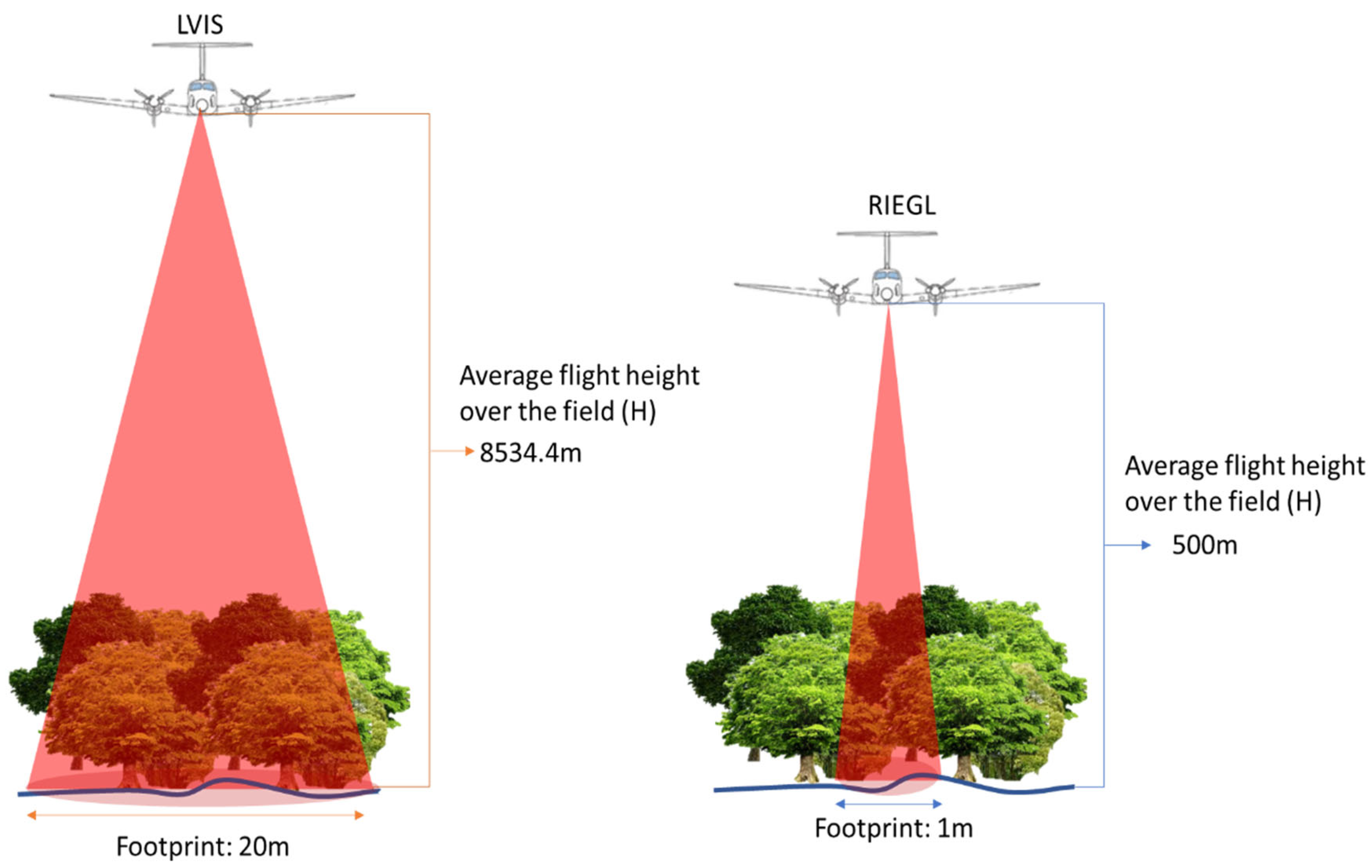
3.1. LVIS Data and RIEGL LMS-Q680i Data

In 2005, the LVIS-equipped King Air B-200 aircraft collected surface reflectance data above the SRNP. The LVIS system captured over 180,000 waveforms decoded from 432 bins for each LiDAR echo beam (

Table 1. Parameters of LVIS and RIEGL LMS-Q680I LiDAR systems.

	Footprint Size	Wavelength	Accuracy	Operating Altitude	Pulse Firing Rate	Operation Date
LVIS	20 m	1064 nm	≤2 m	<10 km	100–500 Hz	1995–present
RIEGL LMS-Q680I	1 m	1550 nm	≤20 mm	1–1.6 km	80k–240 kHz	2008–present

). Under the LVIS Data Structure (LDS) coding, the original binary data were reorganized to LVIS Canopy Elevation (.lce), LVIS Ground Elevation (.lge), and an LVIS Geolocated Waveform (.lgw) formats, respectively.

The second dataset was obtained from the RIEGL LMS-Q680i system. Using a high laser pulse (repetition rate up to 400 kHz) and more than 260,000 measurements per second, the RIEGL LMS-Q680i collects high-quality data independent of the complexity of the terrain (Table 1). In 2021, Stereo Carto Central America provided a 2000 m scan of the SRNP image with 1 m resolution. After image preprocessing and raw LiDAR processing, the *.tif-contained image data and the *.las file-restored point clouds data were used in this study.

In 2005, LVIS undertook a data acquisition mission on several tropical forests, employing 20 m diameter footprints. For the Santa Rosa National Park Environmental Monitoring Super Site, this endeavor was conducted through three tracks, each contributing to the comprehensive coverage of the designated study area. In a parallel yet distinct undertaking, Sterorecarto, in 2021, carried out LiDAR collection activities targeting a subset of SRNP forests using a RIEGL LMS-Q680i, specifically focusing on overlapping areas with the LVIS mission. It is important to highlight that during the 2021 data collection, Stereocarto ensured meticulous error control measures, successfully containing an overall error magnitude within 2 cm.

The LVIS was conducted during the dry season of 2005, a period during which most trees were in a leaf-off stage. This limited tree canopy crown density influenced the energy returned to the sensor, resulting in modifications to the waveform when compared with the leaf-on season data collected using the RIEGL LMS-Q680i. In 2021, the RIEGL LMS-Q680i gathered leaf-on data from TDFs during the wet season. During the leaf-on season, the proliferation of leaves in the TDFs resulted in a greater number of canopy returns. Despite the difference in phenology, all successional stages used in this study were identified in both the 2005 and 2021 data sets since the study has been extensively studied for changes in ecosystem structure and composition since 1998.

3.2. Description of Workflow

In this study, two different types of LiDAR systems were used for the analysis, as indicated above. The workflow used in this study is illustrated in Figure 2. The workflow aims to (1) upscale the small footprints from RIEGL (1 m) to LVIS (20 m), (2) produce the RIEGL waveform and unify its format with the LVIS data, (3) produce the tree waveforms, (4) separate three successional stages, and (5) conduct a comparison using waveform metrics between 2005 and 2021.

This analysis was performed using the LVIS LiDAR 2005 and RIEGL LMS-Q680i 2021 waveforms. The following variables were extracted from the two datasets for 2005 and 2021 (

Table 2. Description of the LiDAR metrics used in this study. WAF is the waveform amplitude-related figure, and NCE is the normalized cumulative return energy-related figure. H_g is the ground return which means elevation of the lowest detected mode within the waveform (m).

Acronym	Source	Unit	Description
RH25	NCE	meter	Relative Height related to $H_g$ at which 25% of the waveform energy occurs.
RH50	NCE	meter	Relative Height related to $H_g$ at which 50% of the waveform energy occurs.
RH75	NCE	meter	Relative Height related to $H_g$ at which 75% of the waveform energy occurs.
RH100	NCE	meter	Relative Height related to $H_g$ at which 100% of the waveform energy occurs.
Cx	WAF	waveform amplitude	The x coordinate of the waveform centroid (under the waveform coordinate system)
Cy	WAF	meter	The y coordinate of the waveform centroid (under the waveform coordinate system)
RG	WAF	null	The second moment of the waveform or the radius of gyration is the root mean square of the sum of the two-dimension distances that all points on the waveform are from its centroid (under the waveform coordinate system)
Annual rate	null	%/year	The annual rate is calculated by the increased value divided by the total years, then divided by the total increased amount. In the thesis, the time period is constant at 16 years.

): Canopy Height (CH) and Relative Waveform Intensity at 25, 50, 75, and 100% of the vertical profile (RH25, RH50, RH75, and RH100), which quantified the vertical changes in vegetation; the visualized balanced point (centroid) of the waveform (Cx and Cy) (Equation (1)), which depicted the changes in waveform amplitude and waveform sensitivity; and the Radio of Gyration (RG), which quantified the changes in waveform shape.

$$C=\frac{\int f\left(x,y\right)\mathrm{d}l}{\int \mathrm{d}l}$$

(1)

It is noticeable that the data collection using the LVIS was conducted during the dry season of 2005, a period during which most trees were in a leaf-off stage. This limited tree canopy crown density influenced the energy returned to the sensor, resulting in modifications to the waveform when compared with the leaf-on season data collected by the RIEGL LMS-Q680i. In 2021, the RIEGL LMS-Q680i gathered leaf-on data from TDFs during the wet season. During the leaf-on season, the proliferation of leaves in the TDFs resulted in a greater number of canopy returns.

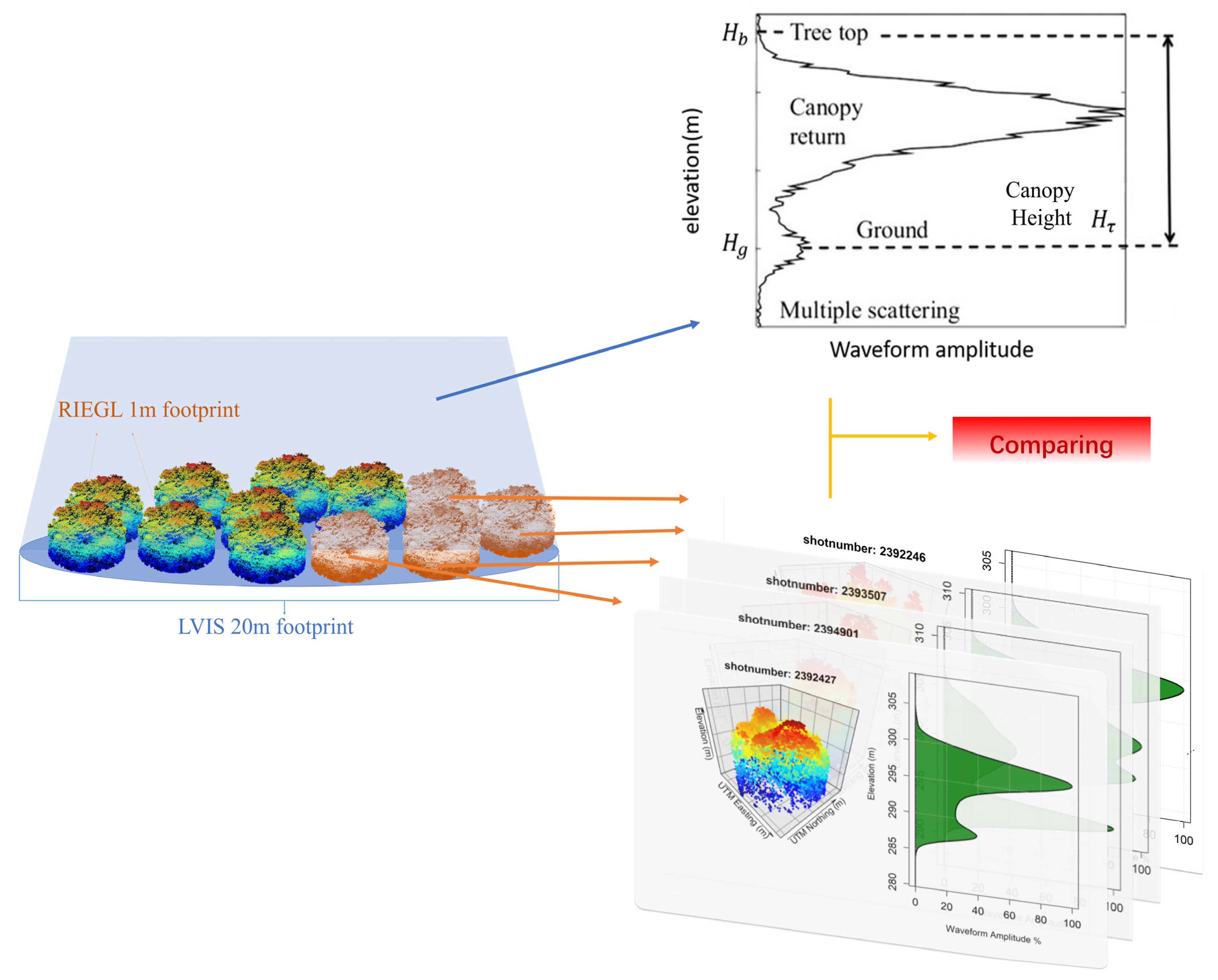
3.3. Pseudo-Waveform Synthesis (RIEGL to LVIS)

To compare forest changes between the two data collections, the smaller footprint (1 m) from the RIEGL system must be upscaled to match the larger footprint (20 m) of the LVIS system (Figure 3). In addition, the formats of the two LiDAR systems should be unified. Hence, several conversions were necessary to match the RIEGL (2021) dataset with the LVIS (2005) dataset.

The “rGEDI” package was utilized to convert “las” files (RIEGL) to “.h5” files (LVIS pre-processing files) to obtain comparable data between the two systems (Figure 4). This process included (1) clipping the RIEGL discrete point cloud within the 20 m LVIS footprint, so a point cloud with a radius corresponding to the LVIS can be produced and (2) using the “rGEDI” package to convert the clipped point cloud to the waveforms with “h5” conversion file. The generated files were classified as “synthesized waveform files”.

Before the process of converting RIEGL data to waveform, a procedure was undertaken wherein the cloud points originated from the RIEGL sensor, so the sampling points were accurately chosen based on the delineation of 20 m circular regions. This procedure involved the RIEGL sampling being centered at the geospatial coordinates of the LVIS (2005) footprints. This selection process harmonized both data sets in terms of their spatial properties.

In addition to the digitized waveforms, the original LVIS files contain additional information, including “zt” and “zg,” which correspond to the elevation of the highest detected return and the lowest detected mode, respectively, as well as the mean signal noise level “sigmean.” After noise cancelation, the LVIS waveform is comparable to the converted RIEGL waveform. By matching data in a comparable format, the same approach can be used to analyze the waveforms.

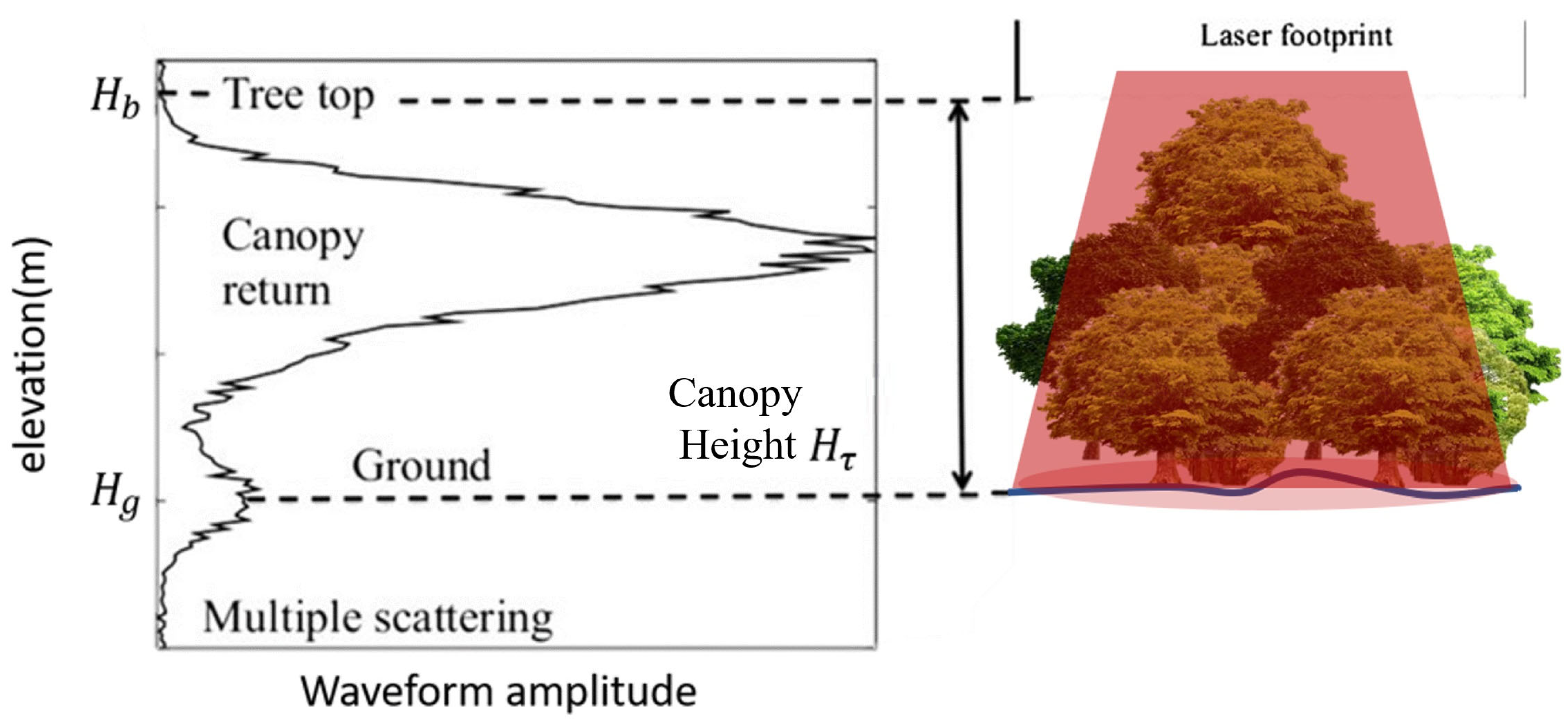
3.3.1. Tree Height from Waveform

Forests are distinguished by the fact that the tree height is determined using waveforms. As the full-waveform LiDAR data shows, the height of the tree is the time elapsed between the treetop returns and the ground returns, which can be determined from the distance between the two most prominent peaks in the amplitude waveform. In the different seasons, TDF exhibits distinct variations in ecosystem which are recorded by the LiDAR waveform. Throughout the wet season, an increased number of leaves reflect energy from the TDF canopy, resulting in waveforms (Figure 5) that display a prominent peak within the primary canopy layer. However, in the dry season TDFs experience a significant reduction in leaf coverage, leading to a decrease in canopy returns and energy absorption compared with the rainy season. Consequently, the dominant peak of the waveforms shifts towards ground returns (Figure 6).

More precisely, the commencement of the signal H_b indicates both the initial return and peak of the canopy (Figure 5 and Figure 6) while H_g indicates the second peak of the returning signal, or the signal reflected off the ground. H_τ represents the total height of the tree.

$$H_{\tau }=H_b-H_g$$

(2)

According to Roberts [25], canopy structure (e.g., density and closure) influences the recognition of the highest point of the canopy instead of the highest peak of the largest mode in a waveform. Therefore, to select the ground peak, Harding et al. [26] specified that the ground surface must be the end-peak of the relative amplitude. They also found that the beginning of the first main peak was at the top of the canopy and the strongest return from the bottom was the ground return. Therefore, it is hypothesized that the RIEGL average tree height ($H_{\tau -RIEGL}$) in 2021 is greater than the LVIS average tree height $H_{\tau -LVIS}$ in 2005.

3.3.2. Waveform Metrics

The most used method for estimating height changes is to calculate the Relative Height (RH) metrics (e.g., RH25, RH50, RH75, and RH100) (Table 2). The vertical heights are denoted as RH25, RH50, RH75, and RH100, based on the vertical distances between the 25%, g50%, 75%, and 100% energy returns. From the LVIS .lge file, the RH metrics are estimated by the function of the zg value, which is the lowest detected elevation within the waveforms. The zg values of the REIGL data may be identified using the same approach, notwithstanding the identical scale waveform amplitude, and ensuring that the RH metrics of the two distinct lidar systems are comparable.

The analysis of waveforms requires shape-based metrics, in addition to RH measurements. According to Muss et al. [27], shape-based metrics present a challenge to the standard energy accumulated approach, specifically in the absence of potential information from the waveform shape and collinearity of the quantile datasets (RH metrics). Using the connection between the shape, location, and wavelength of the LiDAR waveforms, the position of the centroid (Table 2) (C_x and C_y) was computed as a function of the balanced point of the waveforms. The centroid provides more exact and direct information on the position and form of waveforms. In this study, C is relative to the ground, as the detected waveforms indicate that the tree canopy returns to the ground. In addition, the Radius of Gyration (Table 2) (RG) was computed by utilizing the root mean square of the distance between the center of the waveform and its edge to quantify the waveform.

$$RG=\sqrt{\frac{\sum {\left(x_i-C_x\right)}^2+\sum {\left(y_i-C_y\right)}^2}{n}}$$

(3)

3.3.3. Age Group and Succession Stages

Understanding the growth trajectory of secondary forests requires a chronosequence approach, particularly for long-term studies [28]. According to Arroyo-Mora et al. [24], successional phases are influenced by vertical and horizontal structures, the dynamics of leaf flushing (leaf on/leaf off), and the density of the green canopy cover. The four stages of succession include pastures, early succession, intermediate succession, and late succession; since 2005, early forests were still a mixture of pasture and trees, and only the changes that occurred during the intermediate and late succession periods have been considered.

According to Zhao et al. [19], an age-attributed metric can be used to merge LVIS LiDAR data with hyperspectral information to provide an age map with groups of 0–10 years, 10–20 years, 20–30 years, 30–50 years, and 50+ years. Using Zhao et al. [19] as a reference, we considered three forest age groups: 0–30 years (early) old, 30–50 years (intermediate), and >50 years (late). Because there were 16 years between images, the age of the forest also changed. Hence, by 2021, each stage (2005) had moved into the next successional stage: the early to intermediate, the intermediate to late, and late stage remained the same. Then, we separated the late stage in 2021 to late1 and late2. Late1 grew from intermediate stage in 2005 and late2 grew from the late stage in 2005.

4. Results

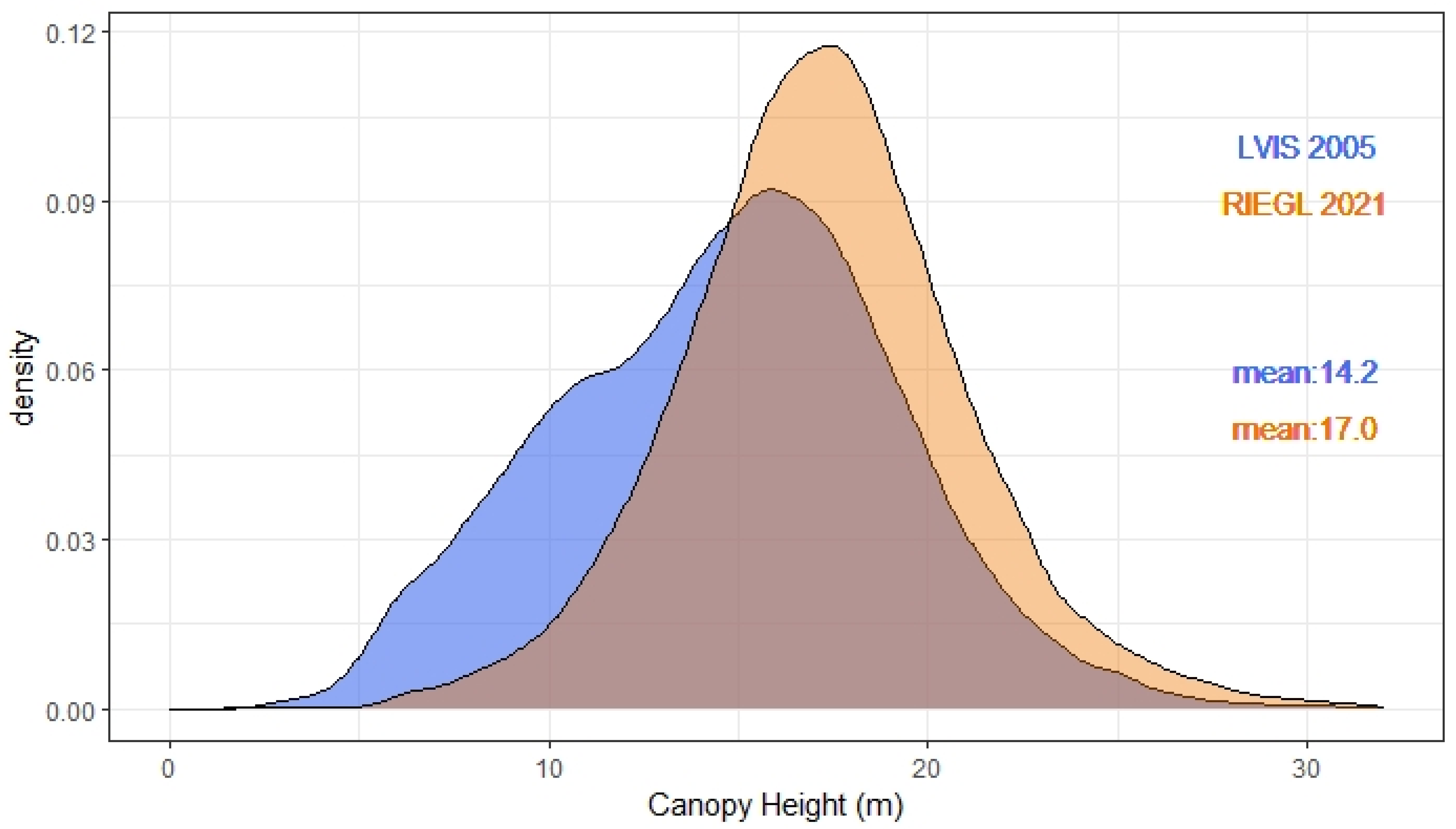
4.1. Change in Relative Height Traits and Canopy Height

Table 3. The 2005 (LVIS) and 2021 (RIEGL) mean Relative Heights with the 25%, 50%, 75%, and 100% energy back with one standard deviation. Data are grouped as a function of successional stages.

Year	2005 (LVIS)			2021 (RIEGL)
Stage	Early	Intermediate	Late	Intermediate	Late1	Late2
RH25 (m)	0.40 ± 0.38	1.25 ± 1.43	2.71 ± 2.39	4.01 ± 2.10	6.15 ± 2.37	8.43 ± 3.34
RH50 (m)	1.32 ± 1.20	4.21 ± 2.82	6.42 ± 3.88	6.25 ± 2.59	9.30 ± 2.74	12.16 ± 3.60
RH75 (m)	3.39 ± 2.06	8.21 ± 3.31	10.11 ± 4.56	8.18 ± 2.83	11.89 ± 2.87	15.13 ± 3.66
RH100 (m)	9.39 ± 3.21	15.49 ± 3.90	17.11 ± 5.91	13.16 ± 3.10	17.52 ± 3.08	21.28 ± 3.92

provides the variations in RH metrics relevant to the four succession stages in 2005 and 2021. The RH25 shows slight fluctuations in height between 2005 and 2021, indicative of the fact that, irrespective of the successional stage, the understory vegetation has increased. In contrast, the alterations in the upper canopy are moderate and increase by two to five meters. The transition from early (2005) to intermediate (2021) has the highest rate of change among the four RH metric groups, about four to ten times that of the other groups. As a comparison of the same age group, late (Table 3) and late1 (Table 3) show similar mean RH75 and RH100 values of 11 m and 17 m, respectively. The trees in the late1 group have already completed the growth transition from intermediate 2005, indicating a high degree of age similarity between the late (2005) and late1 (2021).

Between 2005 and 2021, variations in the mean and standard deviation of the forest’s succession stages are observed, particularly for RH25. During the previous 16 years, the move from the late stage to the late2 stage resulted in an increase of six meters across all RH metric categories (6.3%/year). One conspicuous shift is the marked rise in the RH50 of the early stage in 2005, which surged to 6.25 m by 2021 (6.0%/year), nearly six times its initial height. These findings suggest that tremendous growth and development have transpired within the forest during the specified timeframe. The intermediate to late stages, however, exhibited the least amount of growth over the span of 16 years. This minimal growth is particularly evident in the mere two-meter increase in RH100. It is, nevertheless, important to realize that the changes between the late stage in 2005 and the late1 stage in 2021 are modest for RH75 and RH100, signaling that the forest has stayed generally homogeneous in these higher RH metric categories. In conclusion, it is obvious that the forest has considerably altered in the early stage during the past sixteen years, while remaining rather stable in the late stage.

Figure 7 presents the density distribution of Canopy Heights (CH) in 2005 and 2021. The maximum distributions are observed at 16 and 17 m, respectively. These data are close to the intermediate stage (red) from 15 to 18 m in Figure 8. Nonetheless, there is a substantial variance in CH between 2005 and 2021, with the mean canopy height expanding from 14.2 m to 17.0 m (2.8 m) over the whole study area. Figure 7 also shows that for the CH changes in 2005, there is a distinct gap between the 2021 CH from 0 to 11 m, indicating a transition from pasture to an early successional stage that is not currently observed in the 2005 data.

The intermediate stage (red) in Figure 8 shows CH from the intermediate stage in 2005 to the late1 stage in 2021 for this group. Among the three groups in Table 3 that exhibit a consistent trend in RH100 from the intermediate (2005) to late1 (2021) stages, the trees in this group display the least amount of growth variation.

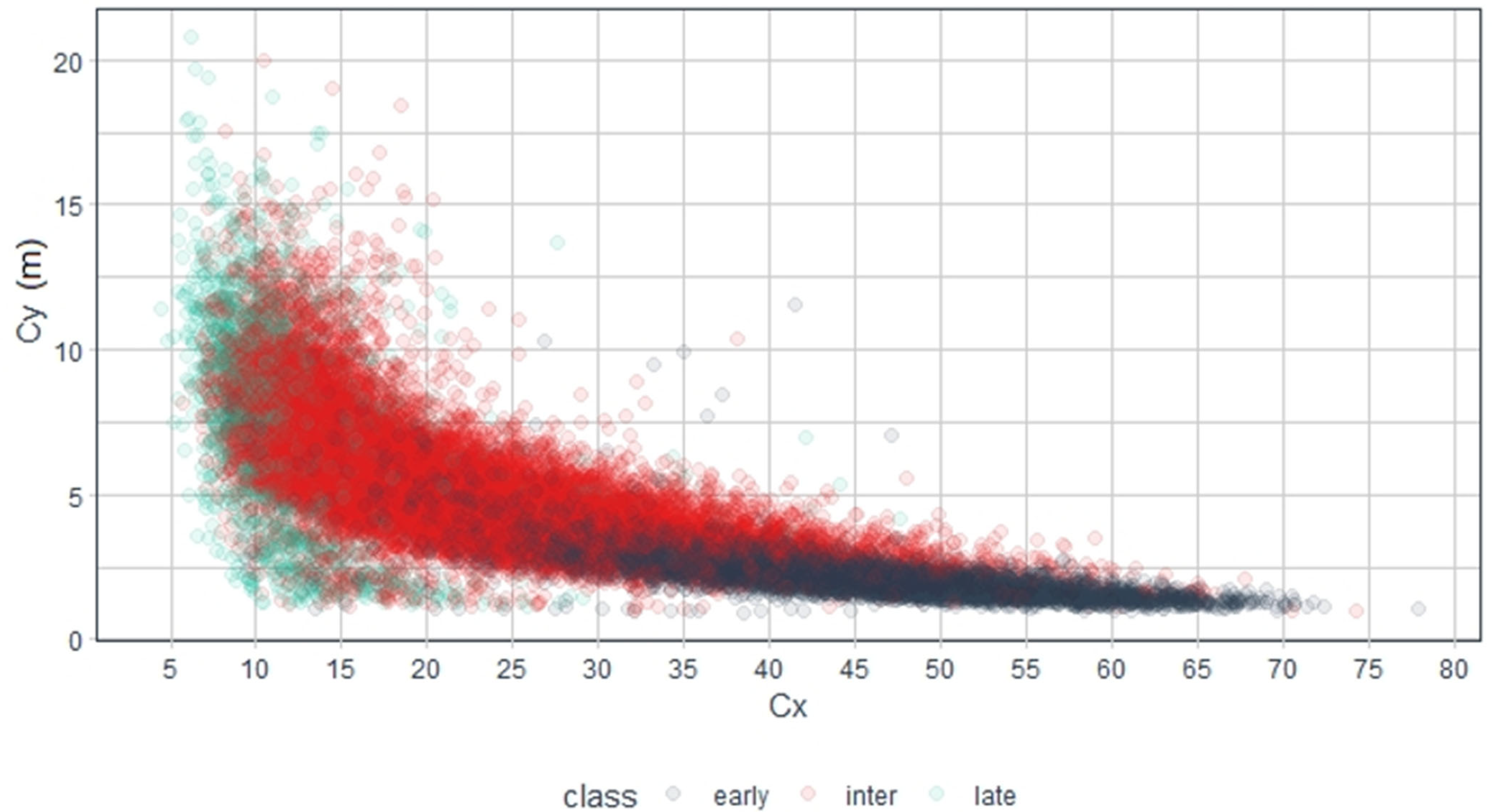
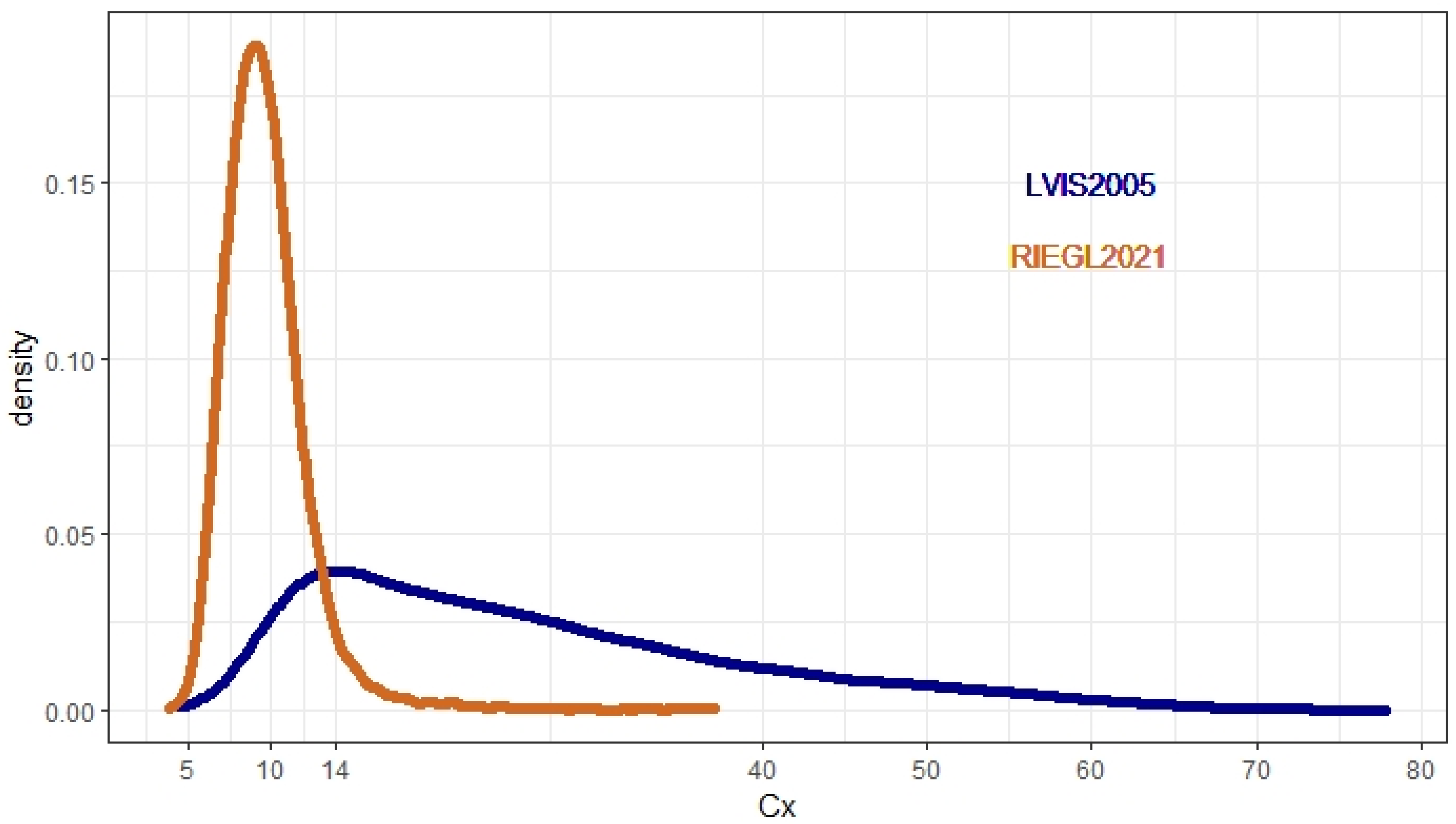
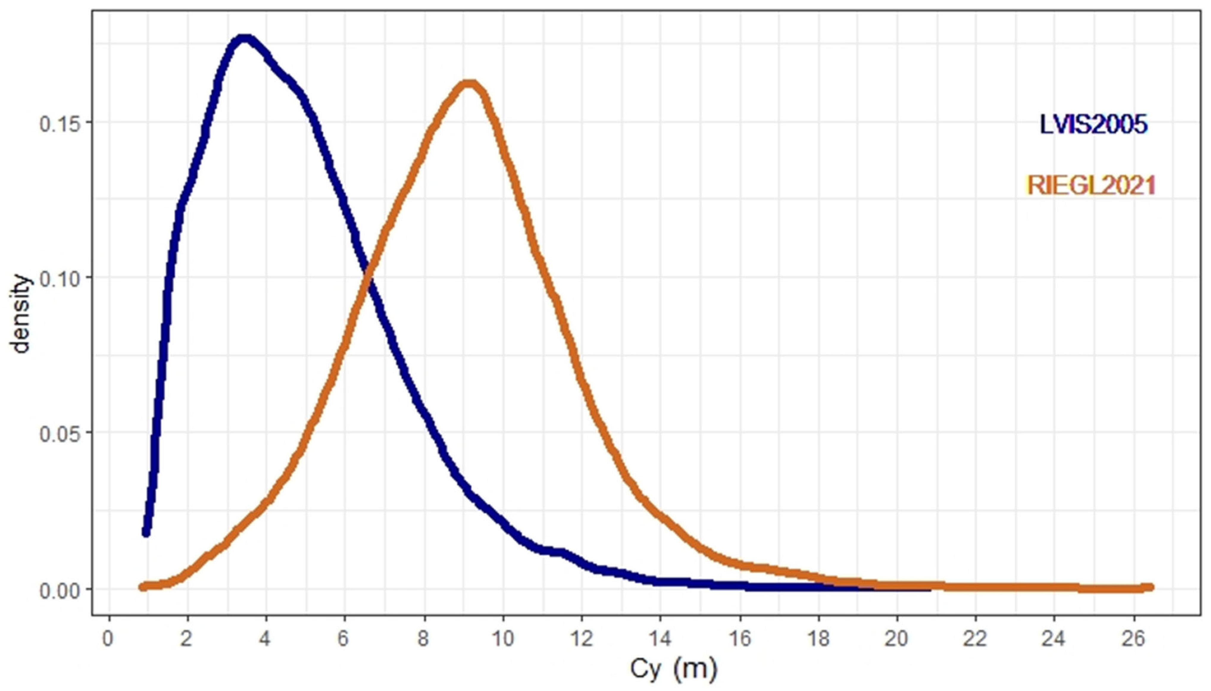
4.2. Comparison of Waveform Centroid Metrics

Figure 9 presents the different Cx and Cy positions of the three successional stages in 2005. The Cx changes between 5 and 20 and the Cy between 10 and 20 m. The intermediate stage follows the late stage, and the Cx in this stage is more adaptable, ranging from 10 to 60. The early stage is depicted at the bottom of the graph with an elevation profile that is approximately 4 m lower. This is because tree height is lower in the early stage, as demonstrated in the RH metrics of Table 3. Moreover, the intermediate stage dominates the graph, which is consistent with the intermediate stage in Figure 8.

In Figure 10, which pertains to the year 2021, the primary Cx values exceed 20, indicating a significant decrease compared with the Cx values in 2005, which is related to the high ground return in leaf-off season. Additionally, the stages are more distinctly separated, with pronounced margins observed between them. The demarcation between the intermediate stage and late1 stages becomes apparent when Cy attains a value of 7, while the distinction between the late1 and late2 stages becomes apparent at a Cy value of 15. Despite some overlap between the late1 and late2 stages, most of the data points are concentrated in the late1 stage.

Furthermore, there is a notable variation in the density of data points among the different growth stages. Specifically, the intermediate stage in 2005 and the late1 stage in 2021 account for most of the points. This trend suggests that the trees have undergone considerable growth, resulting in a denser and more layered canopy.

4.3. Comparing Waveform Line-Shape Based Metrics

In Figure 11, the LVIS (2005) frequency distribution presents a plateau in point density at Cx = 14 and continually decreases the density to Cx = 78. The highest Cx point density in 2021 is reached at a Cx of 9 waveform amplitude. Simultaneously, the max Cx in 2021 reached 37, which is less than half of the maximum value recorded in 2005, which was approximately 78. The 2005 waveform surpasses the 2021 data, suggesting that the ground return energy in 2005 was greater than that collected in 2021. The primary factor driving this difference is that the leaf-off season’s Cx is typically higher than in the leaf-on season. Consequently, less canopy cover is available to absorb the energy during the leaf-off season.

Figure 12 presents a comparison between Cy in 2005 and 2021. The elevation profile is shown by the Y-axis. The data indicate that the 2005 peak is around 3.5 m in height, whereas the 2021 peak is approximately 9 m. The graph depicts a changing trend in the line, which, according to waveform analysis, suggests that the vertical profile is rising since the trees have been growing over a period of 16 years.

Figure 13 presents a comparison for RG between 2005 and 2021. The 2021 density line demonstrates an upward trend as trees are growing, which is expected from an ecological point of view. Figure 13 presents the distribution of RG as a function of successional stage. The tree growth depicted in Figure 14 appears to follow the successional stage group, with the late stage having the highest rate of rise and the highest RG value compared with the early stage in 2005, as indicated by the bottom of the point cloud.

4.4. Comparison of Waveform Centroid Metrics

The correlation between several metrics, including Cx, Cy, RG, CH, and RH100, in both 2005 and 2021 are depicted in Figure 15 and Figure 16. Of these metrics, the relationship between Cx and RG in Figure 15 stands out, as it indicates a high level of correlation. This is because Cx yields a higher value compared with Cy in the calculation of RG, suggesting that ground returns from 2005 are the primary contributor to energy reflectance since the data were collected in the dry season. Additionally, Figure 15 shows that the ground returns during the dry season produced the largest peak, which significantly contributed to the Cx calculation.

Figure 15 also reveals favorable correlations between the CH-RH100, Cy-RH100, and Cy-CH connections. This can be attributable to the fact that variations in CH, Cy, and RH100 are connected to differences in the forest’s vertical profile. In contrast, RG has a negative correlation with CH, RH100, and Cy, indicating that ground returns are very robust and weaken the link between tree height profiles and ground returns.

Moving on to Figure 16, RG is positively influenced by metrics related to vertical profiles, especially in the range of 0.5–1. This is particularly noticeable in the CH-RH100, RG-RH100, and RG-CH relationships, which display the opposite correlation compared with the 2005 data. The reason for this is that during the leaf-on season, multiple canopy layers contribute significantly to energy reflectance, as shown in Figure 5. Consequently, the waveform peak is dominated by canopy reflectance, and the waveform amplitude related to Cx is negatively related to the remaining four metrics.

5. Discussion

This study delves into the topic of waveform metrics and their effectiveness in visualizing the evolution of tropical dry forests (TDFs) in Costa Rica over a period of 16 years. This study uses a combination of LVIS and RIEGL data collected in 2005 and 2021, respectively, to provide a comprehensive analysis of the changes that have occurred in TDFs over time.

In recent years, RIEGL data have been gathered, allowing researchers to study the SRNP in greater detail and at a resolution of 1 m. These data offer valuable insights into the potential changes that may have occurred in TDFs over the past 16 years. By analyzing the waveform metrics from both datasets, the study concluded that tree height and canopy height in the SRNP have increased since the initial LVIS data collection in 2005. This study provides vital information to academics, conservationists, and policymakers concerned with the preservation and management of TDFs. Visualizing the variations in TDFs over time using waveform metrics can help identify areas requiring conservation efforts and project the possible effects of climate change and other environmental variables on these ecosystems. This research contributes to our understanding of TDFs and their significance in tropical environments for sustaining biodiversity and ecological balance.

5.1. Mapping Forest with Time Series by LiDAR

The identification of the different sites under different successional stages was conducted after Zhao et al. [19] using the 2005 LVIS data. The study identified early, intermediate, and late stages for 2005, which were projected to 2021 (16 years later). By 2021, the early stage has become an intermediate stage, the intermediate stage is a late stage, and the late stage has become a young late forest. The former allows us to confidently locate different age groups and stages in the RIEGL 2021 data.

The results of waveform analysis revealed the progressive growth of TDFs at the SRNP. The average canopy height grew by 2.8 m. The ascending variables are also reflected in the rising RH metrics (Table 3), shifting the Cy density position (Figure 12), increasing RG density (Figure 13), and shifting the Cx and Cy positions (Figure 9 and Figure 10). In Figure 7, an interesting gap appears between the 2021 CH line from 0 m to 11 m, which shows that there may be factors contributing to faster growth or development in the early stage compared with the other two successional stages. More related research is required to identify these elements and their possible influence on forest ecosystems.

These findings are consistent with previously published assessments of tropical regions, and our study updates and expands on previous comparisons of canopy height and RH metrics [7]. Moreover, our work updated the comparison to include not only the RH100 height, but also the RH25, RH50, and RH75 heights, along with showing increases in tree heights across all RH matrices. Mora et al. [29] found TDFs showed an increase in tree height in the first 3 years and are expected to continue the growing trend for 15 years. The chronosequence model predicts an increasing trend that matches the results of our work in the RH100 comparison (Table 3) and the Cy changes (Figure 12).

Separately, different successional stages showed different rates of increase. The early stage showed the most significant increase in canopy height, with an increase in approximately 4 m in RH100, whereas the late stage exhibited less growth. Each stage had a unique canopy height range, as demonstrated by Sánchez-Azofeifa et al. [17]. It is noticeable that in Figure 8 and Table 3, the intermediate (2005) to late1 (2021) stages show the least variation in growth. This phenomenon can be attributed to the cross-sectional components of the transition zone between the early to intermediate stages and the intermediate to late stages. In other words, the transition from one stage to the next in this group was relatively smooth and consistent, leading to a more uniform growth pattern and less variation among individual trees.

However, we demonstrated here that the early, intermediate, and late stages result in the uniqueness of Cx, Cy, and RG. Although Figure 12 and Figure 13 show some overlapping point data, the separate distribution of each stage point confirms the sensitivity of the shape-based waveform. However, the study of the successional stage is restricted by the difficulty of continuing data collection, which prevents comprehension of the unique dynamics inside the forest, particularly in the transition zone or the border of the age map [30]. In TDFs, elements such as temperature, humidity, soil moisture, precipitation, and light have a substantial impact on the 16-year growth [31]. Specifically, Nath et al. [31] identified precipitation, temperature, and soil properties as the primary factors affecting secondary forest development. This study utilized long-term data collected between 1988 and 2000, including parameters such as diameter at breast height (DBH), precipitation, temperature, and soil properties. The data revealed a positive correlation between tree growth and both precipitation and soil moisture but a negative correlation between forest growth and temperature. It is critical to recognize that this research does not account for environmental changes that may have occurred in Santa Rosa National Park throughout its 16-year expansion period, since these changes were never documented or examined.

At the same time, the uncertainty (overlay part in Figure 9 and Figure 10) of 2021’s successional stages is the result of the theoretical chronosequence of forest development. Our study showed only one possible trajectory of TDFs growth. However, Borges et al. [32] suggested a possible method to pursue future estimations based on the similarity of forest growth, regardless of the type of forest. Future studies predicting the future development of TDFs should consider the possible relationship between TDFs and other types of forests.

5.2. Seasonal Impact of the TDFs Comparison

The TDFs exhibit a clear differentiation between the wet and dry seasons. During the wet season, the TDFs experience higher levels of soil moisture and precipitation, which leads to an increased flourishing of the forest in comparison with the dry season. In fact, during the wet season, the TDFs exhibit growth patterns like those of wet forests. The growth is slowed, however, and even halted when the dry season arrives [33]. This seasonality is evidenced by the findings from the 2005 LVIS (dry season) and the 2021 RIEGL (wet season) studies. Specifically, the growth of TDFs has been observed to be faster during the wet season compared with the dry season [34].

The seasonality of the TDFs also introduces uncertainty into forest studies, which is manifested in the inverse relationship observed in Figure 15 and Figure 16. The reversal of energy returns in the dry season is because leaves, which are the primary reflectors of LiDAR signals, are absent during this period. Consequently, the LiDAR system detects mostly ground returns rather than canopy returns, resulting in the observed waveform peak (Figure 6). Conversely, during the wet season, when leaves are present on the trees, the LiDAR system detects mostly canopy returns, leading to the observed major energy occupation by canopies.

Simultaneously, early-stage forests comprise a dense herbaceous understory and a massive openness canopy of drought deciduous trees [17]. The results of the 2005 LVIS contain a large number of early-stage forests, as indicated by the lowest canopy height in Figure 7 and Table 3. On the other hand, the intermediate and late stages have a greater number of fast-growing trees, lianas, and evergreen crowns, which offer a thicker canopy to the TDFs in wet season [19]. As a result, the LVIS 2005 early-stage waveform displays a greater number of ground returns than the other two stages in the waveform. Compared with data from 2021, the canopy layers absorb more energy since, presumably, there are no early-stage remnants. The waveform of the 2021 wet season resembles the typical forest LiDAR waveform more closely (Figure 4) [35].

It is worth noting that the seasonality of TDFs introduces some uncertainty into forest studies. As mentioned earlier, the absence of leaves during the dry season can lead to high ground returns and little canopy returns, indicating a lower number of trees or a smaller number of leaves on the trees. This introduces uncertainty into forest studies that rely on LiDAR data, particularly when trying to estimate tree height, tree biomass, and carbon storage. Therefore, it is essential to consider seasonality when using LiDAR data for forest studies, and to take measures to account for the absence of leaves during the different seasons.

Furthermore, it is important to note that the resolution of the original data comparison between LVIS and RIEGL is significantly different, with a ratio of 20:1. This represents a considerable upscaling of the data, which may introduce additional noise and uncertainties into the results. Especially, in 2005 the LVIS data were collected with a lower resolution at the same time with a mean signal noise about 1–2 ms. However, the upscaling approach based on the origin cloud points avoided the noise and errors introduced by the LVIS data. Therefore, the potential impact of this upscaling on the data and the resulting interpretations should also be considered and discussed. The study from Silva et al. [36] pointed out a similar methods to convert the point clouds to waveforms to ensure the small footprint LiDAR system is comparable with large footprints. Silva et al. [36] discovered that the outcomes of the big and small footprints were comparable, particularly the canopy height and ground elevation. And from the preceding paragraph, the SRNP’s TDFs followed a similar pattern of development. As a result of this study, it is advisable that future studies compare data from the same season in order to eliminate the influence of the TDFs’ seasonality, which has no correlation with the footprint size.

6. Conclusions

In this study, the TDFs in Santa Rosa National Park (SRNP) have witnessed growth over 16 years. Based on the Canopy Height, Relative Height, stage group, waveform shape, and line metrics analysis, the following conclusions can be drawn:

• With 16 years of growth, TDFs revealed notable variations in height-related profiles, particularly from RH50-, RH100-, and waveform-produced canopy height. Line- and shape-based waveform metrics recorded all changes in the TDFs during the 16 years of growth. Cy and RG increased during forest growth, and Cy showed a positive relationship, particularly in the 2021 wet season results. Cx is shown to have relatively decreased because the ground returns are lower when the canopy density increases and the canopy height increases.
• Intermediate (2005) and late1 (2021) stage trees contributed to the main canopy height with the largest number of trees. By 2021, it is rare to notice early-stage forests in TDFs using LiDAR.
• The wet and dry seasons in TDFs drive significant changes in the waveform, especially in relation to the Canopy Height and RG. Thus, the same seasonal data introduces fewer influencers in the result, which means that the same season data results are more comparable.

References

1. Marín, G.C.; Nygård, R.; Rivas, B.G.; Oden, P.C. Stand dynamics and basal area change in a tropical dry forest reserve in Nicaragua. For. Ecol. Manag. 2005, 208, 63–75. [Google Scholar] [CrossRef]
2. Siyum, Z.G. Tropical dry forest dynamics in the context of climate change: Syntheses of drivers, gaps, and management perspectives. Ecol. Process. 2020, 9, 25. [Google Scholar] [CrossRef]
3. Kennard, D.K. Secondary Forest succession in a tropical dry forest: Patterns of development across a 50-year chronosequence in lowland Bolivia. J. Trop. Ecol. 2002, 18, 53–66. [Google Scholar] [CrossRef]
4. Li, W.; Cao, S.; Campos-Vargas, C.; Sanchez-Azofeifa, A. Identifying tropical dry forests extent and succession via the use of machine learning techniques. Int. J. Appl. Earth Obs. Geoinf. 2017, 63, 196–205. [Google Scholar] [CrossRef]
5. Castillo-Núñez, M.; Sánchez-Azofeifa, G.A.; Croitoru, A.; Rivard, B.; Calvo-Alvarado, J.; Dubayah, R.O. Delineation of secondary succession mechanisms for tropical dry forests using LiDAR. Remote Sens. Environ. 2011, 115, 2217–2231. [Google Scholar] [CrossRef]
6. Martinuzzi, S.; Gould, W.A.; Vierling, L.A.; Hudak, A.T.; Nelson, R.F.; Evans, J.S. Quantifying Tropical Dry Forest Type and Succession: Substantial Improvement with LiDAR. Biotropica 2013, 45, 135–146. [Google Scholar] [CrossRef]
7. Gu, Z.; Cao, S.; Sanchez-Azofeifa, G.A. Using LiDAR waveform metrics to describe and identify successional stages of tropical dry forests. Int. J. Appl. Earth Obs. Geoinf. 2018, 73, 482–492. [Google Scholar] [CrossRef]
8. Gillespie, T.W.; Saatchi, S.; Pau, S.; Bohlman, S.; Giorgi, A.P.; Lewis, S. Towards quantifying tropical tree species richness in 500 tropical forests. Int. J. Remote Sens. 2009, 30, 1629–1634. [Google Scholar] [CrossRef]
9. Chitale, V.S.; Behera, M.D.; Roy, P.S. Deciphering plant richness using satellite remote sensing: A study from three biodiversity hotspots. Biodivers. Conserv. 2019, 28, 2183–2196. [Google Scholar] [CrossRef]
10. Ghulam, A.; Porton, I.; Freeman, K. Detecting subcanopy invasive plant species in tropical rainforest by integrating optical and microwave (InSAR/PolInSAR) remote sensing data, and a decision tree algorithm. ISPRS J. Photogramm. Remote Sens. 2014, 88, 174–192. [Google Scholar] [CrossRef]
11. Solberg, S.; Hansen, E.H.; Gobakken, T.; Naessset, E.; Zahabu, E. Biomass and InSAR height relationship in a dense tropical forest. Remote Sens. Environ. 2017, 192, 166–175. [Google Scholar] [CrossRef]
12. Castillo, M.; Rivard, B.; Sánchez-Azofeifa, A.; Calvo-Alvarado, J.; Dubayah, R. LIDAR remote sensing for secondary Tropical Dry Forest identification. Remote Sens. Environ. 2012, 121, 132–143. [Google Scholar] [CrossRef]
13. Park, H.; Turner, R.; Lim, S.; Trinder, J.; Moore, D. Analysis of pine tree height estimation using full waveform lidar. In Proceedings of the 34th International Symposium on Remote Sensing of Environment—The GEOSS Era: Towards Operational Environmental Monitoring, Sydney, Australia, 10–15 April 2011; pp. 3–6. [Google Scholar]
14. Schneider, F.D.; Leiterer, R.; Morsdorf, F.; Gastellu-Etchegorry, J.P.; Lauret, N.; Pfeifer, N.; Schaepman, M.E. Simulating imaging spectrometer data: 3D forest modeling based on LiDAR and in situ data. Remote Sens. Environ. 2014, 152, 235–250. [Google Scholar] [CrossRef]
15. Pirotti, F. Analysis of full-waveform LiDAR data for forestry applications: A review of investigations and methods. iForest-Biogeosciences For. 2011, 4, 100–106. [Google Scholar] [CrossRef]
16. Stan, K.; Sanchez-Azofeifa, A. Tropical dry forest diversity, climatic response, and resilience in a changing climate. Forests 2019, 10, 443. [Google Scholar] [CrossRef]
17. Sánchez-Azofeifa, A.; Portillo-Quintero, C.; Durán, S.M. Structural effects of liana presence Structural effects of liana presence in secondary tropical dry forests using ground LiDAR. Biogeosciences Discuss 2015, 12, 17153–17175. [Google Scholar]
18. Janzen, D.H. Costa Rica’s Area de Conservación Guanacaste: A long march to survival through non-damaging biodevelopment. Biodiversity 2000, 1, 7–20. [Google Scholar] [CrossRef]
19. Zhao, G.; Sanchez-Azofeifa, A.; Laakso, K.; Sun, C.; Fei, L. Hyperspectral and Full-Waveform LiDAR Improve Mapping of Tropical Dry Forest’s Successional Stages. Remote Sens. 2021, 13, 3830. [Google Scholar] [CrossRef]
20. Phillips, J.D.; Šamonil, P.; Pawlik, Ł.; Trochta, J.; Danêk, P. Domination of hillslope denudation by tree uprooting in an old-growth forest. Geomorphology 2017, 276, 27–36. [Google Scholar] [CrossRef]
21. Allen, W. Green Phoenix: Restoring the Tropical Forests of Guanacaste, Costa Rica; Oxford Univiversity Press: New York, NY, USA, 2001; p. 310. [Google Scholar]
22. Meléndez Chaverri, C. Viajeros por Guanacaste Microform: [relatos]; Ministerio de Cultura: Juventud y Deportes, Departamento de Publicaciones: San José, Costa Rica, 1974. [Google Scholar]
23. Sánchez-Azofeifa, G.A.; Quesada, M.; Rodríguez, J.P.; Nassar, J.M.; Stoner, K.E.; Castillo, A.; Garvin, T.; Zent, E.L.; Calvo-Alvarado, J.C.; Kalacska, M.E.R.; et al. Research priorities for neotropical dry forests. Biotropica 2005, 37, 477–485. [Google Scholar]
24. Arroyo-Mora, J.P.; Sánchez-Azofeifa, G.A.; Kalacska, M.E.; Rivard, B.; Calvo-Alvarado, J.C.; Janzen, D.H. Secondary Forest detection in a neotropical dry forest landscape using Landsat 7 ETM+ and IKONOS imagery. Biotropica 2005, 37, 497–507. [Google Scholar] [CrossRef]
25. Roberts, D.A.; Nelson, B.W.; Adams, J.B.; Palmer, F. Spectral changes with leaf aging in Amazon caatinga. Trees Struct. Funct. 1998, 12, 315–325. [Google Scholar] [CrossRef]
26. Harding, D.J.; Carabajal, C.C. ICESat waveform measurements of within-footprint topographic relief and vegetation vertical structure. Geophys. Res. Lett. 2005, 32, 1–4. [Google Scholar] [CrossRef]
27. Muss, J.D.; Aguilar-Amuchastegui, N.; Mladenoff, D.J.; Henebry, G.M. Analysis of waveform lidar data using shape-based metrics. IEEE Geosci. Remote Sens. Lett. 2013, 10, 106–110. [Google Scholar] [CrossRef]
28. Quesada, M.; Sanchez-Azofeifa, G.A.; Alvarez-Añorve, M.; Stoner, K.E.; Avila-Cabadilla, L.; Calvo-Alvarado, J.; Castillo, A.; Espírito-Santo, M.M.; Fagundes, M.; Fernandes, G.W.; et al. Succession, and management of tropical dry forests in the Americas: Review and new perspectives. For. Ecol. Manag. 2009, 258, 1014–1024. [Google Scholar] [CrossRef]
29. Mora, F.; Martínez-Ramos, M.; Ibarra-Manríquez, G.; Pérez-Jiménez, A.; Trilleras, J.; Balvanera, P. Testing Chronosequences through Dynamic Approaches: Time and Site Effects on Tropical Dry Forest Succession. Biotropica 2015, 47, 38–48. [Google Scholar] [CrossRef]
30. Duan, M.; Bax, C.; Laakso, K.; Mashhadi, N.; Mattie, N.; Sanchez-Azofeifa, A. Characterizing Transitions between Successional Stages in a Tropical Dry Forest Using LiDAR Techniques. Remote Sens. 2023, 15, 479. [Google Scholar] [CrossRef]
31. Nath, C.D.; Dattaraja, H.S.; Suresh, H.S.; Joshi, N.V.; Sukumar, R. Patterns of tree growth in relation to environmental variabilityin the tropical dry deciduous forest at Mudumalai, southern India. J. Biosci. 2006, 31, 651–669. [Google Scholar] [CrossRef]
32. Borges, S.L.; Ferreira, M.C.; Walter, B.M.T.; dos Santos, A.C.; Scariot, A.O.; Schmidt, I.B. Secondary succession in swamp gallery forests along 65 fallow years after shifting cultivation. For. Ecol. Manag. 2023, 529, 120671. [Google Scholar] [CrossRef]
33. Vieira, D.L.M.; Scariot, A. Principles of natural regeneration of tropical dry forests for restoration. Restor. Ecol. 2006, 55314, 11–20. [Google Scholar] [CrossRef]
34. Poorter, L.; Rozendaal, D.M.; Bongers, F.; de Almeida-Cortez, J.S.; Almeyda Zambrano, A.M.; Álvarez, F.S.; Andrade, J.L.; Villa, L.F.A.; Balvanera, P.; Becknell, J.M.; et al. Wet and dry tropical forests show opposite successional pathways in wood density but converge over time. Nat. Ecol. Evol. 2019, 3, 928–934. [Google Scholar] [CrossRef] [PubMed]
35. Reitberger, J.; Krzystek, P.; Stilla, U. Analysis of full waveform LIDAR data for the classification of deciduous and coniferous trees. Int. J. Remote Sens. 2008, 29, 1407–1431. [Google Scholar] [CrossRef]
36. Silva, C.A.; Saatchi, S.; Garcia, M.; Labriere, N.; Klauberg, C.; Ferraz, A.; Meyer, V.; Jeffery, K.J.; Abernethy, K.; White, L.; et al. Comparison of Small- and Large-Footprint Lidar Characterization of Tropical Forest Aboveground Structure and Biomass:A Case Study From Central Gabon. IEEE J. Sel. Top. Appl. Earth Obs. Remote Sens. 2018, 11, 3512–3526. [Google Scholar] [CrossRef]
Figure 1. Location of the Santa Rosa National Park Environmental Monitoring Super Site in Guanacaste, Costa Rica, and the footprint of the LVIS data and the RIEGL LMS-Q680i data used in this study. The color ramp in LVIS, ranging from blue to yellow, represents the elevation changes from low to high. In the RIEGL LMS-Q680i system, a color gradient from dark red to white signifies a similar shift in elevation, with low elevations represented by lighter colors and higher elevations by darker shades. Base map source: ESRI Satellite, http://server.arcgisonlie.com/ArcGIS/rest/services/World_Imagery (accessed on September 3 2023) and ESRI National Geographic, http://services.arcgisonline.com/ArcGIS/rest/services/NatGEO_World_Map (accessed on 1 September 2023).
Remotesensing 15 04677 g001
Figure 2. Workflow applied to the LVIS and RIEGL datasets to analyze changes in forest structure as a function of successional stage between 2005 and 2021.
Remotesensing 15 04677 g002
Figure 3. LVIS footprints are recorded with a footprint diameter of 20 m for the 2005 flight. The RIEGL system used a 1 m footprint to derive a discrete point cloud from the waveform information in 2021.
Remotesensing 15 04677 g003
Figure 4. Workflow associated with the processing of the waveforms: (1) The LVIS centroids were located; (2) The discrete point cloud is clipped using the standard LVIS radius; (3) The .h5 files are derived from all those individual point clouds. Then, we compared the LVIS (2005) waveform and the .h5 waveform from RIEGL (2022).
Remotesensing 15 04677 g004
Figure 5. The treetop is the first return represented by Hb, the main ground return is represented by Hg, and Hτ is the tree height during the wet season. During the wet season, more leaves return the energy from the tree top and waveform showing the dominant peak in the main canopy. During the wet season, more leaves return energy from the tree top and waveform, showing a dominant peak in the main canopy.
Remotesensing 15 04677 g005
Figure 6. The left figure represents a waveform from the dry season. During this time of year, the TDF’s leaves drop substantially, the canopy returns, and the energy absorption is lower than during the rainy season. The ground returns from the dominant crest of the waveforms.
Remotesensing 15 04677 g006
Figure 7. Density chart showing the density of Canopy Heights (CH) in 2005 and 2021. Blue represents the LVIS 2005, and orange represents RIEGL 2021.
Remotesensing 15 04677 g007
Figure 8. Point graph showing the different Canopy Heights (CH) for the early, intermediate, and late successional stages in 2005, and then changes to the intermediate, late1, and late2 stages in 2021. Curved circles represent the density. When circle size increases, a lower density is represented.
Remotesensing 15 04677 g008
Figure 9. Point graph showing Cx and Cy as representing each footprint’s centroid of the 2005 waveforms. Separated colors express the early stage in dark, intermediate stage in red, and the late stage in blue.
Remotesensing 15 04677 g009
Figure 10. Point graph using Cx and Cy to represent each footprint’s centroid of the 2021 waveform. Separated color express the intermediate stage in dark, the late1 stage in red and the late2 stage in blue.
Remotesensing 15 04677 g010
Figure 11. Frequency distribution of Cx illustration changes between 2005 and 2021.
Remotesensing 15 04677 g011
Figure 12. Frequency distribution of Cy illustration changes between 2005 and 2021.
Remotesensing 15 04677 g012
Figure 13. Line graph illustrating the density of the RG distribution in 2005 and 2021.
Remotesensing 15 04677 g013
Figure 14. Point graph showing the RG points grouped by the early, intermediate, and late stages. The X axis represents the LVIS 2005 data, and the Y axis is RIEGL 2021 data. The colors black, red, and blue represent the early stage, intermediate stage, and late stage, respectively.
Remotesensing 15 04677 g014
Figure 15. Correlation graph showing the relation between the Cx, Cy, RG, CH, and RH100 metrics in 2005. The color gradient represents the degree of positivity or negativity between the measurements. Blue is negative, whereas red is positive.
Remotesensing 15 04677 g015
Figure 16. Correlation graph showing the relation between the Cx, Cy, RG, CH, and RH100 metrics in 2021. The color gradient represents the degree of positivity or negativity between the measurements. Blue is negative, whereas red is positive.
Remotesensing 15 04677 g016