Estimating the Quality of the Most Popular Machine Learning Algorithms for Landslide Susceptibility Mapping in 2018 Mw 7.5 Palu Earthquake

Abstract

The Mw 7.5 Palu earthquake that occurred on 28 September 2018 (UTC 10:02) on Sulawesi Island, Indonesia, triggered approximately 15,600 landslides, causing about 4000 fatalities and widespread destruction. The primary objective of this study is to perform landslide susceptibility mapping (LSM) associated with this event and assess the performance of the most widely used machine learning algorithms of logistic regression (LR) and random forest (RF). Eight controlling factors were considered, including elevation, hillslope gradient, aspect, relief, distance to rivers, peak ground velocity (PGV), peak ground acceleration (PGA), and lithology. To evaluate model uncertainty, training samples were randomly selected and used to establish the models 20 times, resulting in 20 susceptibility maps for different models. The quality of the landslide susceptibility maps was evaluated using several metrics, including the mean landslide susceptibility index (LSI), modelling uncertainty, and predictive accuracy. The results demonstrate that both models effectively capture the actual distribution of landslides, with areas exhibiting high LSI predominantly concentrated on both sides of the seismogenic fault. The RF model exhibits less sensitivity to changes in training samples, whereas the LR model displays significant variation in LSI with sample changes. Overall, both models demonstrate satisfactory performance; however, the RF model exhibits superior predictive capability compared to the LR model.

1. Introduction

Strong earthquakes frequently give rise to numerous seismic landslides in mountainous areas, resulting in significant casualties and extensive property losses. Consequently, these catastrophes further exacerbate the risk of earthquakes [1,2,3]. Over the past few decades, earthquake-induced landslides have garnered considerable attention, with primarily focus on the development of landslide databases [4,5], analysis of distribution patterns [6,7,8], assessment of susceptibility and hazards [9,10,11,12], and exploration of landscape evolution [13,14,15]. Among them, LSM assumes paramount importance, as it plays a pivotal role in emergency response, facilitating effective disaster recovery, and aiding in reconstruction efforts [9,16,17,18].

Currently, the most commonly employed methods for assessing coseismic landslide susceptibility include data-driven machine learning methods [5,16,19] and the Newmark method based on mechanics mechanisms [20,21]. The physically-based Newmark method comprehensively considers the occurrence mechanism of earthquake-induced landslides and utilizes slope instability outcomes and seismic displacement to quantitatively categorize the susceptibility level of coseismic landslides [22]. It has emerged as a widely utilized approach for susceptibility assessment of seismic landslides worldwide [23,24]. This method has been successfully applied in coseismic landslides of different quake events in various regions, such as the 1994 Mw 6.7 Northridge earthquake [25], 2008 Mw 7.9 Wenchuan earthquake [26], 2013 Mw 6.7 Lushan earthquake [27], 2014 Mw 6.1 Ludian earthquake [28], 2015 Mw 7.9 Nepal earthquake [29], 2017 Mw 7.0 Jiuzhaigou earthquake [30], and 2017 Mw 6.9 Milin earthquake [31]. However, the Newmark model for coseismic landslides requires multiple parameters, including terrain characteristics, geotechnical mechanics, groundwater conditions, and seismic motion. Due to existing limitations, obtaining accurate rock and soil parameters, as well as precise seismic motion distribution across large areas, remains challenging [23,27]. Consequently, there exists a discernible gap between the acquired parameters and the actual input data. As a result, the current regional landslide evaluation outcomes using the Newmark model are not optimal [32].

The landslide susceptibility assessment using data-driven models assumes that, within a certain area, the influencing factors of past landslides will also lead to future landslides [19,33]. These algorithms construct assessment models by analyzing the correlation between causative factors and the distribution of past landslide occurrences [34,35,36]. These models primarily include statistical and machine learning algorithms, such as logistic regression (LR) [16], artificial neural network (ANN) [37], support vector machine (SVM) [38], decision tree (DT) [39], and others. Particularly, in recent years, with the advancements in GIS and machine learning technology, these algorithms have gained widespread usage in LSM. Some studies have employed different algorithms for LSM and compared the prediction ability and accuracy of these models. At present, LR is widely used for nonlinear multivariate statistical modeling in landslide susceptibility assessment due to its advantages of simple calculations and clear physical interpretation [17,35]. However, LR is constrained by normalcy and linearity assumptions. As a linear model, it performs poorly when dealing with non-linear issues or several affecting elements [40]. Recently, more advanced machine learning techniques such as random forest (RF) [40], XGBoost [41], and convolutional neural network (CNN) [42] have been employed for LSM. These models exhibit superior performance in capturing non-linear relationships among influencing factors when compared to the LR model. This enhanced capability leads to improved applications and increased predictive accuracy in regional landslide susceptibility evaluation. Specifically, multiple studies have demonstrated that random forest (RF) outperforms other models in susceptibility mapping [40,43].

On 28 September 2018, a large and shallow earthquake occurred in the Minahasa Peninsula, Indonesia, with its epicenter located at 0.178°S, 119.840°E. This seismic event is notable as the deadliest earthquake to strike Indonesia since the Yogyakarta earthquake in 2006. Furthermore, it was also the most fatal earthquake globally in 2018. The catastrophe resulted in a tragic loss of life, with a reported death toll of at least 4340 people, while over 10,000 individuals sustained injuries, with 4612 being severely injured. Furthermore, the earthquake caused extensive damage to more than 70,000 houses, leaving tens of thousands of people displaced and seeking shelter in temporary accommodations and tents. However, to our knowledge, no relevant LSM of this event has been studied in detail since the earthquake’s occurrence. Meanwhile, there is no general agreement on the procedures or range for LSM, and the application of RF as the most popular machine learning algorithm in earthquake-induced landslide susceptibility is limited. Thus, this study aims at LSM associated with the 2018 Palu earthquake for estimating the quality of the most popular machine learning algorithms of LR and RF models. We investigate LSM for the Palu earthquake by applying and comparing these two methods. Eight causative factors were considered using for modelling, and the landslide mappings were tested by the Receiver Operating Characteristic (ROC) curve and statistical measures. Finally, we quantitatively evaluate the susceptibility maps of the two models based on their modeling process and prediction accuracy. The main objective of this study is to precisely estimate and map landslide susceptibility in the Palu region. This endeavor will serve as a crucial foundation for land use planning, prioritizing evacuation strategies, and executing effective mitigation measures within the area.

2. Geological Setting and Landslide Inventory of Palu Earthquake

2.1. Geological Setting

Central Sulawesi is situated at a geologically intricate intersection of the Philippine Sea, Australian, Sunderland, and Pacifica plates [44,45,46]. Sulawesi is primarily influenced by the Palu-Koro (PK) fault, which is an active left-lateral strike slip fault trending NNW–SSE [47]. The Mw 7.5 Palu earthquake occurred within the PK fault zone [48]. The epicenter of the earthquake is situated approximately 80 km north of Palu city at coordinates 0.178°S, 119.840°E. According to USGS seismic data, around 50 aftershocks were recorded until September 30 (Figure 1). The study area demonstrates significant topographic relief, with elevations ranging from −6 m to 2800 m. On average, the elevation is approximately 1500 m (Figure 1). The lithology of the study area primarily consists of sedimentary rocks spanning the Holocene to Upper Cretaceous periods, as well as Miocene volcanic rocks such as granite and diorite, alongside Cretaceous–Palaeogene and Triassic metamorphic rocks [49]. The study area is situated in close proximity to the equatorial zone, thereby exhibiting a characteristic tropical rainforest climate, specifically identified as a humid subtropical monsoon climate. It boasts an extensive expanse of tropical rainforests. The area sustains consistently elevated temperatures and substantial precipitation throughout the year, with an annual average rainfall exceeding 2500 mm.

2.2. Landslide Inventory of the Palu Earthquake

According to earthquake reports, this devastating earthquake resulted in over 2000 fatalities, displacing 206,494 individuals. The estimated property losses amount to a staggering USD 911 million, while the projected costs for rehabilitation and reconstruction are estimated at a substantial USD 1.5 billion [50,51]. Based on post-quake images with pre-quake images of the Google Earth (GE) platform, whose acquisition dates for images range from two to three months before and after the earthquake, and using 3 m Planet images to reinvestigate the cloud-coverage area, the seismic landslides were detected within the quake-affected area by visual interpretation method [4]. The result shows that the 2018 Palu earthquake triggered a total of approximately 15,700 coseismic landslides across a region spanning 14,600 km². The landslides observed in this study predominantly comprise shallow landslides, along with a smaller number of large-scale liquefaction-induced flowslides, debris flows, and rockslides. The majority of these landslides are distributed within the peak ground acceleration (PGA) range of 0.3 g (Figure 2). The total area affected by seismic landslides was approximately 43.0 km², with an average area of 2700 m². Notably, the Petobo landslide stood out as the largest, covering an extensive area of approximately 1.97 km², while the smallest landslide measured as little as 45 m² (Figure 2). The majority of landslides fell within the range of 500–2500 m², constituting around 60% of the total amount (Figure 2). Moreover, 414 landslides encompassed an individual area exceeding 10,000 m², and a total of 1393 landslides are greater than 5000 m² [4]. The results indicate that the coseismic landslides are primarily influenced by the seismogenic fault. Furthermore, landslides exhibit a strong correlation with several factors, including elevation, slope angle, aspect, rock type, and peak ground acceleration (PGA). Landslide occurrence increases with greater slope angles, PGA, and topographic relief [4].

3. Data and Methods

3.1. Data Sources

In statistical methodologies, independent variables encompass various factors that exert control the landslide occurrences, primarily encompassing geological, topographical, and seismic factors [34,52]. In this study, eight influencing factors were used for modelling including elevation, hillslope gradient, aspect, topographic relief, distance to the rivers, Peak Ground Acceleration (PGA), Peak Ground Velocity (PGV), and lithology. The elevation data are derived from DEMNAS DEM data with 8 m resolution from the Indonesian Geospatial Information Agency [53]. The information of hillslope gradient and aspect are calculated by these elevation data. Meanwhile, we estimate the relief from the altitude range within a 2.5 km radius [2]. For lithological data, we digitize the Sulawesi geological map with 1:250,000 scale from Leeuwen and Muhardjo [54] and Watkinson [49] to obtain the lithological information of the study area. The rivers are derived from the elevation data, and the distances from the centroid of the cells to the nearest drainages are determined using ArcGIS. Additionally, PGA and PGV information is collected from the United States Geological Survey (USGS) [55]. Based on the PGA distribution provided by USGS, the maximum PGA value is 0.9 g, while the minimum value within the study area is 0.2 g. High PGA values are predominantly observed on both sides of the seismogenic fault. Similarly, the distribution of PGV follows the pattern of PGA, with PGV decreasing rapidly as the distance from the seismogenic fault increases. The maximum PGV value is 108 m/s, while the minimum PGV value is 8 m/s. The lithological map reveals that the Permo-Triassic metamorphic rocks (Pc) and Middle Miocene sedimentary rocks (Mm) cover the largest proportions, constituting 23.5% and 18.6% of the total area, respectively. In contrast, Miocene volcanic rocks (Mv) have the smallest coverage area, representing only 0.8% of the total area. Finally, eight factors are considered for the modeling process. The maps representing these eight influencing factors are transformed into a raster format using a cell size of 8 m (Figure 3).

3.2. Method

The logistic regression (LR) model is a multivariate statistical method extensively utilized in landslide susceptibility analyses [56]. At present, various statistical techniques, including the LR model, weight of evidence, SVM, and CNN can be employed for assessing landslide susceptibility. However, among these methods, the LR model is widely recommended for conducting landslide susceptibility assessments [35,57]. Meanwhile, it is also the preferred method for establishing the near-real-time model of coseismic landslides [52,58,59]. The LR model provides a relative estimation of earthquake-induced landslide occurrence by incorporating various factors. It utilizes maximum likelihood estimation and converts dependent variables into binary logical variables, where “1” represents the presence of landslides and “0” represents their absence [33,56]. This approach effectively addresses the interdependence among factors and offers a comprehensive solution. The correlation between the probability of landslide occurrence and these factors can be expressed as follows:

$$\mathrm{Z}={\mathsf{\beta }}_0+{\mathsf{\beta }}_1{\mathsf{\chi }}_1+{\mathsf{\beta }}_2{\mathsf{\chi }}_2+{\mathsf{\beta }}_3{\mathsf{\chi }}_3\dots {\mathsf{\beta }}_{\mathrm{i}}{\mathsf{\chi }}_{\mathrm{i}}$$

(1)

$$\mathrm{P}=1/(1+{\mathrm{e}}^{-\mathrm{z}})$$

(2)

where $\mathrm{P}$ is the predicted probability of the coseismic landslide; ${\mathsf{\chi }}_1,{\mathsf{\chi }}_2\dots {\mathsf{\chi }}_{\mathrm{i}}$ are the influencing factors; and ${\mathsf{\beta }}_0,{\mathsf{\beta }}_1\dots {\mathsf{\beta }}_{\mathrm{i}}$, are the regression coefficients determined in LR model.

The random forest (RF) model is a powerful ensemble-learning algorithm which was proposed by Breiman [60]. It is a non-parametric method and widely recognized for its flexibility in assessing complex connections between variables for determining landslide susceptibility [40]. This algorithm employs bootstrap sampling techniques on the training samples, allowing it to select a subset of independent variables at each node. Due to its versatility, RF has gained popularity across various fields and has consistently demonstrated exceptional performance [61,62]. The RF model is built upon the concept of bootstrap aggregation (bagging) and incorporates two random sampling techniques, enhancing both the stability and the accuracy of the model. This approach also mitigates sensitivity to outliers and noise while effectively addressing the issue of overfitting [63]. The RF model also offers a number of metrics of variable relevance, with the most accurate one coming from evaluating the drop in classification accuracy when a variable’s values are randomly permuted within a tree node. Unlike other models, RF’s assessment ensures robust evaluation and reliable determination of variable importance. The output of RF is determined by a voting process, shown in Equation (3).

$$\mathrm{H}\left(x\right)={arg}_z^{max}{\sum }_{i=1}^{k}I(h_i\left(x\right)=Z)$$

(3)

$\mathrm{H}\left(x\right)$ denotes the RF model. $h_i$ is a single decision tree model, Z is the output variable, and $I(h_i\left(x\right)=Z)$ is the indicative function.

The correlation coefficients of the influencing factors were estimated by the Pearson method, which is commonly employed for assessing relationships between continuous variables [52,64]. When examining the correlation matrix, a high correlation coefficient (>0.7) between two variables indicates a strong pairwise collinearity [58,64]. In such cases, it is necessary to discard one of the two factors to avoid redundancy. We assessed the correlations among all the relevant factors, with the exception of lithology (Figure 4), because the Pearson correlation coefficient requires both variables to be continuous. The results show that PGA and PGV have the greatest association, reaching 0.9. Therefore, in the modeling process, we only selected PGA for susceptibility assessment without PGV. The hillslope gradient and relief come in second, with a correlation coefficient of 0.67, and there is little relationship between the remaining factors.

4. Results

In order to compare the impact of different training samples on the assessment model and evaluate the uncertainty of the model, this study randomly selected landsliding and non-landsliding samples to establish the assessment model 20 times. We randomly selected 15,600 points within the landslide area as landsliding samples. For the selection of non-sliding samples, we randomly selected 15,600 non-sliding samples in non-landslide areas. Finally, 20 sets of modeling samples were trained by the LR model to obtain 20 predicted pictures of potential landsliding. Figure 5 shows the average and standard deviation distribution of different susceptibility results obtained from 20 different LR models. The results show that the susceptibility map obtained by the LR model can better reflect the actual distribution of landslides, with areas with higher susceptibility index (LSI) mainly concentrated along both sides of the seismogenic fault. The areas with high LSI mainly include the southern part of the epicenter and the areas on both sides of the Palu basin, which are also the landslide abundance areas. Figure 5b shows the standard deviation (std) distribution of 20 prediction results for different training sample scenarios. From the predicted results, we can observe that, for the LR model, the maximum std and minimum std of the modelling results are 0.4 and 0, respectively. Based on the same sampling method, we trained 20 sets of modeling samples using the RF model to obtain 20 LSI maps. Figure 6 shows the distribution of average value and std of different LSM obtained by different 20 RF models. The results show that the RF model can also predict the location of landslide prone areas well. The landslide abundance area roughly matches the area of high LSI, and most landslides are located in the blue area, that is, the area with high LSI. Figure 6b shows the std distribution of 20 prediction results for different training sample scenarios. Compared to the LR model, the std of the RF model is smaller, with a max std of 0.13.

Figure 7 shows the scatter plots of the average LSI and std values under two different models. The statistical results show that the average LSI and std of the two models show the same trend. As the LSI increases, the std shows a trend of rising and then decreasing, with the areas with larger std concentrated in the LSI values of 0.3–0.7. This indicates that the predicted areas with an average LSI between 0.3 and 0.7 are greatly influenced by the changes in training samples, and the std is roughly distributed between 0.04 and 0.1. In contrast, the predicted areas with an average LSI of less 0.3 and larger 0.7 are less affected by the training samples, and the overall std is less than 0.04. In addition, from the values of the std for the two models, the std based on the RF model is lower than that of the LR model, indicating that the evaluation results using the RF model are less affected by the changes in training samples, while the predicted result of the LR model has a relatively large variation in LSI with the changes in training samples.

Figure 8 illustrates the frequency density distribution of the LSI under the two susceptibility models. The results reveal a notable disparity in the frequency distribution of LSI between the two models. For the LR model, the LSI is primarily distributed within the range of 0.1 to 0.5, representing 52.9% of the total grid count. Interestingly, the number of grids with LSI values below 0.1 and above 0.5 is roughly equal, accounting for 23.3% and 23.8% of the total number, respectively. Conversely, the RF model exhibits a higher proportion of grids with LSI values below 0.1, constituting nearly half of the total number. Moreover, the number of grids falling within the LSI range of 0.1 to 0.5 predicted by the RF model is smaller compared to the LR model, accounting for 35.6%. Similarly, the RF model predicts fewer grids with LSI exceeding 0.5 in comparison to the LR model, amounting to 15.8% of the total grid count within this range.

The landslide susceptibility map can be classified into very low susceptibility areas (<0.1), low susceptibility areas (0.1–0.3), medium susceptibility areas (0.3–0.5), high susceptibility areas (0.5–0.7), and extremely high susceptibility areas (0.75–1) based on the LSI values, and we can obtain the landslide susceptibility classification maps of two models (Figure 9). In order to compare the susceptibility results of different models, we calculate on the landslide areal density (LAD) within different susceptibility zones. Figure 10 illustrates the susceptibility classification results and landslide area density (LAD) predicted by the different models. The result shows that approximately 60% of the study area is classified as very low susceptibility or low susceptibility in both models. Specifically, the LR model predicts a very low susceptibility area accounting for 25% of the total area, while the RF model predicts a larger very low susceptibility area, covering 49% of the total area. For the extremely high susceptibility area, i.e., the red area, the predicted area by the LR model and the RF model accounts for 11% and 8% of the study area, respectively. Overall, the two models exhibit similar predictions for medium, high, and extremely high susceptibility areas. However, there are significant differences in the predicted areas for extremely low and low susceptibility. Furthermore, the LAD curves plotted for different intervals indicate a consistent increasing trend with the rise of the landslide susceptibility index (LSI). However, the trend is more pronounced in the RF model due to its higher prediction of landslides in the extremely high susceptibility area. In the extremely high-susceptibility area, RF predicted over 76% of landslides in 8% of the study area, while LR predicted 57% of the total landslide area in 11% of area.

The ROC curve is utilized to assess the accuracy of the modelling, as described by [65]. The AUC (Area Under the Curve) is a measure of the model’s predictive capability. An AUC value of 0.5 indicates a stochastic model, while an AUC between 0.5 and 0.7 suggests lower accuracy. On the other hand, an AUC between 0.7 and 0.9 indicates high accuracy, as stated by [66]. By comparing the assessment results with the actual landslides, ROC curves were generated (Figure 11). The results show that both models have high prediction accuracy, reaching above 0.85. The LR model yields AUC values ranging from 0.85 to 0.86, indicating moderate prediction ability. In contrast, the RF model demonstrates slightly superior performance, with AUC values ranging between 0.92 and 0.94. Overall, these results indicate that the RF model exhibits higher prediction accuracy compared to the LR model.

In order to quantitatively test the correlation between the average LSI of the two models, we randomly selected 15,600 sampling points within the study area to analyze the correlation between the LSI values of the two models. Figure 12 shows the scatter plot of the average LSI values under two different models. The result shows that the two models show a linear relationship of ${LSI}_{RF}=0.75\ast {LSI}_{LR}$, where the ${LSI}_{RF}$ represents the LSI predicted by the RF model and the ${LSI}_{LR}$ represents the LSI predicted by the LR model. But it should be noted that the slope of the function is 0.75; this is mainly because, within the range where the LSI is less than 0.3, the LSI value obtained by the LR model is greater than that by the RF model. In addition, we can observe that, for most grids, the predicted LSI values of the two models are roughly similar; most grids are located near a line with a slope of 1. But there is still a significant difference in the LSI values of some grids for the two models, indicating that, in the local area, the LSI predicted by different assessment models may be completely opposite.

5. Discussion

5.1. Converting LSI to Landslide Percentage (Lp)

In current studies about data-driven models for landslide susceptibility assessment, a common practice is to maintain a fixed ratio of landsliding samples to non-landsliding samples during the modeling process. However, this sampling method artificially inflates the proportion of landsliding samples within the study area. As a result, the assessment outcomes only provide relative susceptibility levels, rather than accurately representing the true occurrence probability of landslides [52,59]. Few studies have focused on the issue of the proportion of landsliding samples to non-landsliding samples [59,67]. Shao et al. [59] introduced a quantitative expression for determining the optimal number of non-landslides in landslide susceptibility modeling (LSM). This expression reveals a dynamic relationship between the optimal number of non-landslides and the ratio of the landslide area to the non-landslide area within the study area. Hong et al. [67] explore the effects of the design and the quantity of absence data on the performance of LSM, and the result shows that the sampling range and the size of the absence data demonstrate significant influences on the accuracy of the LSM. These studies have shown that different proportions of landsliding samples to non-landsliding samples have a significant effect on the predicted probability of the landslide [9,59]. Therefore, some studies attempt to establish functional relationships based on actual landslide data and susceptibility indices to predict the real probability of landslides. Lee [68] established a failure probability curve by comparing the Chi-Chi-induced landslides and the LSI calculated by the LR model. Similarly, Nowicki Jessee et al. [52] established a fitting curve between LSI and absolute probability by comparing LSI with real landslide data. As described previously, we employed a balanced sampling ratio of 1:1 between landslide occurrences and non-occurrences for LSM. The assessment results effectively depict the relative susceptibility levels, and do not directly indicate the actual probability of landslide occurrences.

Based on the above method, we calculate the occurrence probability of landslide and average LSI for each interval using 0.05 width bins, and then fit the relationship between LSI and landslide percentage (Lp). Figure 13 shows the percentage of landslide occurrences (Lp) within 0.05 bins of the LSI for two models. The results indicate that there is a clear exponential relationship between the LSI and the landslide percentage (Lp). When the LSI is less than 0.6, the Lp slowly increases with the rise of the LSI, with a maximum Lp value of only 1%. However, when the LSI is greater than 0.6, Lp increases rapidly. When the LSI is 1, the maximum Lps of the two models are 4% and 8%, respectively. Meanwhile, we can observe that, although the fitting functions obtained by both models are exponential, there are still slight differences in the fitting coefficients. Otherwise, compared to previous studies, the functional forms and fitting coefficients calculated by this study are different from other studies [52,68]. Therefore, when the 1:1 ratio of landsliding/non-landsliding is used to construct the landslide susceptibility assessment model, we need to fit the specific function relationship of LSI and Lp for specific areas based on actual landslide data, rather than simply applying other formulas. Hence, this curve is valuable for near-real-time assessment of earthquake-induced landslides generated by RF- or LR-based models in the Palu region. It enables the conversion of susceptibility results into practical landslide prediction areas, facilitating more effective post-earthquake landslide risk assessments.

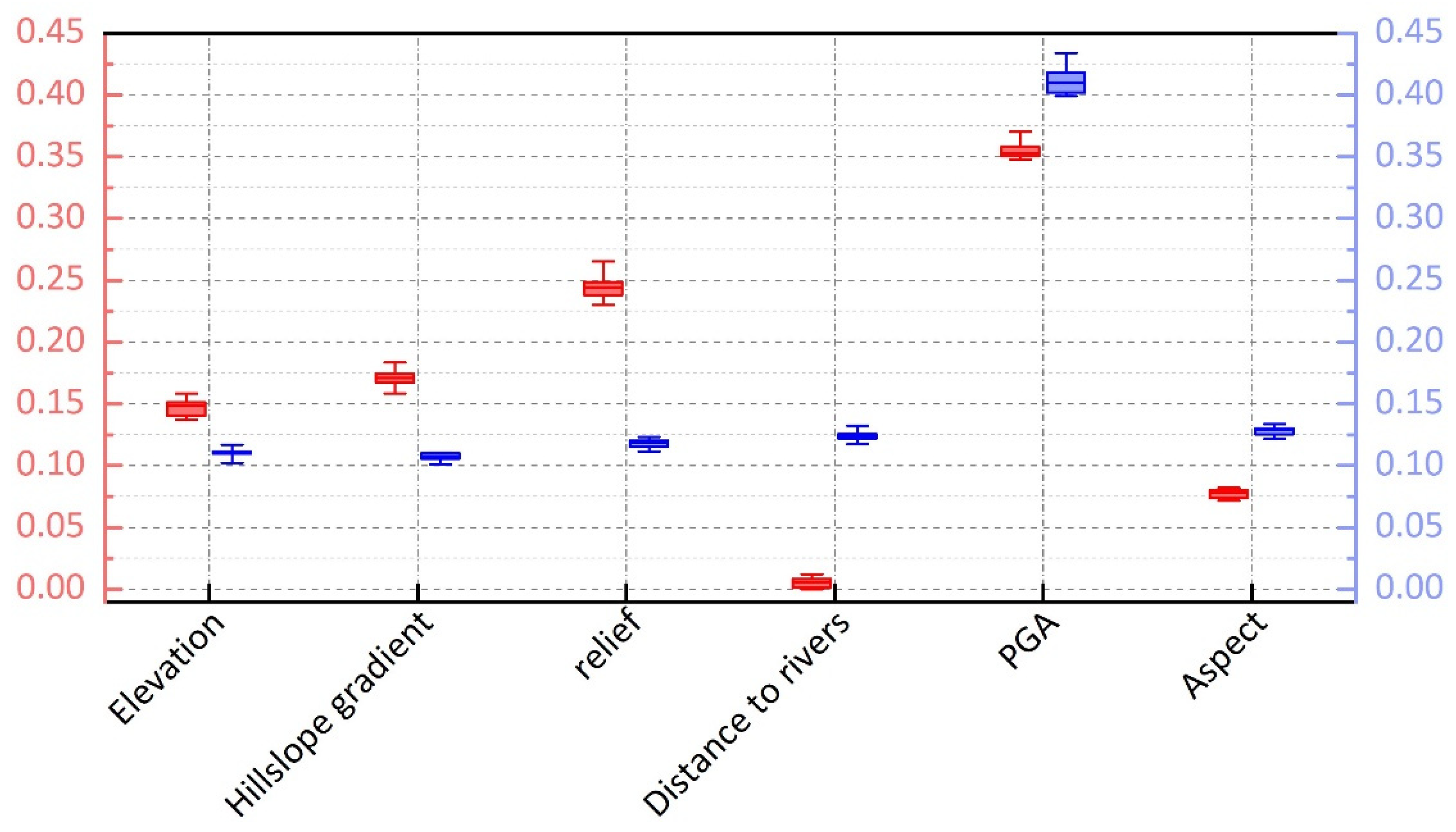
5.2. Relative Importance of the Influencing Factors

The susceptibility to landslides is influenced by a multitude of conditioning factors, which collectively contribute to its comprehensive effect [35,69]. Reichenbach et al. [35] analyzed the relevant studies about the LSM from 1983 to 2016, and the result shows that a total of 596 factors were examined in the susceptibility assessment, with an average of 9 influencing factors considered per model. Notably, the selection of these factors was predominantly based on subjective criteria relying on the experience of experts. Shao et al. [4] conducted a detailed analysis of the coseismic landslides of the Palu area, and the results showed that the landslide was most significantly affected by the seismic factors. Secondly, the landslide abundance index of this earthquake presents a clear correlation between and hillslope gradient, relief, and distance to the rivers. Therefore, we conducted a test to assess the relative importance of the seven continuous variables in the two models (Figure 14). The results revealed that seismic motion had the highest relative importance in both models, with a value of approximately 0.4. However, it should be noted that the relative importance of hillslope gradient and relief is slightly higher than other variables, while the RF model shows that, except for PGA, the relative importance of other influencing factors are roughly same, indicating that the control effect of these factors on the occurrence of landslides is essentially consistent. In general, our analyses indicate that the PGA plays the most significant role in the occurrence of landslides, which is consistent with the previous studies [4,51].

5.3. Comparisons of the RF Model with LR Model

Currently, various quantitative algorithms are employed for seismic LSM. However, each approach has its own set of advantages and limitations [34,35]. Therefore, we selected the two most widely used data-driven models for LSM. The results demonstrate that both models effectively predict the distribution of actual landslides. Furthermore, the densely populated areas of landslides are predominantly located in regions characterized by high LSI values. However, the AUC value of the RF model is slightly higher than that of the LR model, showing that the prediction ability of the RF model is better than the LR model [40,43]. This is mainly because the LR model encounters challenges related to quasi-complete separation issues when dealing with some categorical variable classes converted into dummy explanatory variables. In contrast, the RF model has demonstrated exceptional capability in effectively handling categorical predictors [34]. RF offers enhanced flexibility in evaluating intricate interactions among influencing factors for landslide susceptibility assessment. However, due to its linear features, LR is constrained by assumptions of normality and linearity, leading to limitations in addressing multiple or complex non-linear issues. As a result, LR tends to underperform in such scenarios. It should be noted that the RF model demonstrates superior predictive capabilities and operates as a non-parametric method. In contrast, the LR model offers the advantages of straightforward calculations and clear regression coefficients. Consequently, the LR model remains the most commonly employed model in LSM [34].

6. Conclusions

This paper aims at conducting the LSM associated with the 2018 Palu earthquake and estimating the quality of the most popular machine learning algorithms, the LR and RF models. The results were validated by the ROC curve and statistical measures. Based on the above work, the following main conclusions can be drawn:

(1)

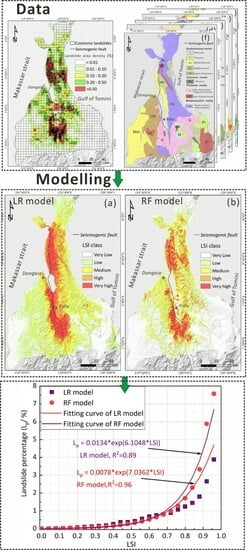
Based on the LSM predicted by two models and actual landslides, the landslide abundance area roughly matches the area of high LSI, with areas with LSI mainly concentrated along both sides of the seismogenic fault. The areas with high LSI mainly include the southern part of the epicenter and the areas on both sides of the Palu basin, which are also the landslide abundance areas.

(2)

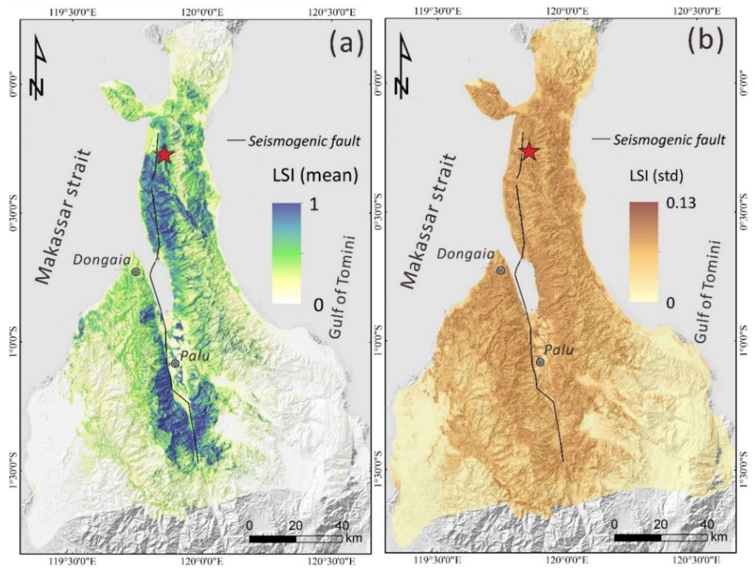
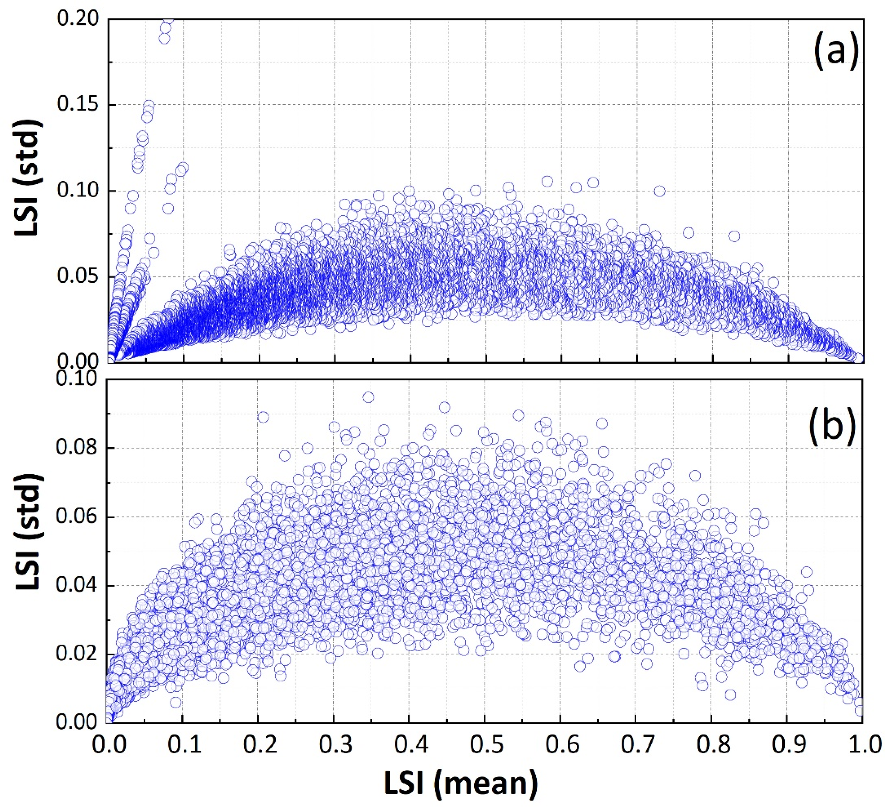
Compared to the LR model, the std of the RF model is smaller, with a max std of 0.13. The std based on the RF model is lower than that of the LR model, indicating that the evaluation results based on the RF model are less affected by the changes in training samples, while the predicted result of the LR model has a relatively large variation in LSI with the changes in training samples.

(3)

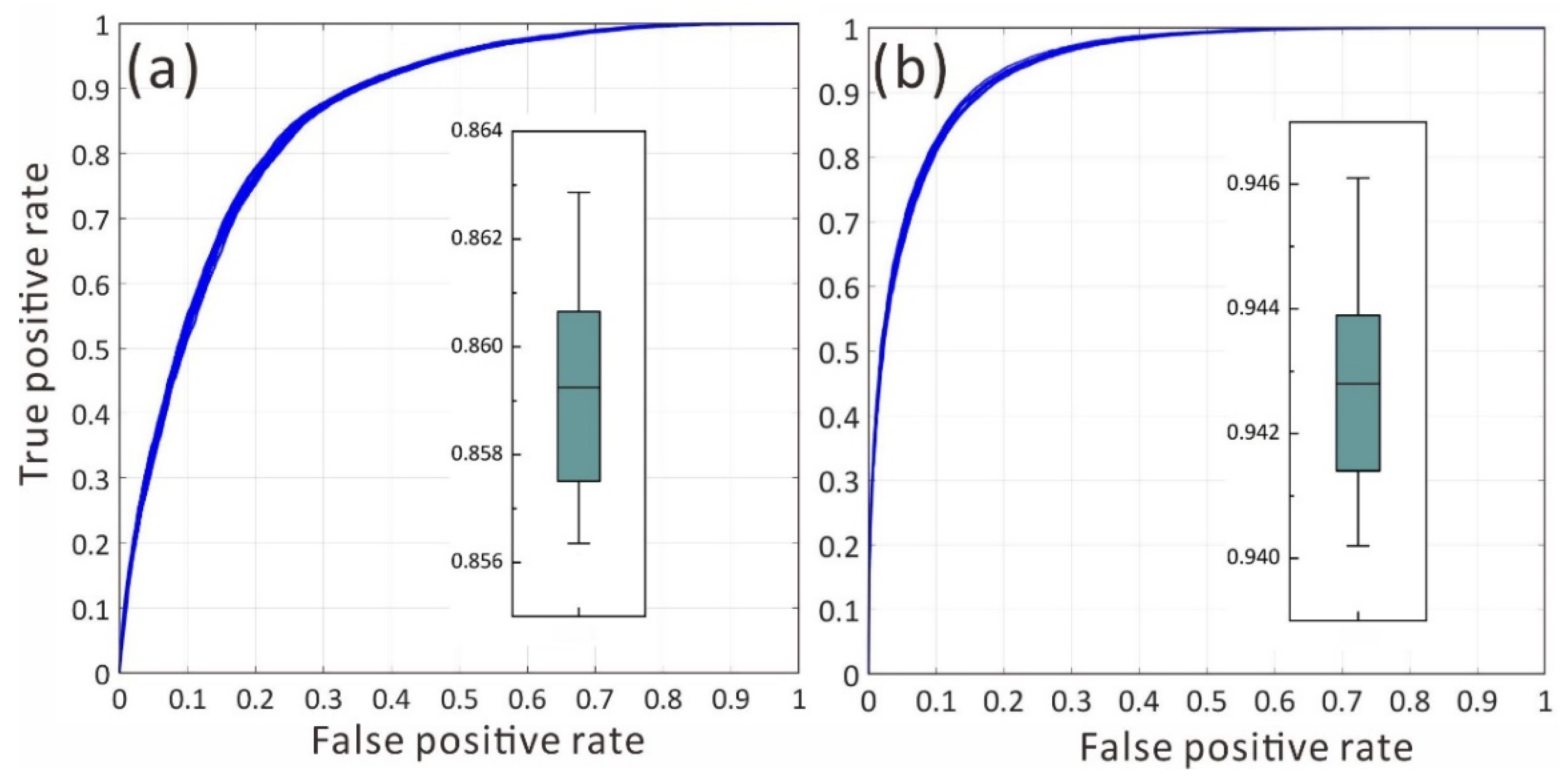
The assessment results based on the RF model are less affected by the changes in the training samples, while the predicted result of the LR model has a relatively large variation in LSI with the changes in the training samples. Both models demonstrate satisfactory performance; the RF model exhibits higher predictive capability compared to the LR model. The RF model, with a predicted rate of 0.94, is significantly higher than the rate of 0.86 for the LR model. Overall, the LR and RF models are useful tools for LSM of seismic events.

(4)

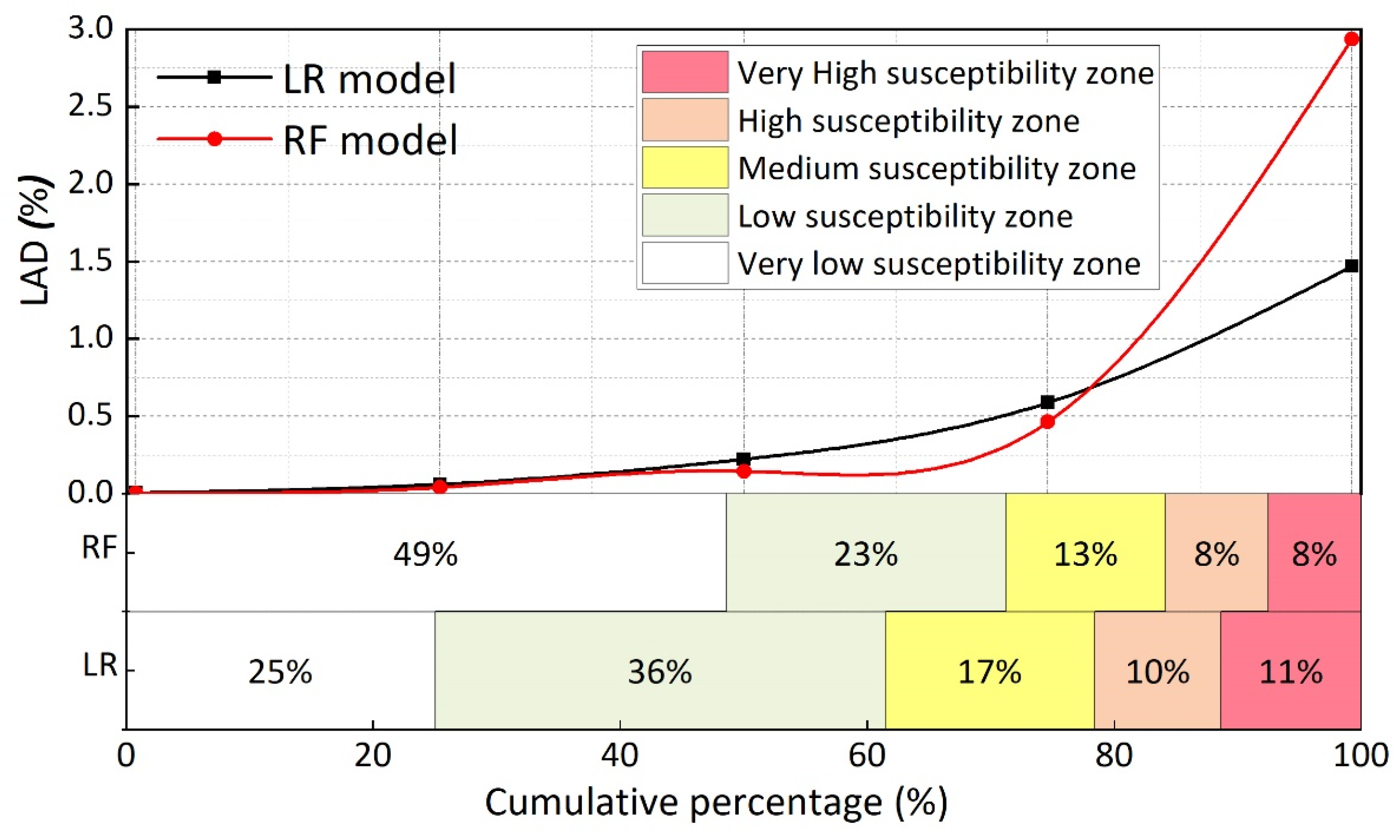
We calculate the probability of landslide occurrence and average LSI for each interval using 0.05 width bins, and then fit the relationship between LSI and landslide percentage (Lp). The results indicate that there is a clear exponential relationship between the LSI and the landslide percentage (Lp) of $L_p=0.0134\ast \mathrm{e}\mathrm{x}\mathrm{p}(6.1048\ast LSI)$ for the LR model and $L_p=0.0078\ast \mathrm{e}\mathrm{x}\mathrm{p}(7.0362\ast LSI)$ for the RF model. This equation can be used to correct the LSI to represent the landslide percentage (Lp) when the 1:1 ratio of landsliding/non-landsliding is used for modelling of the Palu area.

References

1. Fan, X.; Scaringi, G.; Korup, O.; West, A.J.; van Westen, C.J.; Tanyas, H.; Hovius, N.; Hales, T.C.; Jibson, R.W.; Allstadt, K.E.; et al. Earthquake-induced chains of geologic hazards: Patterns, mechanisms, and impacts. Rev. Geophys. 2019, 57, 421–503. [Google Scholar] [CrossRef]
2. Gorum, T.; van Westen, C.J.; Korup, O.; van der Meijde, M.; Fan, X.; van der Meer, F.D. Complex rupture mechanism and topography control symmetry of mass-wasting pattern, 2010 Haiti earthquake. Geomorphology 2013, 184, 127–138. [Google Scholar] [CrossRef]
3. Havenith, H.B.; Guerrier, K.; Schlögel, R.; Braun, A.; Ulysse, S.; Mreyen, A.S.; Victor, K.H.; Saint-Fleur, N.; Cauchie, L.; Boisson, D.; et al. Earthquake-induced landslides in Haiti: Analysis of seismotectonic and possible climatic influences. Nat. Hazards Earth Syst. Sci. 2022, 22, 3361–3384. [Google Scholar] [CrossRef]
4. Shao, X.; Ma, S.; Xu, C. Distribution and characteristics of shallow landslides triggered by the 2018 Mw 7.5 Palu earthquake, Indonesia. Landslides 2023, 20, 157–175. [Google Scholar] [CrossRef]
5. Shao, X.; Ma, S.; Xu, C.; Zhang, P.; Wen, B.; Tian, Y.; Zhou, Q.; Cui, Y. Planet Image-Based Inventorying and Machine Learning-Based Susceptibility Mapping for the Landslides Triggered by the 2018 Mw6.6 Tomakomai, Japan Earthquake. Remote Sens. 2019, 11, 978. [Google Scholar] [CrossRef]
6. Zhao, B.; Hu, K.; Yang, Z.; Liu, Q.; Zou, Q.; Chen, H.; Zhang, W.; Zhu, L.; Su, L.-J. Geomorphic and tectonic controls of landslides induced by the 2022 Luding earthquake. J. Mt. Sci. 2022, 19, 3323–3345. [Google Scholar] [CrossRef]
7. Shao, X.; Xu, C.; Ma, S. Preliminary analysis of coseismic landslides induced by the 1 June 2022 Ms 6.1 Lushan Earthquake, China. Sustainability 2022, 14, 16554. [Google Scholar] [CrossRef]
8. Gorum, T.; Korup, O.; van Westen, C.J.; van der Meijde, M.; Xu, C.; van der Meer, F.D. Why so few? Landslides triggered by the 2002 Denali earthquake, Alaska. Quat. Sci. Rev. 2014, 95, 80–94. [Google Scholar] [CrossRef]
9. Shao, X.; Xu, C.; Ma, S.; Shyu, J.; Zhou, Q. Calculation of landslide occurrence probability in Taiwan region under different ground motion conditions. J. Mt. Sci. 2021, 18, 1003–1012. [Google Scholar] [CrossRef]
10. Robinson, T.R.; Rosser, N.J.; Densmore, A.L.; Williams, J.G.; Kincey, M.E.; Benjamin, J.; Bell, H.J.A. Rapid post-earthquake modelling of coseismic landslide intensity and distribution for emergency response decision support. Nat. Hazards Earth Syst. Sci. 2017, 17, 1521–1540. [Google Scholar] [CrossRef]
11. Lombardo, L.; Bakka, H.; Tanyas, H.; Westen, C.; Mai, P.M.; Huser, R. Geostatistical Modeling to Capture Seismic-Shaking Patterns From Earthquake-Induced Landslides. J. Geophys. Res. Earth Surf. 2019, 124, 1958–1980. [Google Scholar] [CrossRef]
12. Chalkias, C.; Ferentinou, M.; Polykretis, C. GIS-Based Landslide Susceptibility Mapping on the Peloponnese Peninsula, Greece. Geosciences 2014, 4, 176–190. [Google Scholar] [CrossRef]
13. Parker, R.N.; Densmore, A.L.; Rosser, N.J.; de Michele, M.; Li, Y.; Huang, R.; Whadcoat, S.; Petley, D.N. Mass wasting triggered by the 2008 Wenchuan earthquake is greater than orogenic growth. Nat. Geosci. 2011, 4, 449–452. [Google Scholar] [CrossRef]
14. Xiong, J.; Chen, M.; Tang, C. Long-term changes in the landslide sediment supply capacity for debris flow occurrence in Wenchuan County, China. Catena 2021, 203, 105340. [Google Scholar] [CrossRef]
15. Tian, Y.; Owen, L.A.; Xu, C.; Ma, S.; Li, K.; Xu, X.; Figueiredo, P.M.; Kang, W.; Guo, P.; Wang, S.; et al. Landslide development within 3 years after the 2015 Mw 7.8 Gorkha earthquake, Nepal. Landslides 2020, 17, 1251–1267. [Google Scholar] [CrossRef]
16. Ma, S.; Xu, C.; Shao, X. Spatial prediction strategy for landslides triggered by large earthquakes oriented to emergency response, mid-term resettlement and later reconstruction. Int. J. Disaster Risk Reduct. 2020, 43, 101362. [Google Scholar] [CrossRef]
17. Massey, C.; Townsend, D.; Rathje, E.; Allstadt, K.E.; Lukovic, B.; Kaneko, Y.; Bradley, B.; Wartman, J.; Jibson, R.W.; Petley, D.N.; et al. Landslides Triggered by the 14 November 2016 Mw 7.8 Kaikōura Earthquake, New Zealand. Bull. Seismol. Soc. Am. 2018, 108, 1630–1648. [Google Scholar] [CrossRef]
18. Chen, Z.; Song, D. Modeling landslide susceptibility based on convolutional neural network coupling with metaheuristic optimization algorithms. Int. J. Digit. Earth 2023, 16, 3384–3416. [Google Scholar] [CrossRef]
19. Huang, F.; Yan, J.; Fan, X.; Yao, C.; Huang, J.; Chen, W.; Hong, H. Uncertainty pattern in landslide susceptibility prediction modelling: Effects of different landslide boundaries and spatial shape expressions. Geosci. Front. 2022, 13, 101317. [Google Scholar] [CrossRef]
20. Chen, X.L.; Liu, C.G.; Yu, L.; Lin, C.X. Critical acceleration as a criterion in seismic landslide susceptibility assessment. Geomorphology 2014, 217, 15–22. [Google Scholar] [CrossRef]
21. Huang, D.; Wang, G.; Du, C.; Jin, F.; Feng, K.; Chen, Z. An integrated SEM-Newmark model for physics-based regional coseismic landslide assessment. Soil Dyn. Earthq. Eng. 2020, 132, 106066. [Google Scholar] [CrossRef]
22. Newmark, N.M. Effects of earthquakes on dams and embankments. Géotechnique 1965, 15, 139–160. [Google Scholar] [CrossRef]
23. Wang, T.; Wu, S.R.; Shi, J.S.; Xin, P.; Wu, L.Z. Assessment of the effects of historical strong earthquakes on large-scale landslide groupings in the Wei River midstream. Eng. Geol. 2018, 235, 11–19. [Google Scholar] [CrossRef]
24. Jibson, R.W. Methods for assessing the stability of slopes during earthquakes—A retrospective. Eng. Geol. 2011, 122, 43–50. [Google Scholar] [CrossRef]
25. Jibson, R.W.; Harp, E.L.; Michael, J.A. A method for producing digital probabilistic seismic landslide hazard maps: An example from the Los Angeles, California, area. Eng. Geol. 2000, 58, 271–289. [Google Scholar] [CrossRef]
26. Godt, J.W.; Sener, B.; Verdin, K.L.; Wald, D.J.; Earle, P.S.; Harp, E.L.; Jibson, R.W. Rapid assessment of earthquake-induced landsliding. In Proceedings of the First World Landslide Forum, Tokyo, Japan, 18–21 November 2008. [Google Scholar]
27. Ma, S.Y.; Xu, C. Assessment of co-seismic landslide hazard using the Newmark model and statistical analyses: A case study of the 2013 Lushan, China, Mw6.6 earthquake. Nat. Hazards 2019, 96, 389–412. [Google Scholar] [CrossRef]
28. Chen, X.; Liu, C.; Wang, M. A method for quick assessment of earthquake-triggered landslide hazards: A case study of the Mw6.1 2014 Ludian, China earthquake. Bull. Eng. Geol. Environ. 2019, 78, 2449–2458. [Google Scholar] [CrossRef]
29. Gallen, S.F.; Clark, M.K.; Godt, J.W.; Roback, K.; Niemi, N.A. Application and evaluation of a rapid response earthquake-triggered landslide model to the 25 April 2015 Mw 7.8 Gorkha earthquake, Nepal. Tectonophysics 2017, 714–715, 173–187. [Google Scholar] [CrossRef]
30. Yue, X.; Wu, S.; Yin, Y.; Gao, J.; Zheng, J. Risk Identification of Seismic Landslides by Joint Newmark and RockFall Analyst Models: A Case Study of Roads Affected by the Jiuzhaigou Earthquake. Int. J. Disaster Risk Sci. 2018, 9, 392–406. [Google Scholar] [CrossRef]
31. Du, G.; Zhang, Y.; Zou, L.; Yang, Z.; Yuan, Y.; Ren, S. Co-seismic landslide hazard assessment of the 2017 Ms 6.9 Milin earthquake, Tibet, China, combining the logistic regression–information value and Newmark displacement models. Bull. Eng. Geol. Environ. 2022, 81, 446. [Google Scholar] [CrossRef]
32. Dreyfus, D.K.; Rathje, E.M.; Jibson, R.W. The influence of different simplified sliding-block models and input parameters on regional predictions of seismic landslides triggered by the Northridge earthquake. Eng. Geol. 2013, 163, 41–54. [Google Scholar] [CrossRef]
33. Guzzetti, F.; Carrara, A.; Cardinali, M.; Paola, R. Landslide hazard evaluation: A review of current techniques and their application in a multi-scale study, Central Italy. Geomorphology 1999, 31, 181–216. [Google Scholar] [CrossRef]
34. Merghadi, A.; Yunus, A.P.; Dou, J.; Whiteley, J.; ThaiPham, B.; Bui, D.T.; Avtar, R.; Abderrahmane, B. Machine learning methods for landslide susceptibility studies: A comparative overview of algorithm performance. Earth-Sci. Rev. 2020, 207, 103225. [Google Scholar] [CrossRef]
35. Reichenbach, P.; Rossi, M.; Malamud, B.D.; Mihir, M.; Guzzetti, F. A review of statistically-based landslide susceptibility models. Earth-Sci. Rev. 2018, 180, 60–91. [Google Scholar] [CrossRef]
36. Hong, H.; Pradhan, B.; Xu, C.; Tien Bui, D. Spatial prediction of landslide hazard at the Yihuang area (China) using two-class kernel logistic regression, alternating decision tree and support vector machines. Catena 2015, 133, 266–281. [Google Scholar] [CrossRef]
37. Kavzoglu, T.; Sahin, E.K.; Colkesen, I. An assessment of multivariate and bivariate approaches in landslide susceptibility mapping: A case study of Duzkoy district. Nat. Hazards 2015, 76, 471–496. [Google Scholar] [CrossRef]
38. Xu, C.; Xu, X.; Dai, F.; Saraf, A.K. Comparison of different models for susceptibility mapping of earthquake triggered landslides related with the 2008 Wenchuan earthquake in China. Comput. Geosci. 2012, 46, 317–329. [Google Scholar] [CrossRef]
39. Arabameri, A.; Chandra Pal, S.; Rezaie, F.; Chakrabortty, R.; Saha, A.; Blaschke, T.; Di Napoli, M.; Ghorbanzadeh, O.; Thi Ngo, P.T. Decision tree based ensemble machine learning approaches for landslide susceptibility mapping. Geocarto Int. 2021, 37, 4594–4627. [Google Scholar] [CrossRef]
40. He, Q.; Wang, M.; Liu, K. Rapidly assessing earthquake-induced landslide susceptibility on a global scale using random forest. Geomorphology 2021, 391, 107889. [Google Scholar] [CrossRef]
41. Sahin, E.K. Implementation of free and open-source semi-automatic feature engineering tool in landslide susceptibility mapping using the machine-learning algorithms RF, SVM, and XGBoost. Stoch. Environ. Res. Risk Assess. 2023, 37, 1067–1092. [Google Scholar] [CrossRef]
42. Wang, Y.; Fang, Z.; Hong, H. Comparison of convolutional neural networks for landslide susceptibility mapping in Yanshan County, China. Sci. Total Environ. 2019, 666, 975–993. [Google Scholar] [CrossRef] [PubMed]
43. Pourghasemi, H.R.; Rahmati, O. Prediction of the landslide susceptibility: Which algorithm, which precision? Catena 2018, 162, 177–192. [Google Scholar] [CrossRef]
44. Hall, R. Cenozoic geological and plate tectonic evolution of SE Asia and the SW Pacific: Computer-based reconstructions, model and animations. J. Asian Earth Sci. 2002, 20, 353–431. [Google Scholar] [CrossRef]
45. Puntodewo, S.S.O.; McCaffrey, R.; Calais, E.; Bock, Y.; Rais, J.; Subarya, C.; Poewariardi, R.; Stevens, C.; Genrich, J.; Fauzi; et al. GPS measurements of crustal deformation within the Pacific-Australia plate boundary zone in Irian Jaya, Indonesia. Tectonophysics 1994, 237, 141–153. [Google Scholar] [CrossRef]
46. Wallace, L.M.; McCaffrey, R.; Beavan, J.; Ellis, S. Rapid microplate rotations and backarc rifting at the transition between collision and subduction. Geology 2005, 33, 857–860. [Google Scholar] [CrossRef]
47. Socquet, A.; Hollingsworth, J.; Pathier, E.; Bouchon, M. Evidence of supershear during the 2018 magnitude 7.5 Palu earthquake from space geodesy. Nat. Geosci. 2019, 12, 192–199. [Google Scholar] [CrossRef]
48. Watkinson, I.; Hall, R. Fault systems of the eastern Indonesian triple junction: Evaluation of Quaternary activity and implications for seismic hazards. Geol. Soc. Lond. Spec. Publ. 2017, 441, 71–120. [Google Scholar] [CrossRef]
49. Watkinson, I. Ductile flow in the metamorphic rocks of central Sulawesi. Geol. Soc. Lond. Spec. Publ. 2011, 355, 157–176. [Google Scholar] [CrossRef]
50. Natawidjaja, D.H.; Daryono, M.R.; Prasetya, G.; Liu, P.L.; Hananto, N.D.; Kongko, W.; Triyoso, W.; Puji, A.R.; Meilano, I.; Gunawan, E.; et al. The 2018 Mw7.5 Palu ‘supershear’ earthquake ruptures geological fault’s multisegment separated by large bends: Results from integrating field measurements, LiDAR, swath bathymetry and seismic-reflection data. Geophys. J. Int. 2020, 224, 985–1002. [Google Scholar] [CrossRef]
51. Zhao, B. Landslides triggered by the 2018 Mw 7.5 Palu supershear earthquake in Indonesia. Eng. Geol. 2021, 294, 106406. [Google Scholar] [CrossRef]
52. Nowicki Jessee, M.A.; Hamburger, M.W.; Allstadt, K.; Wald, D.J.; Robeson, S.M.; Tanyas, H.; Hearne, M.; Thompson, E.M. A global empirical model for near-real-time assessment of seismically induced landslides. J. Geophys. Res. Earth Surf. 2019, 123, 1835–1859. [Google Scholar] [CrossRef]
53. Indonesian Geospatial Information Agency. DEMNAS—Seamless Digital Elevation Model (DEM) Dan Batimetri Nasional. 2019. Available online: http://tides.big.go.id/DEMNAS/ (accessed on 18 January 2019).
54. van Leeuwen, T.M. Stratigraphy and tectonic setting of the Cretaceous and Paleogene volcanic-sedimentary successions in northwest Sulawesi, Indonesia: Implications for the Cenozoic evolution of Western and Northern Sulawesi. J. Asian Earth Sci. 2005, 25, 481–511. [Google Scholar] [CrossRef]
55. USGS. United States Geological Survey. 2018. Available online: https://earthquake.usgs.gov/earthquakes/eventpage/us1000h3p4/executive (accessed on 18 January 2019).
56. Dai, F.C.; Lee, C.F. Landslide characteristics and slope instability modeling using GIS, Lantau Island, Hong Kong. Geomorphology 2002, 42, 213–228. [Google Scholar] [CrossRef]
57. Budimir, M.E.A.; Atkinson, P.M.; Lewis, H.G. A systematic review of landslide probability mapping using logistic regression. Landslides 2015, 12, 419–436. [Google Scholar] [CrossRef]
58. Tanyas, H.; Rossi, M.; Alvioli, M.; van Westen, C.J.; Marchesini, I. A global slope unit-based method for the near real-time prediction of earthquake-induced landslides. Geomorphology 2019, 327, 126–146. [Google Scholar] [CrossRef]
59. Shao, X.; Ma, S.; Xu, C.; Zhou, Q. Effects of sampling intensity and non-slide/slide sample ratio on the occurrence probability of coseismic landslides. Geomorphology 2020, 363, 107222. [Google Scholar] [CrossRef]
60. Breiman, L. Random Forests. Mach. Learn. 2001, 45, 5–32. [Google Scholar] [CrossRef]
61. Genuer, R.; Poggi, J.-M.; Tuleau-Malot, C. Variable selection using random forests. Pattern Recognit. Lett. 2010, 31, 2225–2236. [Google Scholar] [CrossRef]
62. Bureau, A.; Dupuis, J.; Hayward, B.; Falls, K.; Van Eerdewegh, P. Mapping complex traits using Random Forests. BMC Genet. 2003, 4, S64. [Google Scholar] [CrossRef]
63. Stumpf, A.; Kerle, N. Object-oriented mapping of landslides using Random Forests. Remote Sens. Environ. 2011, 115, 2564–2577. [Google Scholar] [CrossRef]
64. Tien Bui, D.; Tuan, T.A.; Klempe, H.; Pradhan, B.; Revhaug, I. Spatial prediction models for shallow landslide hazards: A comparative assessment of the efficacy of support vector machines, artificial neural networks, kernel logistic regression, and logistic model tree. Landslides 2016, 13, 361–378. [Google Scholar] [CrossRef]
65. Cantarino, I.; Carrion, M.A.; Goerlich, F.; Martinez Ibañez, V. A ROC analysis-based classification method for landslide susceptibility maps. Landslides 2018, 16, 265–282. [Google Scholar] [CrossRef]
66. Brenning, A. Spatial prediction models for landslide hazards: Review, comparison and evaluation. Nat. Hazards Earth Syst. Sci. 2005, 5, 853–862. [Google Scholar] [CrossRef]
67. Hong, H.; Miao, Y.; Liu, J.; Zhu, A.X. Exploring the effects of the design and quantity of absence data on the performance of random forest-based landslide susceptibility mapping. Catena 2019, 176, 45–64. [Google Scholar] [CrossRef]
68. Lee, C.T. Statistical seismic landslide hazard analysis: An example from Taiwan. Eng. Geol. 2014, 182, 201–212. [Google Scholar] [CrossRef]
69. Shao, X.; Xu, C. Earthquake-induced landslides susceptibility assessment: A review of the state-of-the-art. Nat. Hazards Res. 2022, 2, 172–182. [Google Scholar] [CrossRef]
Figure 1. Mapping showing the distribution of aftershocks, topography, and structural features of the 2018 Mw 7.5 Palu earthquake.
Remotesensing 15 04733 g001
Figure 2. Map showing the spatial distribution of the coseismic landslides of the Palu earthquake.
Remotesensing 15 04733 g002
Figure 3. Map showing the influencing factors used for the landslide susceptibility modelling; (a) Hillslope gradient and drainages distribution; (b) Topographic relief; (c) Aspect; (d) Peak ground acceleration (PGA); (e) Peak ground velocity (PGV); (f) Lithology.
Remotesensing 15 04733 g003aRemotesensing 15 04733 g003b
Figure 4. The correlation coefficient matrix of the factors used for modelling.
Remotesensing 15 04733 g004
Figure 5. Map showing the mean landslide susceptibility index (LSI) and model uncertainty for the LR model; (a) the result of mean LSI yielding 20 predicted pictures; (b) The result of standard deviation (std) for model uncertainty. The red polygons represent the coseismic landslides.
Remotesensing 15 04733 g005
Figure 6. Map showing the mean landslide susceptibility index (LSI) and model uncertainty for the RF model; (a) the result of mean LSI yielding 20 predicted pictures; (b) The result of standard deviation (std) for model uncertainty.
Remotesensing 15 04733 g006
Figure 7. Scatter plot showing the relationship between the average LSI and standard deviation (std) of the two different models. (a) LR model; (b) RF model. The circles represent the grid cells.
Remotesensing 15 04733 g007
Figure 8. Map showing the frequency density distribution of LSI for two different models; (a) LR model; (b) RF model.
Remotesensing 15 04733 g008
Figure 9. Landslide susceptibility class map of two different model; (a) LR model; (b) RF model.
Remotesensing 15 04733 g009
Figure 10. The statistical results of the predicted area and the landslide number density (LND) distribution under LSI class for two models.
Remotesensing 15 04733 g010
Figure 11. Prediction curves of 20 maps of landslide susceptibility mapping using two models. (a) LR model; (b) RF model.
Remotesensing 15 04733 g011
Figure 12. Map showing the relationship of LSI between LR-based and RF-based landslide susceptibility assessment results.
Remotesensing 15 04733 g012
Figure 13. Relationship between LSI and landslide percentage used to represent the actual occurrence probability of the landslide.
Remotesensing 15 04733 g013
Figure 14. Map showing the relative importance of the continuous variables for two models; the red and blue boxes represent the LR and RF models, respectively.
Remotesensing 15 04733 g014
Disclaimer/Publisher’s Note: The statements, opinions and data contained in all publications are solely those of the individual author(s) and contributor(s) and not of MDPI and/or the editor(s). MDPI and/or the editor(s) disclaim responsibility for any injury to people or property resulting from any ideas, methods, instructions or products referred to in the content.