Applicability Assessment of GPM IMERG Satellite Heavy-Rainfall-Informed Reservoir Short-Term Inflow Forecast and Optimal Operation: A Case Study of Wan’an Reservoir in China

Abstract

Satellite precipitation estimate (SPE) dedicated to reservoir inflow forecasting is very attractive as it can provide near-real-time information for reservoir monitoring. However, the potential of SPE retrievals with fine temporal resolution in supporting the high-quality pluvial flood inflow forecast and robust short-term operation of a reservoir remains unclear. In this study, the hydrological applicability of half-hourly Integrated Multisatellite Retrievals for Global Precipitation Measurement (GPM IMERG) heavy rainfall data was explored using a synthetic experiment of flood inflow forecast at sub-daily to daily lead times and resultant reservoir short-term operation. The event-based flood forecast was implemented via the rainfall–runoff model GR4H driven by the forecasted IMERG. Then, inflow forecast-informed reservoir multi-objective optimal operation was conducted via a numerical reservoir system and assessed by the risk-based robustness indices encompassing reliability, resilience, vulnerability for water supply, and flood risk ratio for flood prevention. Selecting the Wan’an reservoir located in eastern China as the test case, the results show that the flood forecast forced with IMERG exhibits slightly lower accuracy than that driven by the gauge rainfall across varying lead times. For a specific robustness index, its trends between IMERG and gauge rainfall inputs are comparable, while its magnitude depends on varying lead times and scale ratios (i.e., the reservoir scale). The pattern that the forecast errors in IMERG increase with the lead time is changed in the resultant inflow forecast series and dynamics in the robustness indices for the optimal operation decision. This indicates that the flood forecast model coupled with reservoir operation system could partly compensate the original SPE errors. Our study highlights the acceptable hydrological applicability of IMERG rainfall towards reservoir inflow forecast for robust operation, despite the intrinsic error in SPE.

1. Introduction

Numerous investigations were carried out on the direct hydrological application of typical satellite precipitation estimate (SPE) retrievals and manifest that the hydrological modeling accuracy depends on various factors. It was concluded that the performance of SPE-driven hydrological models was strongly influenced by precipitation type, seasonality, hydrological model formulation, and topography [1,2]. The applicability of several SPEs (CMORPH, 3B42RT, 3B42, and PERSIANN) forcing a hydrologic model to simulate daily streamflow in two highland watersheds was evaluated, and a similar result was also found that the modeling performance largely depends on the SPE type, with 3B42RT and CMORPH showing modest skills and underestimation of high flood peaks, and 3B42 and PERSIANN showing poor skills [3]. Previous studies further suggested that the SPE suitability in hydrological simulation relies on the product versions, even for the same measurement mission [4]. Specifically, taking the Integrated Multisatellite Retrievals for Global Precipitation Measurement (IMERG) product as an example, the post-processed “final” version, usually used for research, is generally superior to the near-real-time “late” and “early” versions [5], and both V04 and V05 of the “final” run outperform V03 significantly [6]. Although the “early” and V03 IMERG have relatively lower performance in precipitation, they were proved to be able to provide acceptable application efficiency in many hydrological modeling cases [7,8,9] and to achieve higher reliability after bias correction [10,11]. In addition to these individual factors, multiple factors might interactively impact the hydrological modeling performance. In a recent study, the applicability of six fine-resolution SPE products (including 3B42, 3B42RT, and PERSIANN, among others) to hydrologic modeling in a small basin in China was assessed, and this study revealed that although the SPE-based products are not as accurate as the gauge-based data, they could obtain better performance in discharge simulations when combined with an appropriate hydrological model [12]. In addition, both the SPE measuring and SPE-forced hydrological modeling accuracy are shown to rely on the temporal resolution on which the evaluation is based [2]. For instance, in a study of the capability of 3B42RT, CMORPH, and PERSIANN to estimate large rainfall rates at various temporal accumulations across the US, it was suggested that none of the fine temporal resolution (3 hourly) products were ideal for monitoring heavy precipitation. Furthermore, as accumulation time gets longer, the probability of detection improves and the false alarm ratio decreases, which might largely impact the hydrologic modeling efficiency [13]. Another attempt was presented, which carried out a comprehensive evaluation of two GPM-IMERG products, specifically IMERG-Final-Run (FR) and IMERG-Real-Time (RT) [14]. For entire spectrum precipitation rates (p ≥ 0.1 mm), 1, 3, 6-hourly IMERG-FR did not show a clear improvement of the bias over IMERG-RT, while for 12-hourly and daily precipitation estimates, the bias in IMERG-FR has improved compared to IMERG-RT.

Another hydrological application of SPE is to forecast rainfall and indirectly support the hydrological forecast. Studies proved that merging SPE products also has benefits for improving the rainfall forecast across varying regions and basins. For example, IMERG data were used to increase the rainfall forecast in high spatiotemporal resolution in Indonesia areas [15] and Niger River basin [16].

Reservoir operation plays a critical role in making efficient water planning. To operate reservoirs, policies are developed to determine the volume of water to be stored and/or discharged at a given time according to the state of the reservoir inflow, magnitude of demands, vacant storage capacity, and hydrological conditions in areas downstream to the reservoir [17]. Among various factors influencing the operation system, inflow, especially in pluvial flood events, imposes a profound effect on operation decision. For example, the efficacy of flood control operation is largely related to the accuracy of inflow forecast [18].The advent of the satellite measurement mission provides a unique opportunity to overcome the traditional limitations of reservoir hydro-meteorological regime monitoring. Specifically, due to the features of near-real-time retrieval and fine temporal resolution, SPE is beneficial for short-term forecasting and nowcasting of reservoir inflow. Consequently, the use of SPE products in inflow modeling and forecasting has opened new venues to support reservoir water management. However, hours-long spaceborne heavy rainfall data are scarcely used in the reservoir inflow process, despite the abundance of SPE-forced rainfall–runoff modeling. On the other hand, the current reservoir inflow forecast primarily focuses on improving the forecast model, such as data-driven statistical analysis approaches and deep learning approaches [19,20], and physical-process-based hydrological models [21,22]. By contrast, the rainfall input data, which is traditionally provided by rain gauge stations, are rarely analyzed to quantify its impact on inflow forecast and resultant operation results. In summary, the SPE applicability in inflow forecast and resulting operation has been poorly understood so far, although SPE could provide near-real-time precipitation with fine resolution in hydraulic engineering management.

In the present study, to explore the applicability of IMERG heavy rainfall in supporting reservoir inflow forecast and resultant optimal operation, we conducted a series of hypothetical forecast and operation experiments in a reservoir system. First, a machine learning approach was used to generate synthetic forecasted heavy rainfall data. Then, the forecasted IMERG data that were used to forecast reservoir inflow and support operation were evaluated in terms of IMERG heavy rainfall detection accuracy, inflow forecasting accuracy, and optimal operation robustness. The objectives of the present study include: (1) whether the reservoir operation system behaviors robustly, when using inflow series forecasted via IMERG data; and (2) from sub-daily to daily scales, what impact does the varying lead times of inflow forecasted via IMERG data have on the inflow forecast accuracy and operation robustness?

This paper is organized into five sections. Section 2 provides the information about the study area and reservoir, and the data used. The methodologies, including the storm data generator, the rainfall–runoff model Génie Rural à 4 paramètres Horaires (GR4H), the reservoir system, and robustness assessment indices are introduced in Section 3. Section 4 presents the results of SPE accuracy, the inflow forecasting performance with SPE, and the robustness analysis on water supply and flood control of reservoir operation with SPE-forced inflow forecast. Discussion, limitation, and future works are presented in Section 5. Section 6 summarizes the conclusions and major findings.

2. Study Area and Materials

2.1. Study Area and Reservoir

The proposed framework for testing the applicability of IMERG heavy rainfall data towards inflow forecast and reservoir operation was applied to the Wan’an reservoir and its discharging area, i.e., the Wan’an basin (Figure 1). The dam site of the Wan’an reservoir is located at the upper reach of midstream Gan River in China, with an average annual discharge of 29.7 billion m³. The Wan’an reservoir controls a discharging area of 36,900 km², which accounts for 44.2% of the Gan River basin’s total area and lies within the humid climate zone of the mid-subtropical monsoon climate area. The mean annual temperature is 18.5 °C, and the annual precipitation is approximately 1560 mm (68.7% from April to September).

As the Gan River’s largest reservoir, the Wan’an reservoir was built in 1990, aiming to increase comprehensive benefits of flood prevention, power generation, irrigation, and aquaculture, among others. The Wan’an reservoir has a maximum capacity of 2106 Mm³ with a probable maximum flood water level of 103 m. The operation rules of the Wan’an reservoir include (1) to guarantee hydro-junction safety and enhance downstream flood prevention, and (2) to release water with a maximum flow of 36,700 m³/s at 103 m water level. This regulating capability results in smoothing inflow variation.

2.2. Hydro-Meteorological Data

IMERG is the level 3 multi-satellite precipitation algorithm of Integrated Multisatellite Retrievals for Global Precipitation Measurement (GPM), with the intention of creating a new generation of quasi-global precipitation products [23,24]. As the successor of TMPA mission, the IMERG system combines all available constellation satellite microwave precipitation estimates, microwave-calibrated infrared (IR) estimates, and monthly ground gauge analyses [25]. IMERG provides three versions of the products, including the “early” run approximately 4 h after the observation time for providing a preliminary estimate, the “late” run approximately 12 h after the observation time as more date arrive, and the “final” run approximately 2 months after the observation month as research. For these three IMERG versions, in addition to the difference in sensor data latency, the “early” and late” estimates are produced in near real time and adjusted by climatological coefficients varying by month and location. In contrast, the “final” run product is produced in post real time after gauge adjustments to be consistent with the Global Precipitation Climatology Centre (GPCC) precipitation data. Therefore, the “final” run product is characterized by higher accuracy, particularly over land, while the “early” and “late” run products have higher timeliness which is appealing to storm monitoring and flood forecast. There are two types of precipitation field variables embedded in each IMERG version, i.e., precipitationCal and precipitationUncal. The former means a multisatellite precipitation estimate merged with gauge calibration, while the latter provides the original multi-satellite precipitation estimate. For more detailed description, readers can refer to the previous study [26]. In this study, the “early” run products of IMERG V06 (hereafter referred to as IMERG), which has the highest timeliness and thus is potentially beneficial for reservoir storm regime monitoring, are used. The heavy rainfall extracted from IMERG is statistically evaluated based on the ground gauge observation, and then forces a rainfall–runoff model to generate the forecasted reservoir inflow at multiple lead times. The raw spatial and temporal resolutions of the IMERG products are 0.1° × 0.1° and half hour, respectively. The 6 h heavy rainfall and flood inflow datasets used in this study were accumulated by half-hourly data.

As part of a reference monitoring network, 6 h heavy rainfall data were measured directly across the Wan’an basin and collected by 45 rain gauge stations for 31 storm events during 2014 to 2019. In addition, to generate synthetic forecasted heavy rainfall data, the ERA5 weather reanalysis dataset, including convective available potential energy, dew-point temperature, instantaneous 10 m wind gust, wind speed, U and V wind components at 10 m, temperature at 2 m, total cloud cover, and relative humidity were used as predictors.

Event-based 6 h flood data of the Wan’an basin’s outlet were obtained for 31 flood events also during the year of 2014 to 2019.

3. Methodology

A series of synthetic experiments, including storm stochastic generation based on ERA5 weather reanalysis and random forest algorithm, flood simulation using the rainfall–runoff model forced with forecasted rainfall, and reservoir optimal operation driven by forecasted flood inflow, were designed to evaluate the applicability of IMERG heavy rainfall regarding reservoir inflow forecast accuracy and optimal operation robustness (Figure 2). The R and ArcGIS platforms were used to process and visualize the IMERG data, respectively, and the hydrological model and reservoir operation model were applied to rainfall–runoff modeling and optimal operation, respectively.

3.1. Storm Stochastic Generator

To synthetically forecast the storm at varying lead times from sub-daily to daily scales, a storm stochastic generator was established using the random forest approach based on ERA5 weather reanalysis (see Section 2.2 for the details) and SPE (or rain gauge) heavy rainfall data during 31 storm events. The random process from historical meteorological information to heavy rainfall forecast depends on the random forest algorithm, which is a commonly used ensemble machine learning algorithm and aggregates results from multiple decision trees to reach a single result [26]. In this study, the random forest algorithm was introduced in handling both classification and regression problems of rainfall, as its ease of use and flexibility has fueled its adoption.

3.2. Flood Forecasting Based on GR4H Model

In this study, to identify the inflow forecast characterization with IMERG input at different lead times, the conceptual lumped rainfall–runoff model GR4H was established, so that the flood modeling performance, derived from the IMERG and gauge rainfall forecast scenarios, are compared with each other. The GR4H model [27] runs at an hourly time step and was developed based on the GR4J model formulation [28]. It was chosen for its ease of calibration and the good performance of the GR series prototypes across a wide range of river-flow regimes [29,30,31]. The function that controls water balance in the GR4H model consists of four parameters to be calibrated: the capacity of a soil moisture accounting store (X1) and of the routing store (X3), the time base of a unit hydrograph (X4), and one parameter representing the groundwater exchange coefficient (X2). X2 can be either positive or negative, indicating that the water exchange function can simulate both imports and exports of water with the underground (including connections with deep aquifers or surrounding basins). X3 can also be used to parameterize the outflow from the routing store. The routing part of the structure consists of two flow components routed by two unit hydrographs and a non-linear store. The latter is mainly responsible for low-flow simulations, along with percolation and/or leakage from the soil moisture accounting store. The groundwater exchange term is added to these two flow components of the routing module.

The IMERG data during heavy rainfall events over the Wan’an basin were extracted using the Wan’an basin boundary provided by DEM map. Because the lumped hydrological model was used, the gridded IMERG of the Wan’an basin was averaged over the basin area and then input into the model.

3.3. Reservoir System Construction

3.3.1. Reservoir Optimal Operation Model

Given the inflow input with forecast uncertainty for an upcoming time period, the reservoir optimal operation (e.g., controlled release flow, storage, and water level) can be identified by combining water balance (Equation (1)), operational constraints, and optimization algorithm. To achieve this, first, a multi-objective optimal operation model considering flood control, water supply, and amenity functions combined with the optimization algorithm of stochastic dynamic programming (SDP) was exploited. Second, each of the inflow series forecasted by the GR4H hydrological model at 6 h, 12 h, 24 h, 48 h, and 72 h lead times and the actual inflow series were used to drive the reservoir short-term operation model established in the first step. Third, different optimal operation series of using various forecast inflow inputs were compared with the optimal operation values of using the actual inflow:

$$S_{t-1}=S_t+Q_t-R_t, s.t. 0\le S\le S_{\max }$$

(1)

where S_t, Q_t, and R_t represent the storage water volume held in the reservoir, the inflow, and the controlled release at time step t, respectively; S_max denotes the reservoir capacity; evaporation can be ignored or accommodated by subtracting from the inflow time series so that Q_t refers to the net inflow. The demand of water can be represented by the target release constant or dynamic series. Therefore, this approach allows the analysis to capture the varying roles played by evaporation in different climate areas and water demand in different demand conditions.

The implementable procedure of SDP for determining an optimal operation decision was executed and simulated on all of these reservoir combinations using the R package reservoir [32]. The SDP function was used for water release policy design, which optimizes the release decisions via minimizing the sum of penalty costs incurred in the operation of the reservoir. The penalty costs are represented as a function of the volume of available water relative to the demand, as defined by Equation (2):

$$C_t={\left[1-(R_t/D)\right]}^{\tau }$$

(2)

where D is the water demand or target release, and $\tau$ is the penalty cost exponent on release, spill, and water level deviations from the target, which, when greater than one, drives the reservoir hedging the curtailment of release in order to avoid any reservoir failure that would result in larger damaging supply shortfalls. The $\tau$ was set to {2, 1, 4} in this study.

SDP can not only alleviate the deficiency of the dimensionality curse caused by dynamic programming, but also can use the hydrological state variable to capture forecasted hydrological conditions in its recursive equation and thus derive enhanced operating policies. The general form of the SDP’s backwards recursive procedure can be written as

$$f_t(S_t,Q_t)=\min \left\{C_t(S_t,Q_t,R_t)+E[f_{t+1}(S_{t+1},Q_{t+1})]\right\}, \forall S_t,Q_t and t\in \left\{1,\mathrm{\dots },T\right\}$$

(3)

where T is the number of operation time steps during a pluvial flood event. The reservoir state at each decision-making time step t is depicted by the storage S_t and the current period inflow Q_t. For each stage and time step, the release decision R_t is selected to minimize the current period cost $C_t(S_t,Q_t,R_t)$ plus future cost expectation $E[f_{t+1}(S_{t+1},Q_{t+1})]$, which depends on the resultant state of the system at next time step t + 1.

To simplify the operating schemes, the constant demand for water, i.e., target release constant, is assigned to all the alternative reservoirs by fixing the draft ratio (ratio of demand to mean inflow) at 0.2. Thirteen reservoir optimal operation scenarios were designed, which consist of the input scenarios for inflow forecasted using IMERG and gauge heavy rainfall at lead times of 0 h (the raw rainfall), 6 h, 12 h, 24 h, 48 h, and 72 h cases and the actual inflow.

3.3.2. Robustness Criteria of Reservoir Operation Assessment

The robustness is the ability of a system to generate close estimations under two different scenarios. In the present study, we have provided four risk-based statistical indices to evaluate the robustness of reservoir operation decision in short-time operation practices, which includes the reliability, resilience, and vulnerability (rrv) for water supply operation, and flood risk rate of exceeding a typical water level in flood control operation. Specifically, the rrv function of reservoir computes volumetric reliability, resilience, and dimensionless vulnerability based on simulations of reservoirs with specified capacity and target release that can be constant or time varying.

In the context of reservoir management, the reliability index is defined as the probability that a reservoir system would operate in a pre-defined environment without failure. Specifically, the concept of reliability is associated with reservoir storage–yield–performance techniques. For volumetric or quantity-based reliability, Re_v is defined as

$$R{e}_{\mathrm{v}}=V_s/V_{\mathrm{d}},0<R{e}_{\mathrm{v}}\le 1$$

(4)

where V_s and V_d denote the volume of water supplied and demand during the entire operation period, respectively. The duration of the ith failure event is denoted by d_i, and v_j represents the corresponding deficit which can be expressed as

$$v_j=1-{\displaystyle \sum _{t=1}^{d_i}(D_t-R_t)}$$

(5)

D_t and R_t are the target demand and the volume actually supplied during the tth period, respectively. It is worth noting that Re_v = 1 if D_t is totally satisfied, i.e., D_t = R_t for all t.

The resilience index ($\rho$) quantifies how quickly a reservoir is likely to recover from failure. The measure of $\rho$ adopted in this study follows the widely used definition:

$$\rho =\frac{f_s}{f_{\mathrm{d}}}, f_{\mathrm{d}}\ne 0$$

(6)

where f_s is the number of individual continuous sequences of failure periods and f_d is the total duration of all the failures; in other words, $\rho$ is the inverse of the average failure duration.

The vulnerability index measures the average volumetric severity of failure during a failure period and is mathematically expressed as

$${\eta }^{\text{'}}=\frac{{\displaystyle \sum _{j=1}^{f_s}\max (s_j)}}{f_{\mathrm{s}}}$$

(7)

where η′ is the vulnerability, S_j is the volumetric shortfall during jth continuous failure sequence, and f_s is the number of continuous failure sequences. As Equation (7) averages out the maximum shortfall over all the continuous failure periods, a reduction of f_s will cause η′ to increase when the numerator in Equation (7) remains unchanged. A practical situation where this may occur is when the reservoir capacity increases with all other factors remaining constant. One way to avoid this anomaly is to change the averaging in Equation (7). It is worth noting that η′ is in volumetric units; thus, a more useful formula of vulnerability is in dimensionless form defined by:

$$\eta =\frac{{\eta }^{\text{'}}}{D_{\mathrm{f}}}, 0 < \eta \le 1$$

(8)

where η is the dimensionless vulnerability metric, known as the vulnerability ratio in this study, and D_f is the (constant) target demand during failure.

Flood risk rate γ is defined as the ratio of the number of time steps occurring risk events to the total time steps in operation periods. The risk events combine three types of events in which the actual water level is higher than a typical water level (each of 95 m, 96 m, 97 m, 98 m, 99 m, and 100 m), the actual storage higher than a certain storage, or the actual maximum release greater than a certain flow corresponding to the concurrent water levels.

To identify the dynamism of robustness indices, as mentioned above, with varying reservoir states, the maximum depth of the reservoir descends from 103 m to 96 m with a 1 m interval, and the corresponding capacity, maximum surface area, and release vary according to the reservoir water level–capacity–area curve. The impact factor of these eight states in the reservoir denotes as scale ratio of the reservoir.

4. Results

The IMERG satellite grids are selected for statistical computation, heavy rainfall forecast, and flood forecast only if they cover at least one gauge station. Thirteen series of twelve pluvial flood inflow series generated using IMERG and gauge rainfall and one actual inflow series of the Wan’an reservoir, defined in the Section 3.3.1, forced the optimal operation model. The primary results of heavy rainfall forecast with IMERG, flood forecast driven by forecasted rainfall with IMERG, and reservoir operation outputs with forecasted flood inflow are described as follows.

4.1. Forecasted IMERG Heavy Rainfall at Sub-Daily and Daily Lead Times

The scatters of forecasted IMERG and gauge rainfall at 6 h, 12 h, 24 h, 48 h, and 72 h lead times generated by the storm stochastic generator were displayed and visually inspected against the observed raw gauge rainfall scatters (Figure 3). As the lead time increases from sub-daily to daily scales, the dispersion of both forecasted IMERG and gauge rainfall distributed in the subplots gradually enlarges, and the coefficient of determination R² of the linear regression equation decreases in general, indicating increasing forecast errors with longer lead times. The R² values of forecasted gauge rainfall and IMERG relative to the raw gauge rainfall range from 0.60 to 0.74 and 0.57 to 0.62, respectively (Figure 3a–e). The fitting performance above seems better than that in an earlier study of IMERG forecast with r ranging from 0.36 to 0.73 [16]. These R² values are not too much lower or even higher than that of the raw IMERG relative to raw gauge rainfall (0.68 in Figure 3f), suggesting a potential forecast skill of the storm stochastic generator developed for the IMERG heavy rainfall.

In addition, the 6-hourly precipitation probability distribution functions (PDFs) of forecasted gauge rainfall and IMERG in the grids covering at least one gauge station at different lead times were also analyzed (Figure 4). The results indicate that over 60% of the precipitation is under 5 mm, and the forecasted IMERG and gauge rainfall underestimate by 5.46–13.96% and 9.22–21.84%, respectively, in this bin. For the precipitation from 5 mm to 10 mm, both the forecasted IMERG and gauge rainfall overestimate the raw rainfall, which may be due to the characteristic that forecasted precipitation tends to overestimate the very low precipitation (<5 mm). This result agrees well with that derived from a previous rainfall forecast study using IMERG data combined with machine learning [15]. For precipitation larger than 10 mm, both the forecasted IMERG and gauge rainfall underestimate the raw rainfall, except for the forecasted gauge rainfall at 6 h lead time. Forecasted IMERG generally agrees better with the raw data than the forecasted gauge rainfall in terms of the frequency.

In order to further evaluate the relationships between the forecasted IMERG and gauge rainfall datasets, we compare the varying curves of the empirical cumulative distribution function (CDF) at different forecast lead times for IMERG and gauge rainfall. Figure 5a,b show that the two sources of heavy rainfall datasets cover a large variability of rainfall intensities, from 0 mm to 64.53 mm and from 0 mm to 58.54 mm for 6 h ground gauge rainfall and the IMERG data, respectively. There exists a discrepancy between the CDF curves of both forecasted IMERG and gauge data and the curve obtained using the raw rainfall. Among five lead times, the CDF curves of forecast with a 6 h lead time for both IMERG and gauge rainfall, which are nearest to the benchmark of the raw data (the dark grey curves in Figure 5a,b), match the CDF curves of the raw rainfall best, while the CDF curves of both forecasted IMERG and gauge rainfall at a 48 h lead time are in the worst agreement with the benchmark curves. This result indicates that the rainfall of both IMERG and gauge data at a 6 h lead time might contain the smallest forecast errors. The forecasted IMERG and gauge rainfall at each lead time underestimates the CDF values for precipitation smaller than approximately 7.5 mm, while overestimating them for precipitation greater than that value, compared with the benchmark curve of raw rainfall data. This characteristic is consistent in the overestimation of light precipitation and underestimation of high precipitation intensities in Figure 4. Similar to the pattern shown in the scatter plots, the distance of CDF curves for forecasted gauge rainfall data to that for the raw gauge observation is significantly larger than the distance of CDF curves for forecasted IMERG rainfall data to that for the raw IMERG data, demonstrating the higher forecast skill of IMERG heavy rainfall. Overall, IMERG behaviors acceptably, in terms of the statistical and graphical evaluation of synthetics, forecast at various lead times, probably due to the spatial representation of fine resolution for IMERG heavy rainfall.

4.2. Event-Based Flood Forecast Analysis

The hydrographs of the event-based flood recharged to the Wan’an reservoir are simulated by the rainfall–runoff model GR4H forced by the synthetic forecasted IMERG and gauge heavy rainfall at different lead times from sub-daily to daily scales. To quantify the flood forecast efficiency, four statistical evaluation indices, including correlation coefficient r, Nash–Sutcliffe efficiency coefficient NSE, Kling–Gupta efficiency KGE, and root mean square error RMSE, were applied to the GR4H-simulated flood at various lead times, taking the observed flood as reference. Figure 6a–d show, respectively, the box plots summarizing the distribution of change in these four statistical evaluation indices of r, NSE, KGE, and RMSE for forecasted flood using IMERG and gauge rainfall over 31 storm-flood events based on the observed flood. As evidenced by higher median r, NSE and KGE values, and lower median RMSE values at most forecast lead times, the forecasted flood with the gauge rainfall source shows more advanced forecast accuracy than that driven by IMERG rainfall of the Wan’an basin. For the simulated flood forced with the raw IMERG and gauge observation, there does not exist a consistent change pattern among the four statistical indices. The median values of r and RMSE of the forecasted flood with the raw IMERG are, respectively, slightly lower than those of the forecasted flood with the raw gauge rainfall, while the median values of NSE and KGE of the forecasted flood with the raw IMERG are, respectively, higher than those of the forecasted flood with the raw gauge rainfall. The comparison among different lead times is somewhat more complicated. With respect to the IMERG-based results, each of the four indices of the flood forecast at the longest lead time of 72 h especially show more extreme values and wider quartile range than those at other lead times, indicating the inferior forecast performance at the 72 h lead time. However, for the gauge-based results of a specified index, no uniform pattern is found across the five different lead times.

Additionally, a brief evaluation of the GR4H-simulated flood inflow at varying lead times is provided using the empirical CDF approach. In contrast to the marked difference in CDF of the IMERG forecast rainfall and the benchmark CDF associated with the raw IMERG in Figure 5, the CDF of the flood driven by the forecasted IMERG at five lead times (Figure 7) has good agreement with the benchmark of the observed flood data, but with a slightly lower magnitude in the range of the flood Q smaller than approximately 2 mm and a slightly higher magnitude in the range of Q greater than approximately 2 mm. The CDF of the gauge rainfall-forced flood forecast matches the CDF of the observed flood well. The flood with the equivalent flow depth >3 mm has accumulated occurrences of 86.74–88.78% and 88.95–90.14% for the gauge rainfall-based and IMERG-based forecast cases, respectively, compared with the accumulated occurrences of 86.57% for the observed flood data. The high flood intensity of >4.5 mm contributes marginal shares (approximately 1.53–3.57% and 3.06–5.10% for gauge rainfall-based and IMERG-based cases, respectively, vs. 4.42% for the observed flood) to the total flood volume. Compared with the gauge rainfall-based flood forecast, the IMERG-based flood forecast at varying lead times does not show much larger forecast error. The CDF curves of the flood at different lead times are close to the benchmark curve and do not display a larger discrepancy with the forecast lead time increasing. These results imply that the pluvial flood modeling using the GR4H hydrological model could compensate the heavy rainfall forecast error based on synthetic storm stochastic generator for both IMERG and gauge data to a certain extent.

4.3. Flood Inflow Forecast-Informed Reservoir Optimal Operation

To explore the robustness characteristics of the reservoir system optimal operation, we compute the magnitude of several risk-based metrics for optimal operation decision, individually taking each of the synthetic forecasted flood forced with 6 h IMERG and gauge rainfall at various lead times as inflow using a behavior analysis approach. Risk-based indices include reliability, resilience, and vulnerability (rrv) for evaluating water supply and flood risk ratio exceeding the characteristic water level, storage, and controlled release for flood control performance. The reservoir typical parameters, including capacity, maximum depth, and maximum surface area, are set to be dynamic by varying the maximum depth from 103 m to 95 m with a decrement of 1 m and the corresponding values of capacity and maximum surface area, which were regarded as eight states of the scale ratio. Furthermore, the target demand of the water supply function is constant during the synthetic operation experiment. The optimal operation outputs, including storage, controlled release, and regulated water level, in state 1 of the scale ratio, i.e., the reservoir typical parameters being largest, are listed in

Table 1. Reservoir flood inflow and operation outputs simulated with thirteen input scenarios, i.e., one actual inflow series and twelve forecasted inflows of IMERG and gauge heavy rainfall.

	Flood Inflow (Mm3)		Storage (Mm3)		Controlled Release (Mm3)		Regulated Water Level (m)
	Mean	Range	Mean	Range	Mean	Range	Mean	Range
Obs Q	66.14	(4.97, 289.44)	542.79	(73.11, 1165.90)	65.31	(0, 317.09)	87.46	(69.52, 96.12)
Raw Gauge	66.10	(8.51, 262.32)	553.70	(96.98, 1115.16)	65.44	(0, 237.82)	87.73	(71.86, 95.62)
Gauge 6 h	67.35	(6.35, 248.59)	554.13	(54.53, 1061.21)	66.95	(0, 237.82)	87.73	(67.18, 95.06)
Gauge 12 h	67.25	(8.01, 236.85)	556.53	(61.95, 1071.52)	66.81	(0, 317.09)	87.82	(68.07, 95.17)
Gauge 24 h	67.25	(5.66, 222.97)	557.72	(79.49, 998.43)	66.54	(0, 237.82)	87.82	(70.21, 94.39)
Gauge 48 h	67.14	(0, 236.91)	562.88	(65.32, 980.98)	66.54	(0, 237.82)	87.92	(68.61, 94.19)
Gauge 72 h	66.84	(0, 239.33)	564.71	(93.23, 1130.52)	66.27	(0, 237.82)	87.96	(71.53, 95.77)
Raw IMERG	66.58	(6.15, 249.63)	545.45	(49.24, 1068.15)	66.27	(0, 237.82)	87.52	(66.38, 95.13)
IMERG 6 h	66.63	(4.98, 253.00)	550.90	(45.50, 1047.01)	66.40	(0, 237.82)	87.61	(65.77, 94.92)
IMERG 12 h	66.90	(6.49, 254.02)	542.52	(22.92, 1031.47)	66.54	(0, 237.82)	87.44	(60.70, 94.75)
IMERG 24 h	67.08	(4.41, 249.32)	544.12	(44.65, 978.26)	67.09	(0, 237.82)	87.50	65.62, 94.16)
IMERG 48 h	66.99	(10.03, 243.42)	551.56	(57.03, 986.46)	66.40	(0, 237.82)	87.64	(67.53, 94.26)
IMERG 72 h	67.12	(3.22, 252.57)	555.59	(52.49, 948.99)	66.95	(0, 237.82)	87.81	(66.88, 93.83)

.

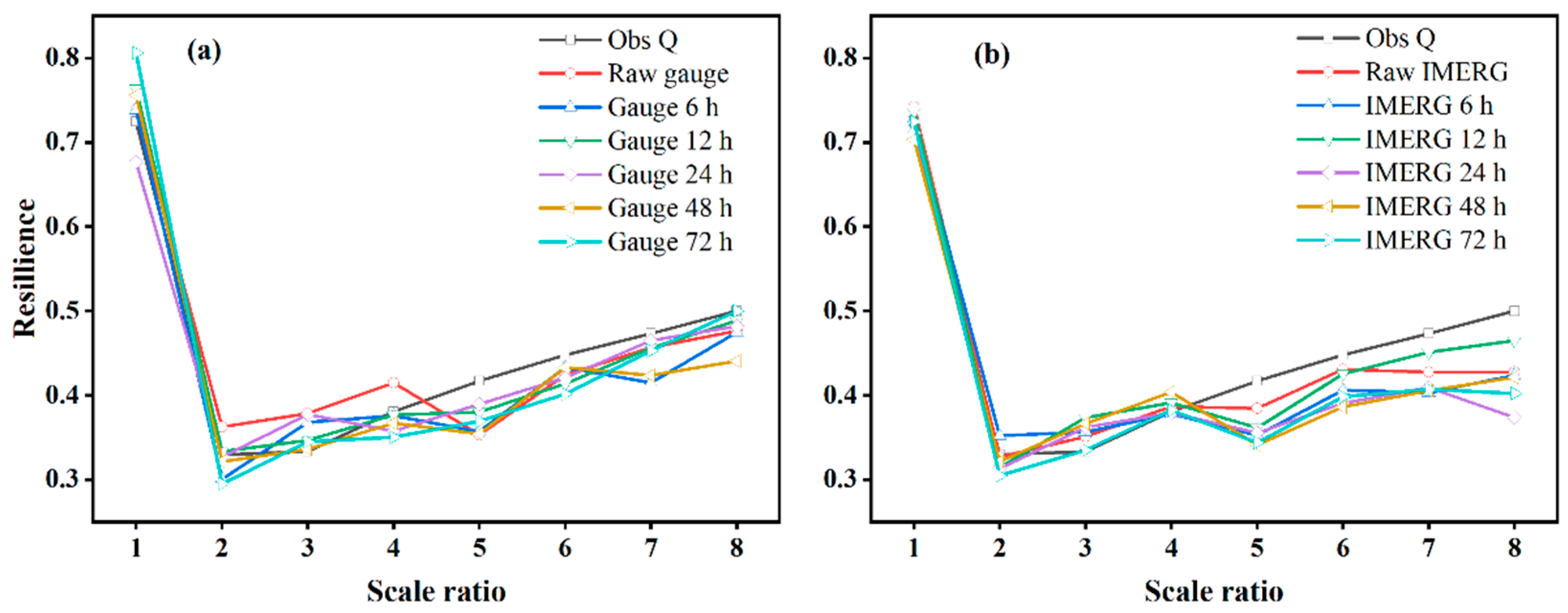
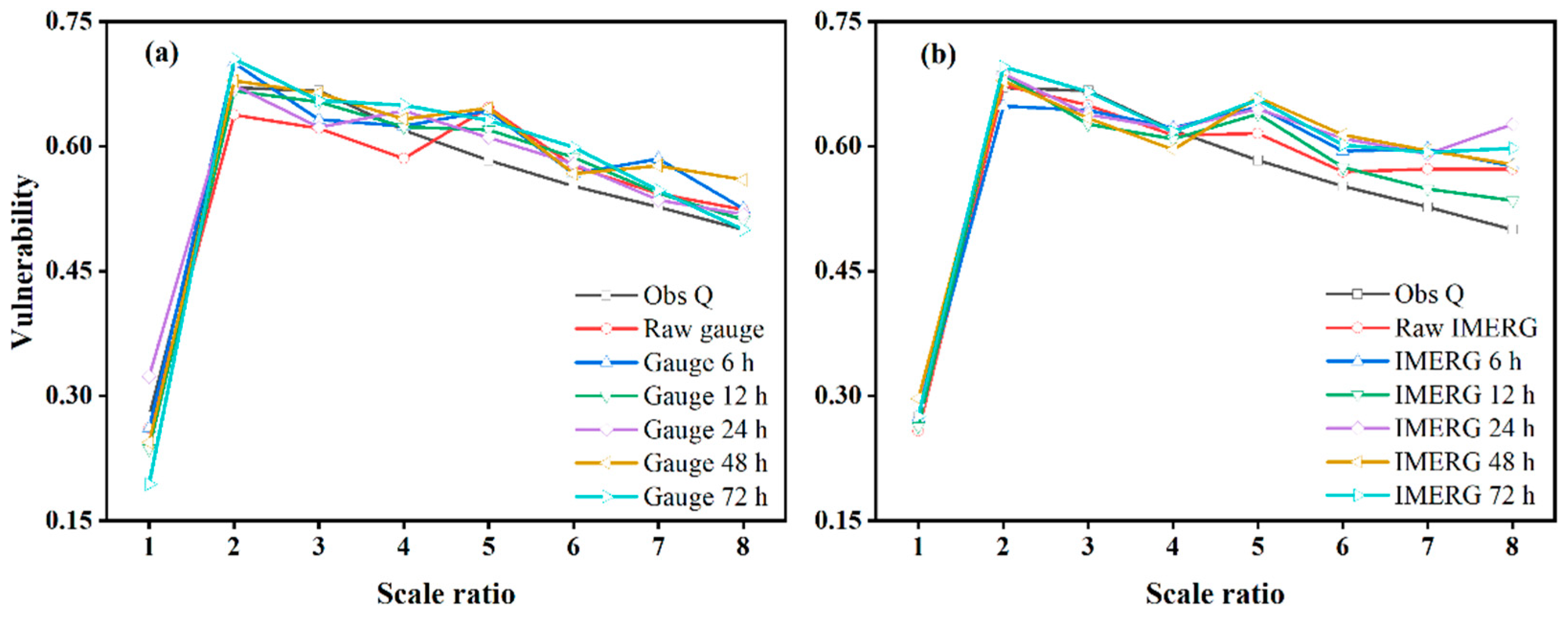
4.3.1. Analysis of rrv Indices

Analyzing the rrv indices of the optimal operation output with specific flood inflow forecast scenarios relative to IMERG and gauge rainfall can reveal the dynamical robustness change of the reservoir water supply function with the varying scale ratio. Figure 8 shows the reliability of water supply operation simulated with the flood inflow at five forecast lead times from sub-daily to daily scales. It clearly depicts that for the gauge rainfall case, the reliability value decreases in the first two states reaching bottom in the second state with maximum depth = 102 m and then increases from the second state. The reliability fluctuates in the range of 0.55–0.86 for the gauge rainfall-based flood inflow forecast cases over the eight states of scale ratio, which is significantly higher than the observed flood inflow case (0.53–0.82) for a specific scale ratio. Among five lead times, the trend in reliability curve with flood inflow at the 72 h lead time agrees best with the observed flood inflow, while this trend with flood flow at the 6 h lead time has the largest distance with the benchmark curve regarding the observed flood data. Among the eight states, the reliability values of forecasted flood inflow generated from state 1 of the scale ratio match the value of the observed flood inflow best for all the forecast lead times. The IMERG-based reservoir operation experiment produces a very similar trend and comparable values in magnitude of reliability to the gauge rainfall-based experiment for a specific lead time, with the only exception of a smaller value at the 6 h lead time in the scale ratio state 8.

For both gauge rainfall-based and IMERG-based flood inflow forecast cases, the resilience value of each lead time peaks in state 1 of the scale ratio (corresponding to the largest maximum depth of 103 m), while touching bottom in state 2 of the scale ratio (corresponding to the second largest maximum depth of 102 m, Figure 9). When the scale ratio state > 2, the resilience value of each lead time for both gauge rainfall-based and IMERG-based flood forecast experiments rises fluctuatingly, while this value of observed flood inflow data gradually increases. Furthermore, for each of the five lead times, the distance of resilience values between the IMERG-based flood inflow and the benchmark of the observed flood case is larger than that of the values between gauge rainfall-based flood inflow and the benchmark when the scale ratio state > 4, whereas this relation in magnitude of resilience between IMERG-based and gauge rainfall-based flood inflow forecast reverses when the scale ratio is in state 1.

The vulnerability and resilience indices have a complementary relationship, since the sum of these two values is equal to 1. Thereby, the vulnerability of all five lead times reaches the bottom in the scale ratio state 1, while appearing as the largest value in the scale ratio state 2 for both IMERG-based and gauge rainfall-based flood inflow forecast (Figure 10). For the majority of the combinations of the five lead times and eight scale ratio states, the vulnerability values related to IMERG data are slightly higher than those related to gauge-measured rainfall.

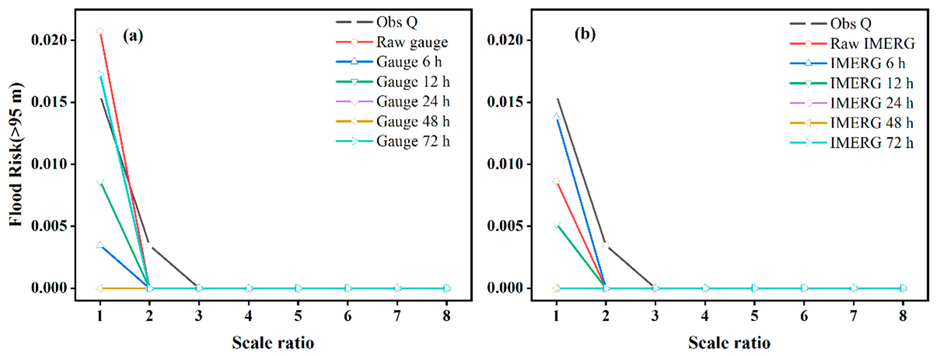
4.3.2. Analysis of Flood Risk Ratio Indices

For both the IMERG-based and gauge rainfall-based flood inflow forecast, the flood risk ratio at different lead times, which consider the regulated water level > 95 m, generally display a decrease with the varying scale ratio states. In a specific state of the scale ratio, the flood risk ratio derived from IMERG heavy rainfall at different lead times is significantly lower than that associated with the gauge heavy rainfall (Figure 11).

When choosing the threshold of water level as 96 m (Figure 12), the flood risk ratio is significantly smaller than that taking 95 m as the threshold in Figure 11. This flood risk ratio is greater than zero only in state 1 of the scale ratio and at the lead time of 72 h for the gauge rainfall-based case and for the observed flood inflow with values of 0.0034 and 0.0052, respectively (Figure 12a). As for the IMERG-related flood inflow forecast, the flood risk ratio in flood control operation is zero at various lead times (Figure 12b). For the threshold with 96 m, the flood risk ratio is zero across all the lead times and scale ratio states for both IMERG and gauge rainfall cases.

5. Discussion

The performance analysis mentioned above highlights a good general behavior of rrv indices related to flood inflow forecast at all the selected lead times. The rrv values between IMERG and gauge rainfall sources are comparable in trend, for a specific lead time. The impact of the scale ratio on rrv is not monotonous but with an inflection point. Specially, reservoir operation with the forecasted flood inflow via the IMERG and gauge rainfall in states 5 to 8 of the scale ratio generally obtained higher reliability and vulnerability, while having lower resilience and flood risk ratio values, compared with the actual flood inflow. For smaller reservoir scale, i.e., larger state number of the scale ratio, the IMERG-related rrv values fluctuate more dramatically than the gauge-related rrv values among varying lead times, indicating higher sensitivity of rrv to IMERG-related inflow forecast uncertainty. There is no consistent pattern in the magnitude of rrv among different lead times and between IMERG and gauge rainfall sources. In addition, the forecasted flood inflow at all lead times for both IMERG and gauge rainfall shows a much lower flood risk ratio (Figure 11 and Figure 12), compared with the actual flood inflow series. This also implies the positive impact of considering forecast uncertainty exerted on flood control operation. Furthermore, the flood risk ratio with IMERG forecast always exhibits lower values than that with gauge rainfall. This suggests the acceptable applicability of the IMERG heavy rainfall in flood control operation.

The uncertainty propagation from errors in stochastic generation of heavy rainfall, event-based flood inflow forecast, to the robustness of reservoir optimal operation shows different patterns between IMERG and gauge rainfall sources. This could be analyzed in detail as follows. First, each CDF curve at five forecast lead times for IMERG showed larger discrepancy to the raw IMERG CDF than that for the gauge rainfall data to the raw gauge CDF (Figure 5). This indicates significant forecast errors inherent in the synthetic forecast of IMERG heavy rainfall. Second, the CDF curves of forecast flood inflow at different lead times match well with the benchmark CDF of observed flood inflow series for both IMERG and gauge rainfall sources (Figure 7). This demonstrates that the hydrological process from heavy rainfall to event-based flood simulation reduces the initial heavy rainfall forecast error. Finally, the reservoir system in water supply and flood control operation using the IMERG-based flood inflow forecast even behaves better than that using the gauge rainfall-based flood inflow forecast at several lead times, and exerts either positive or negative impact on reservoir system robustness (Figure 8, Figure 9, Figure 10, Figure 11 and Figure 12). Additionally, the pattern of increasing forecast error of heavy rainfall with the lead time increasing can be generally observed from sub-daily to daily scales (see the CDF curves in Figure 5), whereas this pattern was not significant in the flood inflow forecast (Figure 7) and the dynamics of four risk-based robustness indices (Figure 8, Figure 9, Figure 10, Figure 11 and Figure 12). The intrinsic limitations of GPM constellation sensors in detecting heavy precipitation at the sub-daily temporal scales could reduce the consistency of the IMERG product and gauge heavy rainfall forecast. However, the rainfall–runoff model GR4H and reservoir optimal operation system could compensate the considerable gap between two precipitation sources and derive acceptable flood forecast and robust operation decision series of the Wan’an reservoir. This result conforms to the study conclusion of the previous study [12] that although the SPE products are not as accurate as the gauge rainfall, they could perform even better in streamflow simulations when combining with the appropriate hydrological model structure.

6. Conclusions

To assess the IMERG satellite precipitation-informed reservoir inflow forecast towards robust operation, a hypothetical case study was conducted by generating synthetic heavy rainfall forecast, flood inflow forecast of the reservoir, optimal operation outputs, and quantifying the risk-based robustness of reservoir system. The Wan’an reservoir and Wan’an basin were selected to be used in the case study, and the synthetic forecast of reservoir inflow was carried out based on event-based flood inflow series and varying lead times from sub-daily to daily scales. The primary conclusions are as follows:

(1)

The flood forecast with GR4H forced with IMERG shows slightly lower accuracy than that driven by the gauge rainfall of the Wan’an basin with the median r, NSE, KGE, and RMSE values ranging from 0.86–0.91, 0.67–0.75, 0.68–0.73, and 0.29 mm–0.33 mm for IMERG, respectively, and 0.88–0.91, 0.72–0.74, 0.64–0.77, and 0.26 mm–0.32 mm for gauge measured rainfall, respectively, across varying lead times.

(2)

For a specific robustness index, its trends between IMERG and gauge rainfall inputs are comparable, while its magnitude depends on varying lead times and scale ratios (i.e., the reservoir scale). The rrv values are more sensitive to IMERG-related rainfall and inflow forecast uncertainty for the smaller reservoir scale.

(3)

The pattern of increasing forecast error in rainfall with the lead time increasing is changed in the resultant inflow forecast series and dynamics of four risk-based robustness indices of optimal operation decision, due to the rainfall–runoff model and reservoir operation system partly compensating the original heavy rainfall forecast errors in IMERG and gauge data.

Our study highlights the acceptable hydrological applicability of IMERG rainfall towards the reservoir inflow forecast for robust operation despite the intrinsic error in SPE, motivating further cascading risk propagation investigation, from rainfall forecast uncertainty to operation risk.

References

1. Maggioni, V.; Massari, C. On the performance of satellite precipitation products in riverine flood modeling: A review. J. Hydrol. 2018, 558, 214–224. [Google Scholar] [CrossRef]
2. Pradhan, R.K.; Markonis, Y.; Godoy, M.R.V.; Villalba-Pradas, A.; Andreadis, K.M.; Nikolopoulos, E.I.; Papalexiou, S.M.; Rahim, A.; Tapiador, F.J.; Hanel, M. Review of GPM IMERG performance: A global perspective. Remote Sens. Environ. 2022, 268, 112754. [Google Scholar] [CrossRef]
3. Bitew, M.M.; Gebremichael, M. Assessment of satellite rainfall products for streamflow simulation in medium watersheds of the Ethiopian highlands. Hydrol. Earth. Syst. Sc. 2011, 15, 1147–1155. [Google Scholar] [CrossRef]
4. Wu, H.; Kimball, J.S.; Li, H.; Huang, M.; Leung, L.R.; Adler, R.F. A new global river network database for macroscale hydrologic modeling. Water Resour. Res. 2012, 48, W09701. [Google Scholar] [CrossRef]
5. Wang, Z.; Zhong, R.; Lai, C.; Chen, J. Evaluation of the GPM IMERG satellite-based precipitation products and the hydrological utility. Atmos. Res. 2017, 196, 151–163. [Google Scholar] [CrossRef]
6. Wang, C.; Tang, G.; Han, Z.; Guo, X.; Hong, Y. Global intercomparison and regional evaluation of GPM IMERG Version-03, Version-04 and its latest Version-05 precipitation products: Similarity, difference and improvements. J. Hydrol. 2018, 564, 342–356. [Google Scholar] [CrossRef]
7. Su, J.; Lü, H.; Zhu, Y.; Wang, X.; Wei, G. Component analysis of errors in four GPM-based precipitation estimations over Mainland China. Remote Sens. 2018, 10, 1420. [Google Scholar] [CrossRef]
8. Sui, X.; Li, Z.; Ma, Z.; Xu, J.; Zhu, S.; Liu, H. Ground Validation and Error Sources Identification for GPM IMERG Product over the Southeast Coastal Regions of China. Remote Sens. 2020, 12, 4154. [Google Scholar] [CrossRef]
9. Pradhan, R.K.; Markonis, Y. Performance evaluation of GPM IMERG precipitation products over the tropical oceans using Buoys. J. Hydrometeorol. 2023, in press. [CrossRef]
10. Gentilucci, M.; Barbieri, M.; Pambianchi, G. Reliability of the IMERG product through reference rain gauges in Central Italy. Atmos. Res. 2022, 278, 106340. [Google Scholar] [CrossRef]
11. Moazami, S.; Na, W.; Najafi, M.R.; de Souza, C. Spatiotemporal bias adjustment of IMERG satellite precipitation data across Canada. Adv. Water. Resour. 2022, 168, 104300. [Google Scholar] [CrossRef]
12. Qi, W.; Zhang, C.; Fu, G.T.; Sweetapple, C.; Zhou, H.C. Evaluation of global fine-resolution precipitation products and their uncertainty quantification in ensemble discharge simulations. Hydrol. Earth. Syst. Sc. 2016, 20, 903–920. [Google Scholar] [CrossRef]
13. Ali, M.; Amir, A.K. Capabilities of satellite precipitation datasets to estimate heavy precipitation rates at different temporal accumulations. Hydrol. Process. 2014, 28, 2262–2270. [Google Scholar]
14. Sharifi, E.; Steinacker, R.; Saghafian, B. Multi time-scale evaluation of high-resolution satellite-based precipitation products over northeast of Austria. Atmos. Res. 2018, 206, 46–63. [Google Scholar] [CrossRef]
15. Simanjuntak, F.; Jamaluddin, I.; Lin, T.-H.; Siahaan, H.A.W.; Chen, Y.-N. Rainfall Forecast Using Machine Learning with High Spatiotemporal Satellite Imagery Every 10 Minutes. Remote Sens. 2022, 14, 5950. [Google Scholar] [CrossRef]
16. Yue, H.; Gebremichael, M.; Nourani, V. Performance of the Global Forecast System’s medium-range precipitation forecasts in the Niger river basin using multiple satellite-based products, Hydrol. Earth Syst. Sci. 2022, 26, 167–181. [Google Scholar] [CrossRef]
17. Dobson, B.; Wagener, T.; Pianosi, F. An argument-driven classification and comparison of reservoir operation optimization methods. Adv. Water Resour. 2019, 128, 74–86. [Google Scholar] [CrossRef]
18. Lu, Q.; Zhong, P.; Xu, B.; Zhu, F.; Ma, Y.; Wang, H.; Xu, S. Risk analysis for reservoir flood control operation considering two-dimensional uncertainties based on Bayesian network. J. Hydrol. 2020, 589, 125353. [Google Scholar] [CrossRef]
19. Herbert, Z.C.; Asghar, Z.; Oroza, C.A. Long-term reservoir inflow forecasts: Enhanced water supply and inflow volume accuracy using deep learning. J. Hydrol. 2021, 601, 126676. [Google Scholar] [CrossRef]
20. Ahmad, S.K.; Hossain, F. A generic data-driven technique for forecasting of reservoir inflow: Application for hydropower maximization. Environ. Modell. Softw. 2019, 119, 147–165. [Google Scholar] [CrossRef]
21. Yang, S.; Yang, D.; Chen, J.; Zhao, B. Real-time reservoir operation using recurrent neural networks and inflow forecast from a distributed hydrological model. J. Hydrol. 2019, 579, 124229. [Google Scholar] [CrossRef]
22. Meydani, A.; Dehghanipour, A.; Schoups, G.; Tajrishy, M. Daily reservoir inflow forecasting using weather forecast downscaling and rainfall-runoff modeling: Application to Urmia Lake basin, Iran. J. Hydrol. Reg. Stud. 2022, 44, 101228. [Google Scholar] [CrossRef]
23. Prakash, S.; Mitra, A.K.; AghaKouchak, A.; Liu, Z.; Norouzi, H.; Pai, D.S. A preliminary assessment of GPM-based multi-satellite precipitation estimates over a monsoon dominated region. J. Hydrol. 2018, 556, 865–876. [Google Scholar] [CrossRef]
24. Tang, G.; Clark, M.P.; Papalexiou, S.M.; Ma, Z.; Hong, Y. Have satellite precipitation products improved over last two decades? A comprehensive comparison of GPM IMERG with nine satellite and reanalysis datasets. Remote Sens. Environ. 2020, 240, 111697. [Google Scholar] [CrossRef]
25. Huffman, G.J.; Bolvin, D.T.; Braithwaite, D.; Hsu, K.; Joyce, R.; Kidd, C.; Nelkin, E.J.; Sorooshian, S.; Tan, J.; Xie, P. NASA Global Precipitation Measurement (GPM) Integrated Multi-Satellite Retrievals for GPM (IMERG); Algorithm Theoretical Basis Document (ATBD) Version, 06; NASA/GSFC: Greenbelt, MD, USA, 2018; 39p. [Google Scholar]
26. He, X.; Chaney, N.W.; Schleiss, M.; Sheffield, J. Spatial downscaling of precipitation using adaptable random forests. Water Resour. Res. 2016, 52, 8217–8237. [Google Scholar] [CrossRef]
27. Van Esse, W.R.; Perrin, C.; Booij, M.J.; Augustijn, D.C.; Fenicia, F.; Kavetski, D.; Lobligeois, F. The influence of conceptual model structure on model performance: A comparative study for 237 French catchments. Hydrol. Earth Syst. Sci. 2013, 17, 4227–4239. [Google Scholar] [CrossRef]
28. Perrin, C.; Michel, C.; Andréassian, V. Improvement of a parsimonious model for streamflow simulation. J. Hydrol. 2003, 279, 275–289. [Google Scholar] [CrossRef]
29. Zhang, Y.; Vaze, J.; Chiew, F.H.; Teng, J.; Li, M. Predicting hydrological signatures in ungauged catchments using spatial interpolation, index model, and rainfall–runoff modelling. J. Hydrol. 2014, 517, 936–948. [Google Scholar] [CrossRef]
30. Haruna, A.; Garambois, P.; Roux, H.; Javelle, P.; Jay-Allemand, M. Signature and sensitivity-based comparison of conceptual and process oriented models, GR4H, MARINE and SMASH, on French Mediterranean flash floods. Hydrol. Earth Syst. Sci. Discuss. 2021. preprint. [Google Scholar] [CrossRef]
31. Basri, H.; Sidek, L.M.; Razad, A.Z.; Pokhrel, P. Hydrological Modelling of Surface Runoff for Temengor Reservoir Using GR4H Model. Int. J. Civ. Eng. Technol. 2019, 10, 22–28. [Google Scholar]
32. Turner, S.W.; Galelli, S. Water supply sensitivity to climate change: An R package for implementing reservoir storage analysis in global and regional impact studies. Environ. Model. Softw. 2016, 76, 13–19. [Google Scholar] [CrossRef]
Figure 1. Location of the Wan’an basin, and distribution of rain stations, stream network, and the DEM in this basin.
Remotesensing 15 04741 g001
Figure 2. Schematic framework of this study.
Remotesensing 15 04741 g002
Figure 3. Scatters of forecasted IMERG and gauge rainfall vs. the raw gauge rainfall at each lead time of (a) 6 h, (b) 12 h, (c) 24 h, (d) 48 h, and (e) 72 h and (f) 0 h (the “Raw” data).
Remotesensing 15 04741 g003
Figure 4. Probability density function (PDF) of 6-hourly precipitation with different intensities, as derived from the raw and the forecasted IMERG and gauge precipitation in 31 storm events during 2014 and 2019 over the Wan’an basin.
Remotesensing 15 04741 g004
Figure 5. Cumulative distribution function (CDF) of 6-hourly precipitation as derived from the raw and the forecasted (a) gauge and (b) IMERG precipitation in 31 storm events during 2014 and 2019 over the Wan’an basin. Note: the “Raw” represents the raw gauge rainfall and IMERG data.
Remotesensing 15 04741 g005
Figure 6. Change in (a) r, (b) NSE, (c) KGE, and (d) RMSE indices of GR4H-forecasted flood Q with IMERG and gauge rainfall input over 31 storm-flood events occurring in the Wan’an basin during the period 2014–2019. The box and whisker plot (i.e., box plot) used here displays the five-number summary of a set of gauge rainfall-driven (in yellow) and IMERG satellite rainfall-driven (in purple) flood modeling series. The five-number summary is the minimum, first quartile, median, third quartile, and maximum of modeled flood data. The box from the first quartile to the third quartile is plotted and a vertical line goes through the box at the median.
Remotesensing 15 04741 g006
Figure 7. CDF curves of flood derived by rainfall–runoff model GR4H driven by the raw and forecasted (a) gauge and (b) IMERG rainfall over the Wan’an basin. Note: “Obs Q” and “Raw” denote CDF curves with the actual flood data and the simulated flood driven by the raw IMERG and gauge rainfall, respectively.
Remotesensing 15 04741 g007
Figure 8. Reliability dynamics with the varying scale ratio for (a) the gauge rainfall-based and (b) the IMERG-based flood inflow forecast (the scale ratio represents a factor that controls the change of reservoir states about capacity, maximum depth, and maximum surface).
Remotesensing 15 04741 g008
Figure 9. Resilience dynamics with the varying scale ratios for (a) the gauge rainfall-based and (b) the IMERG-based flood inflow forecast.
Remotesensing 15 04741 g009
Figure 10. Vulnerability dynamics with the varying scale ratio for (a) the gauge rainfall-based and (b) the IMERG-based flood inflow forecast.
Remotesensing 15 04741 g010
Figure 11. Flood risk ratio (>95 m) with the varying scale ratio for (a) the gauge rainfall-based and (b) the IMERG-based flood inflow forecast.
Remotesensing 15 04741 g011
Figure 12. Flood risk (>96 m) with the varying scale ratio states for (a) the gauge rainfall-based and (b) the IMERG-based flood inflow forecast.
Remotesensing 15 04741 g012