2.3.1. Calculation of Remote Sensing and Meteorological Drought Indices
Drought indices are critical for drought monitoring and prediction, serving as a prerequisite for accurate assessment. Each drought index possesses distinct features. Among remote sensing drought indices, the NDVI and EVI can be used for drought monitoring because they reflect the vegetation status. The TRMM-standardized precipitation index (TRMM-SPI) captures precipitation distribution and abnormalities in the study area. VCI is derived from the NDVI and minimizes season-related noises. The TCI is derived from LST and reflects surface sensible heat flux because stomatal closure in vegetation due to drought leads to increased sensible heat flux [
54]. The NDVI contains atmospheric noises, whereas the EVI inherits the advantages of the NDVI and overcomes some defects associated with the NDVI, including sensitivity to soil background effects, oversaturation of the NDVI in areas with high-rank vegetation cover, and reliance on atmospheric correction. In addition, the EVI is more sensitive to vegetation than the NDVI and therefore increases the sensitivity of vegetation monitoring. The EVI usually performs better when applied to vegetation degradation monitoring and quantitative analysis of vegetation resources [
55]. In this study, we calculated the VCI and TCI and estimated the VTCI, TVDI, and vegetation supply water index (VSWI) based on the NDVI, LST, and EVI, respectively. Both the VTCI and TVDI were calculated based on the triangular relationship between the VCI and LST. They reflected surface evapotranspiration by capturing the changes in the LST and thereby identifying drought occurrence by estimating the changes in the SM content. The VSWI was calculated from the LST and VCI and predicted drought occurrence in the case of an increase in leaf canopy temperature and a decrease in photosynthesis [
54].
Among meteorological drought indices, the SPEI considers both precipitation and potential evapotranspiration based on the water balance model of the SPI. The SPEI describes the multiscale features of a drought system. It is particularly suitable for drought study in the climate change context because it is subjected to fewer restrictions in geographical and climatic conditions [
16]. The MCI, developed by the National Climate Center by integrating several drought indices, has already been used in China’s meteorological businesses [
56]. In the present study, we used preprocessed remote sensing data and weather station observation data to calculate the VCI, TCI, VTCI
NDVI, VTCI
EVI, TVDI
NDVI, TVDI
EVI, VSWI
NDVI, VSWI
EVI, TRMM-SPI, SPEI, and MCI. The indices were used as input and output parameters for the ML model and served as a means to validate the performance of the model in assessing drought. The calculation formulas for the selected remote sensing drought indices and meteorological drought indices are presented in
Table 1.
The drought grades of SPEI and MCI values calculated based on the meteorological station data were consistent, as shown in
Table 2. SPEI1, SPEI3, and SPEI6 represent the SPEI values of the 1-month scale, 3-month scale, and 6-month scale, respectively.
2.3.2. ML Model
- (1)
RF Model
The RF model was proposed by Breiman (2001) and is based on CART, which is one of the DT algorithms [
62]. The rule-based ML, including decision trees and RF, has been widely used in remote sensing applications [
19,
34,
40,
63,
64,
65]. The RF method uses an ensemble approach that combines multiple decision trees to make predictions. The name “random forest” refers to data prediction accomplished using many independent DTs (a “forest”) through randomly selected training samples and variables at each node, which alleviates the well-known problems of CART such as overfitting and sensitivity to training data [
66]. A randomly selected subset of training samples is used to produce a tree. The final decision from multiple trees is made by aggregating individual tree results based on an averaging approach for regression or a majority voting for classification. The RF model calculates the increased percentage of mean square error using the out-of-bag data when a variable is permuted with a random value [
62]. Based on this information, the relative importance of a variable (i.e., the contribution of the variable to predict a target variable) can be identified. Therefore, RF can decrease the variance and obtain more precise prediction results than the common tree-based algorithms.
Let D be a training dataset in an M-dimensional space X, and let Y be the class feature with the total number of c distinct classes. The construction of an RF involves a three-step process [
62,
66]:
Step 1: Training data sampling: Use the bagging method to generate the K subsets of training data {D1, D2,..., DK} by randomly sampling D with replacement;
Step 2: Feature subspace sampling and tree classifier building: For each training dataset Di (1 ≤ i ≤ K), use a DT algorithm to grow a tree. At each node, randomly sample a subspace Xi of F features (F << M), compute all splits in subspace Xi, and select the best split as the splitting feature to generate a child node. Repeat this process until the stopping criteria are met, and a tree HI (Di, Xi) built by training data Di under subspace Xi is thus obtained;
Step 3: Decision aggregation: Ensemble the K trees {h1 (D1, X1), h2 (D2, X2), …, hK (DK, XK)} to form an RF and use the majority vote of these trees to make an ensemble classification decision.
The algorithm has two key parameters, i.e., the number of K trees to form an RF and the number of F randomly sampled features for building a DT. According to Breiman [
62], parameter K can be set to 100 and parameter F can be computed by F = [log2 M + 1]. For large and high-dimensional data, larger values of K and F should be used.
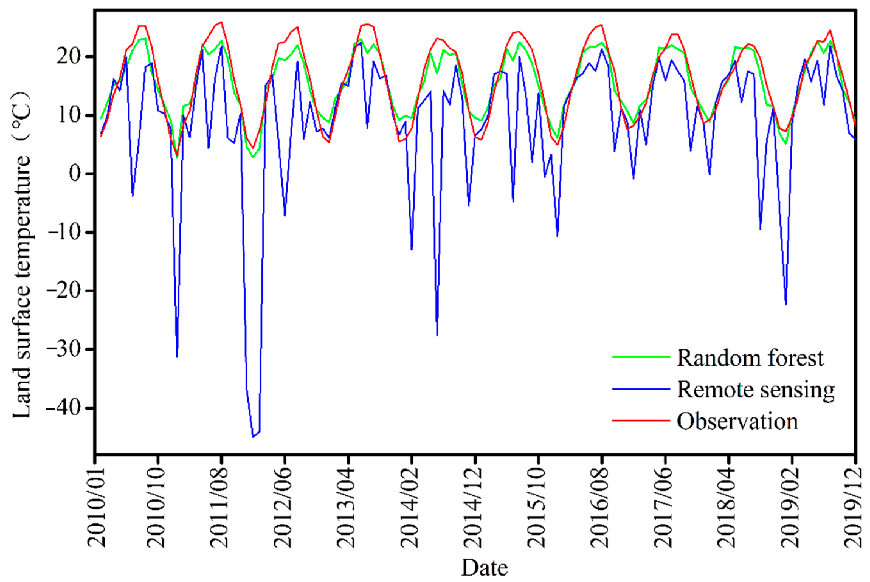
The LST is an important parameter characterizing land surface energy and water balance and is closely related to the SM content. It plays a crucial role in drought monitoring and prediction. In the feature space of vegetation index-LST (VI-LST), the LST value directly affects the distribution of data points on a scatterplot. This further affects the results of remote sensing inversion of drought indices, as shown in
Table 1, including TCI, VTCI, TVDI, and VSWI. However, the following three problems usually exist for the MODIS LST products: (1) The MODIS sensor passes over any given region four times a day with a fixed transit time. Therefore, the sensor cannot acquire data for a given region throughout the day or at a specified time. (2) Given the large differences in climate and topography across the regions, the accuracy of MODIS LST products fluctuates significantly. (3) In the presence of cloud cover, it is the cloud top temperature rather than the LST that is actually observed [
67]. We discovered during the preprocessing of MODIS LST data that the LST_Day and LST_Night data of MOD11A2 and MYD11A2 contained a large number of missing and error values, implying significant data errors.
RF in ML is an ensemble learning algorithm that uses a DT as the base learner and is considered highly accurate. An introduction of a tree ensemble endows RF with the ability to process nonlinear data and handle default values and data anomalies. Even if some of the features are already lost, RF may still ensure accuracy in monitoring and prediction. In addition, RF is relatively simple to implement and can balance the errors between datasets. Xiao et al. (2021) [
68] proposed an improved LST reconstruction method for cloud-covered pixels by building a linking model for the MODIS LST with other surface variables based on an RF regression method. The validation with in situ observations revealed that the reconstructed cloud-covered LSTs performed similarly to the LSTs on clear-sky days with correlation coefficients of 0.92 and 0.89, respectively. The unbiased
RMSE was calculated to be 2.63 K. Chen et al. (2020) [
69] also proposed a novel algorithm based on RF to reconstruct MODIS LST. The experimental results indicated that the algorithm had the capacity to enhance the estimation of MODIS LST products in terms of accuracy and data availability. Sun et al. (2023) [
70] used the RF model to produce a set of high-quality NDVI products to represent actual surface characteristics more accurately and naturally. Notably, the RF algorithm exhibited a
MAE of 0.024 and a
RMSE of 0.034, besides a
R2 value of 0.974. To effectively address the issue of significant blank areas resulting from frequent cloud cover in current thermal infrared-based LST products, Zhao et al. (2020) [
71] introduced a novel method for reconstructing the cloud-covered LSTs of Terra MODIS daytime observations using the RF regression approach. They applied the RF regression approach in southwestern Europe. The reconstructed LSTs showed similar spatial patterns compared with clear-sky LSTs from temporally adjacent days, demonstrating a stable and reliable performance. Wang et al. (2020) [
72] indicated that RF was superior to SVM and ANN in reconstructing and supplementing missing data.
Therefore, in the present study, we first reconstructed and supplemented the missing LST data using a built RF model and multiple impact factors related to remotely sensed LST monitoring, aiming to improve the precision of the MODIS LST products.
- (2)
XGBoost Model
The XGBoost model is an ensemble learning algorithm proposed by Chen and Guestrin (2016) [
73]. It is an ML technique designed for regression and classification tasks. It constructs a prediction model in the form of an ensemble of weak prediction models. As an efficient and scalable variant of the gradient boosting machine, XGBoost has recently won several ML competitions based on its convenience, parallelism, and impressive predictive accuracy [
74]. It is based on a gradient boosting decision tree (GBDT) and further optimizes performance by improving the model to fit the target and adding regularization terms to the objective function. The GBDT algorithm uses only the first-order derivative information for optimizing the loss function, whereas the XGBoost algorithm performs a second-order Taylor expansion of the loss function. By incorporating both the first- and second-order derivative information, XGBoost achieves a better fit to the loss function and reduces errors during the optimization process. The specific definition is provided as follows [
64,
75,
76].
Given a training dataset D = {(x
1, y
1), (x
2, y
2),…, (x
n, y
n)}, x
i ∈ X ⊆ R
m, y
i ∈ Y ⊆ R, X is the input space, and Y is the output space. XGBoost can be expressed as an additive model as follows:
where
represents the predicted value of the training model,
represents the
kth submodel; and
represents the
ith input sample. The optimization objectives of the XGBoost algorithm include a loss function and a regularization term, and the final optimization objectives can be determined as:
where
represents the objective function at the
tth iteration;
represents the class-label of the original sample;
represents the predicted value of the model during t – 1 model iterations of the sample;
) represents the predicted value of the model during the
tth model iteration of the sample; and
is the regularization term of the objective function. The Taylor expansion of Equation (2) yields:
where
represents the first-order gradient of the sample
;
represents the second-order gradient of the sample
;
represents the output value of the
jth node;
and
are the coefficients of the regularization term to prevent the model from overfitting; and
is the subset of samples in the
jth leaf node.
The training process of the XGBoost model was used to solve Equation (3) and find the best
and the optimal solution of the corresponding objective function:
Equation (5) was used to measure the quality of a tree structure; the lower the value, the better the tree structure. Therefore, when the nodes in the tree were split, Equation (6) was obtained as follows:
If the gain value is greater than zero, the node splitting continues; otherwise, the node splitting stops.
The RF algorithm can properly handle missing and abnormal values, but it tends to neglect the correlations between the attributes, thereby affecting the regression performance. Therefore, in the present study, a remote sensing drought monitoring model was constructed based on the multisource remote sensing information (multiple remote sensing drought indices involved), and we reconstructed the LST using the RF model and XGBoost. The rationale for selecting the XGBoost model was as follows:
- (A)
XGBoost belongs to the category of rule-based models. Those models are generally better suited than DL algorithms for the datasets of moderate or small size.
- (B)
XGBoost models have a higher accuracy due to the introduction of second-order Taylor expansion. The base learner of XGBoost can be a DT or a linear classifier, implying higher flexibility.
- (C)
XGBoost models are convenient to build in that they can attain highly optimized performance by following a standard hyperparameter search process implemented using stratified k-fold nested cross-validation (CV). Because of the regularization term, XGBoost can also be easily trained in such a way as to reduce overfitting.
- (D)
XGBoost can incorporate elements of cost-sensitive learning where a cost matrix can help influence the model to produce fewer false negatives.
- (E)
XGBoost supports column sampling, and it can reduce computational load and accelerate the calculation. It has been used successfully to win several ML competitions.
- (F)
Previous drought studies have obtained successful results using XGBoost for predicting meteorological indicators [
74,
76,
77].
2.3.3. CV Method
A central tenet of accuracy assessment is that the samples used for training should not also be used for evaluation. A similar concern applies to the methods for selecting the user-specified parameters required by most ML methods. The value of these parameters can affect the accuracy of the classification, and thus, the optimization of the chosen values (sometimes called tuning) is usually required [
78,
79,
80,
81,
82]. Tuning is generally empirical, with various values for the parameters systematically evaluated, and the combination of values that generate the highest overall accuracy is assumed to be optimal [
80,
83]. Excluding training samples from the samples used for evaluating the candidate parameter values reduces the likelihood of overtraining and thus improves the generalization of the classifier.
CV is an approach used for exploiting training and accuracy assessment samples multiple times and thus potentially improving the reliability of the results. It can also have a better effect on small sample data. CV involves the creation of multiple partitions, potentially allowing each sample to be used multiple times for multiple purposes, with the overall aim of improving the statistical reliability of the results. Various CV methods exist, including
k-fold, leave-one-out, and Monte Carlo. Classification parameter tuning via CV has been demonstrated to improve classification accuracy in remote sensing analyses [
84].
The
k-fold CV method involves randomly splitting the sample set into a series of equally sized folds (groups), where
k indicates the number of partitions or folds the dataset is split into. For example, if a
k-value of five is used, the dataset is split into five partitions. In this case, four of the partitions are used for training data, while the remaining one partition is used for validation data. The training process is repeated five times, with each iteration using a different partition as the validation set and the remaining four partitions as the training data. The average of the results is then reported [
85]. Some studies showed the merits of the cross-validation methods such as
k-fold CV for parameter tuning [
80,
82,
83], and the optimal value for
k should be 5 or 10 to avoid issues associated with imbalanced datasets [
86]. To improve the generalization, robustness, and reliability of the constructed models, we employed a 5-fold CV method to fine-tune the models’ hyperparameters in the present study.
2.3.4. Indicators of Model Accuracy Assessment
Because the evaluation indicators of regression tasks mainly focus on the differences between predicted and true values, the accuracy of the two models was evaluated by computing and comparing statistical measures based on the differences between the observed (114 weather stations) and predicted (LST and SPEI) values. These metrics included
CC,
RMSE,
MAE, and
EVS, which were calculated using Equations (7)–(10), respectively.
where
i is the data of the
ith sample point,
refers to the true value of the sample,
refers to the predicted value of the sample, and
and
refer to the average of the true value sample and predicted value sample, respectively. The
n symbol refers to the number of samples, and
Var is the sample variance. Among the five indicators,
CC is used to measure the correlation between the two variables. The value of
CC is between −1 and 1; the closer its value is to 1 or −1, the stronger the relationship between the true value and the predicted value. The
EVS is between 0 and 1. The closer its value is to 1, the better the model effect. The
RMSE is the deviation between the predicted value and the true value. It is often used as a standard for measuring the prediction results of ML models. The value of
RMSE and
MAE is between 0 and ∞; they are two indices greater than zero, and the closer its value is to 0, the better the model effect [
65,
73].
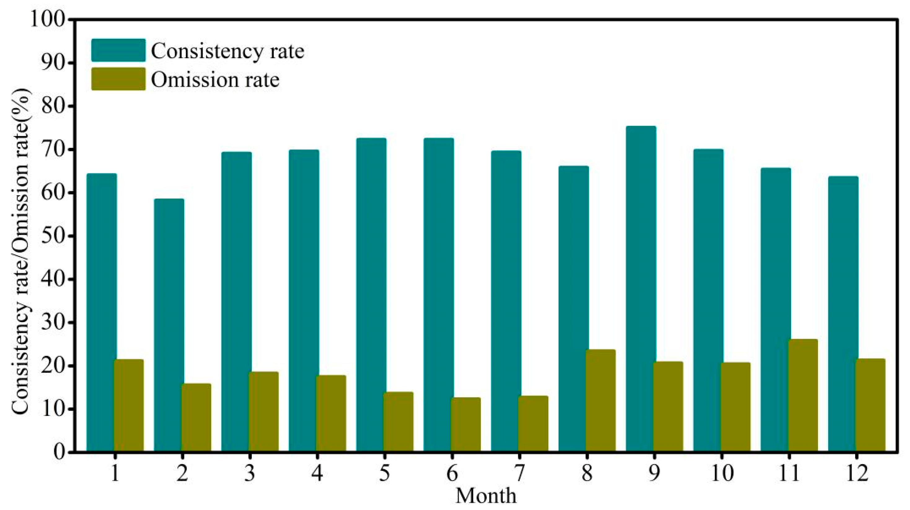
In addition, by classifying drought grades from the model-predicted and station-calculated SPEI values (
Table 2), the consistency rate and omission rate were also used to evaluate the model accuracy in our study. The consistency rate is the ratio of the number of correctly classified samples to the total number of samples for a given dataset. The omission rate is the percentage of weather stations where no drought occurred based on monitoring values from the model to all of the weather stations where drought was considered to occur based on the estimated values of the drought index. The calculation formula for both cases is as follows [
87,
88].
where
CS is the number of weather stations correctly classified by drought grade (the classification of the drought index output by the model is consistent with the classification of the drought index estimated by the meteorological station according to
Table 2),
O is the total number of weather stations belonging to this drought grade,
NR is the number of weather stations where no drought occurred based on model monitoring, but the corresponding reality is drought, and
T is the total number of weather stations with actual drought conditions.


