Construction and Analysis of the EMC Evaluation Model for Vehicular Communication Systems Based on Digital Maps

Abstract

With the development of vehicular communication technology, the electromagnetic compatibility requirements of vehicular communication systems are becoming more demanding. The traditional four-level electromagnetic compatibility evaluation model is widely applied in many scenarios. However, this model neglects the mutual interference of electronic devices inside a vehicle, and it cannot evaluate whether reduced radio receiver sensitivity, antenna isolation, and communication distance satisfy the system requirements for vehicular communication, thus making it unsuitable for digital communication systems. With the development of remote sensing technology, high-precision digital maps are easy to acquire and thus widely used. In this work, a modified five-level evaluation model based on digital maps is proposed, where digital maps are employed to support receiver sensitivity, antenna isolation, and communication performance evaluation. Through remote sensing technology and digital maps, a terrain profile is obtained, and a more accurate vehicle communication propagation model is established. In the experiment, an actual armored vehicular communication system example is applied to verify the performance of the proposed five-level evaluation model. Compared with the free-space propagation model, the error of the actual power received by the receiver is reduced by 0.97%, and the error of the communication distance where the sensitivity of the receiver is reduced by more than the system EMC threshold is reduced by 16.78%. The calculated antenna isolation degree is basically consistent with the actual measurement data. The model is able to evaluate the electromagnetic compatibility of an armored vehicular communication system more quickly, accurately, and comprehensively compared to previous evaluation models.

1. Introduction

With the prevailing tendency of integrating an extensive range of electronic devices into vehicles, the electromagnetic environments of vehicular communication systems have grown increasingly intricate. The intensity of electromagnetic interference (EMI) amplifies in correlation with the complexity of the electromagnetic environment [1,2,3,4,5,6,7,8]. EMI stands out as the principal factor contributing to electromagnetic compatibility (EMC) issues [9,10,11,12,13]. It is responsible for various complications, including diminished communication quality and the disruption of regular communication processes. Several EMC evaluation models have been proposed, including the ACAT model [14,15], the IEMCAP model [16,17], and the IAP model [18]. Recently, a modified four-level evaluation model was proposed [19]. The traditional four-level evaluation model is widely regarded as one of the most enduring and frequently employed models in the field [20]. The design of the traditional four-level assessment model can be broken down into four hierarchical levels. By first performing a rough assessment based on the signal amplitude, the least likely potential EMI sources can be eliminated directly. Next, the second-level EMC assessment is performed based on spectral analysis, and detailed prediction and performance analyses are performed as the third and fourth levels of the EMC assessment process.

However, due to advancements in vehicular electronic technology, the conventional model has become restricted, antiquated, and inadequate, particularly concerning armored vehicular communication systems. The traditional four-level evaluation model exhibits several limitations when employed in the evaluation of electromagnetic compatibility within armored vehicular communication systems:

(1) The potential mutual interference caused by the simultaneous operation of multiple electronic devices is not taken into consideration.

(2) An evaluation of whether the decreased isolation between antennas meets the electromagnetic compatibility requirements of a system is not performed when vehicle-mounted antennas are functioning simultaneously.

(3) An evaluation of whether the reduced sensitivity of the radio receiver meets the electromagnetic compatibility requirements of a system is not conducted.

(4) The impact of the actual terrain environment on the communication distance is not investigated.

(5) The evaluation criteria used for evaluating vehicular communication quality are overly simplistic and unsuitable for digital communication systems.

In recent years, remote sensing technology has developed rapidly and is now widely used, e.g., LiDAR localization technology [21,22,23,24]. Since high-precision digital maps are easy to acquire, they are widely used in wireless communication [25,26,27,28]. The communication distance and quality of a vehicular communication system are easily affected by complex terrain and geomorphology factors, thus increasing radio wave propagation loss and seriously affecting communication performance. In light of the progress in this field, it has become imperative to tackle the aforementioned issue by developing an evaluation model that aligns with the specific characteristics of armored vehicular communication systems and the application of digital maps. Therefore, in this paper, we introduce a modified five-level evaluation model, which is based on digital maps, for conducting EMC evaluations of armored vehicular communication systems. The reduction in the sensitivity of a radio receiver is directly determined by the actual power it receives, wherein the path loss of radio propagation plays a critical role in influencing both the actual power received by the radio receiver and the achievable communication distance. Digital maps are extremely intuitive and accurate tools for obtaining geographical information, including vehicle distances, terrain surface, terrain height, and land cover. Such information plays a crucial role in determining the path loss of radio wave propagation. Consequently, utilizing digital maps in the evaluation of receiver sensitivity and communication performance can enhance the accuracy of the results. The main contributions of this article are as follows.

(1) According to the developed digital map, a terrain profile and a contour map are obtained. The vehicle communication system propagation model is established based on the actual terrain. Through the above propagation model, the power received by the receiver and the reduction in the receiver’s sensitivity are calculated. The correctness of the evaluated model is verified in comparison with the free-space propagation model and the measured data.

(2) Using the actual terrain propagation model of the vehicle communication system, the isolation between the vehicle-mounted antennas is calculated. Compared with the measured data, the correctness of the evaluation model is verified.

(3) The decreases in the communication distances of the vehicle communication system under a free-space propagation model and an actual terrain propagation model are analyzed and compared.

The remainder of this paper is structured as follows. Section 2 provides a succinct introduction to the theoretical mechanism of EMI. Section 3 presents the modified five-level evaluation model for armored vehicular communication systems, encompassing the model’s architecture, evaluation components, methodologies, and criteria for each level. To validate the proposed model, Section 4 utilizes an example of an armored vehicular communication system. In Section 5, the performance of the proposed model is discussed. Finally, Section 6 concludes the paper by summarizing the key findings and implications.

2. EMI Theoretical Mechanism

In practical cases, a vehicular communication system usually includes several electronic devices, such as HF radios, VHF radios, and other devices. The mutual influence of these devices will inevitably lead to complex electromagnetic environments in these systems and may generate various types of EMI, such as fundamental wave interference, high-order harmonic wave interference, and high-order intermediation interference [29,30].

Assuming that the original transmitted signal in the system is $s(t)$, it is expressed as in Equation (1). Because of the mutual influence among the electronic devices in the system, $s(t)$ is subjected to the mutual effect gain $G[s(t)]$, and its form is shown in Equation (2), where $a_i$ denotes the power coefficients of the devices. Under the mutual influence of $G[s(t)]$, $s(t)$ can be modified to $u(t)$, as expressed in Equation (3).

$$s(t)=A\cos ({\omega }_{1}t)+B\cos ({\omega }_{2}t)$$

(1)

$$G[s(t)]={\displaystyle \sum _{i=1}^{\infty }{a}_i{s}^{i-1}(t)} i=1,2,3\dots$$

(2)

$$u(t)=s(t)G\left[s(t)\right]$$

(3)

By taking the power series expansion of $u(t)$ in terms of $s(t)$, the final signal can be expressed as the sum of various additional signal components, which is shown in Equation (4) and

Table 1. The main additional components of the signal.

Formula	Signal Component
$A\cos ({\omega }_{1}t)+B\cos ({\omega }_{2}t)$	original signal
$a_1[A\cos ({\omega }_{1}t)+B\cos ({\omega }_{2}t)]$	fundamental wave
$a_{2}AB[A\cos ({\omega }_1+{\omega }_2)t+B\cos ({\omega }_1-{\omega }_2)t]$	second-order intermediation
$a_2[A^2\cos (2{\omega }_{1}t)+B^2\cos (2{\omega }_{2}t)]/2$	second-order harmonic wave
$3a_3{A}^{2}B[\cos (2{\omega }_1+{\omega }_2)t+\cos (2{\omega }_1-{\omega }_2)t]/4$	third-order intermediation
$3a_{3}A{B}^2[\cos ({\omega }_1+2{\omega }_2)t+\cos ({\omega }_1-2{\omega }_2)t]/4$	third-order intermediation
$a_3[A^3\cos (3{\omega }_{1}t)+B^3\cos (3{\omega }_{2}t)]/4$	third-order harmonic wave

[31,32].

$$\begin{array}{lll}u(t)& =& a_{1}s(t)+a_2{s}^2(t)+a_3{s}^3(t)+\dots \dots \\ & =& a_1[A\cos ({\omega }_{1}t)+B\cos ({\omega }_{2}t)]+a_2{[A\cos ({\omega }_{1}t)+B\cos ({\omega }_{2}t)]}^2\\ & & +a_3{[A\cos ({\omega }_{1}t)+B\cos ({\omega }_{2}t)]}^3+\dots \\ & =& a_1[A\cos ({\omega }_{1}t)+B\cos ({\omega }_{2}t)]+a_2[A^2\cos ({\omega }_{1}t)+B^2\cos ({\omega }_{2}t)+2AB\cos ({\omega }_{1}t)\cos ({\omega }_{2}t)]\\ & & +a_3[A^2{\cos }^2({\omega }_{1}t)+B^2{\cos }^2({\omega }_{2}t)+2AB\cos ({\omega }_{1}t)\cos ({\omega }_{2}t)][A\cos ({\omega }_{1}t)+B\cos ({\omega }_{2}t)]+\dots \end{array}$$

(4)

As can be seen in Table 1, some additional signal components, such as a fundamental wave component, some high-order harmonic wave components, and some high-order intermediation components, are generated beyond the original signal $s(t)$ [33]. The amplitudes of the additional signal components are determined by the amplitudes $A$ and $B$ of $s(t)$ and the power coefficients $a_i$ of the mutual effect gain. The values of $\left|a_i\right|$ decrease with increasing $i$. The trend of the amplitudes of the high-order signal components is the same as the trend of $\left|a_i\right|$. In general, the power density of the additional signal components is mainly centered around lower orders. Hence, only some additional signal components of second and third orders are listed in Table 1. If one of these additional signal components falls into the received bandwidth of the communication system, EMI will be generated.

3. Construction of the Model

The system EMC can be classified into three states: compatibility, incompatibility, and critical compatibility. Whether or not a system has interference can be defined by the interference margin (IM). When $\mathrm{IM}>0$, a potential EMI is present, and there is electromagnetic incompatibility in the system. When $\mathrm{IM}=0$, a potential EMI is uncertain, and there is critical electromagnetic compatibility in the system. When $\mathrm{IM}<0$, a potential EMI is absent, and there is electromagnetic compatibility in the system. These definitions are shown in

Table 2. Three grades of potential EMI and EMC.

IM	Potential EMI	EMC
>0	Present	incompatibility
=0	Uncertain	critical compatibility
<0	Absent	compatibility

. The evaluation content, methods, and criteria of each level in the model are introduced in detail below.

EMI may be generated between subsystems within a system (in-system EMI) or between the system and the external environment (inter-system EMI). According to the practical requirements of EMC evaluation and the analysis of armored vehicular communication systems, the integrity and accuracy of EMC evaluation for vehicular communication systems are mainly considered when constructing an evaluation model. Therefore, the evaluation process is divided into five levels. The first, second, and fourth level evaluate and analyze the EMI that may be present in a system, which includes the working frequency and the signal spectrum of the vehicular radio and the degree of the vehicle’s antenna isolation. The third and fifth levels evaluate and analyze the EMI that may be present between the system and the external environment, which includes the sensitivity of the vehicular receiver and the vehicle’s communication performance. The flowchart of the proposed five-level evaluation model is presented in Figure 1 and shows the five levels of the hierarchical architecture. Based on the proposed model, an EMC evaluation can be performed, as follows:

Step 1: Choose all transmitters and receivers that will make up the set of devices in the vehicular communication system.

Step 2: Perform a Level 1 evaluation of all the device sets, focusing on the four kinds of interference margins between them. The equations for identifying the presence of the four types of interference margins in the system are used to define the IM criterion during Level 1 evaluation. If any of the equations are satisfied, then the IM will be identified as $\mathrm{IM}>0$, which indicates that a potential EMI is present for all device sets, and the EMC evaluation will then proceed to the next level. Otherwise, the evaluation will be finished.

Step 3: When $\mathrm{IM}>0$ during Level 1 evaluation, a second-level evaluation should be performed on all device sets; this evaluation focuses on the signal spectrum interference between the device sets. The IM criterion is defined in the form of the equations for identifying the presence of three types of spectral EMI based on the working frequencies in the system. If any of the equations are satisfied, then the IM will be identified as $\mathrm{IM}>0$, which indicates that a potential EMI is present for all device sets, and the EMC evaluation will then proceed to the next level. Otherwise, the evaluation will be finished.

Step 4: When $\mathrm{IM}>0$ at Level 2, a third-level evaluation should be performed on all receivers. This EMC evaluation focuses on the decrease in receiver sensitivity based on digital maps. The IM criterion at Level 3 is defined based on the threshold of the receiver sensitivity in the system. If the decrease in receiver sensitivity is higher than the threshold, then the IM will be identified as $\mathrm{IM}>0$, which indicates that a potential EMI is present in the system, and the EMC evaluation will then proceed to the next level. Otherwise, the evaluation will be finished.

Step 5: When $\mathrm{IM}>0$ at Level 3, a fourth-level evaluation should be performed on the vehicle-mounted antenna. This EMC evaluation focuses on antenna isolation, and the IM criterion at Level 4 is defined based on the threshold of the antenna isolation in the system. If the actual level of antenna isolation is higher than the threshold, then the IM will be identified as IM > 0, which indicates a potential EMI is present in the system, and the EMC evaluation will then proceed to the next level. Otherwise, the evaluation will be finished.

Step 6: When $\mathrm{IM}>0$ at Level 4, a fifth-level evaluation should be performed. This EMC evaluation focuses on communication performance, which includes communication distance and quality. The IM criterion at Level 5 is defined based on the signal-to-noise ratio (SNR) threshold for analog signals or the bit error rate (BER) threshold for digital signals. If the actual signal SNR is lower than the SNR threshold or the actual signal BER is higher than the BER threshold, then the IM will be identified as $\mathrm{IM}>0$, which indicates that a potential EMI is present in the system.

Step 7: When all levels of EMC evaluation have been completed, if the evaluation result of any level is $\mathrm{IM}>0$, it can be concluded that EMI is present and there is electromagnetic incompatibility in the vehicular communication system.

3.1. Level 1 Evaluation: Working Environment

At Level 1, the system is first evaluated for the presence of interference between the transmitter and receiver. According to the working frequency, whether there is a fundamental interference margin (FIM), transmitter interference margin (TIM), receiver interference margin (RIM), or spurious interference margin (SIM) between the transmitter and receiver are considered in turn. The IM criterion equations are as follows.

$$\left|f_T-f_R\right|\le 0.2f_R$$

(5)

If Equation (5) is satisfied, FIM needs to be considered. Otherwise, FIM does not need to be considered.

$$\left\{\begin{array}{c}{f}_T<10f_R\\ f_T>0.1f_R\end{array}\right.$$

(6)

If Equation (6) is satisfied, TIM needs to be considered. Otherwise, TIM does not need to be considered.

$$\left\{\begin{array}{c}{f}_R<10f_T\\ f_R>0.1f_T\end{array}\right.$$

(7)

If Equation (7) is satisfied, RIM needs to be considered. Otherwise, RIM does not need to be considered.

$$\left\{\begin{array}{c}0.1f_T<10f_R\\ 10f_T>0.1f_R\end{array}\right.$$

(8)

If Equation (8) is satisfied, SIM needs to be considered. Otherwise, SIM does not need to be considered. In Equations (6) to (8), $f_T$ and $f_R$ denote the working frequencies of the transmitter and receiver, respectively.

The first-level EMC evaluation is performed using the above equations. If any equation is satisfied, then the first-level EMC evaluation result will be $\mathrm{IM}>0$, which indicates that a potential EMI is present and a second-level evaluation is required.

3.2. Level 2 Evaluation: Signal Spectrum

At Level 2, the EMC evaluation focuses on the types of interference in terms of the signal spectrum. In general, there are three types of spectral EMI: fundamental wave interference, high-order harmonic wave interference, and high-order intermediation interference. In accordance with the fact that spectral EMI can arise from the signal components, the IM criterion equations are given as follows.

The IM criterion for fundamental wave interference is expressed as follows:

$$\left|f_T-f_R\right|\le \frac{B_T+B_R}{2}$$

(9)

The IM criterion for harmonic wave interference is expressed as follows:

$$\left|n{f}_T-f_R\right|\le \frac{B_{Tn}-B_R}{2}, n<5$$

(10)

The IM criterion for intermediation wave interference is expressed as follows:

$$\left|\left|m{f}_{T1}\pm n{f}_{T2}\right|-f_R\right|\le \frac{B_R+B_{T1m}+B_{T2n}}{2}, 3<m+n<5$$

(11)

Above, $f_T$ and $f_R$ denote the working frequencies of the transmitter and receiver, $B_T$ and $B_R$ denote the bandwidths of the transmitter and receiver, $n{f}_T$ is the working frequency of the n-th order harmonic wave of the transmitter, $B_{Tn}$ is the bandwidth of the n-th order harmonic wave of the transmitter, $m{f}_{T1}$ is the working frequency of the m-th order harmonic wave of transmitter 1, $n{f}_{T2}$ is the working frequency of the n-th order harmonic wave of transmitter 2, $B_{T1m}$ is the bandwidth of the m-th order harmonic wave of transmitter 1, $B_{T2n}$ is the bandwidth of the n-th order harmonic wave of transmitter 2, and m + n is the synthetic order coefficient of the intermediation interference.

The second-level EMC evaluation is performed using the above equations. If any equation is satisfied, then the third-level EMC evaluation result will be $\mathrm{IM}>0$, which indicates that a potential EMI is present, and a third-level evaluation is required.

3.3. Level 3 Evaluation: Receiver Sensitivity

At Level 3, the EMC evaluation focuses on the decrease in receiver sensitivity. The radio wave propagation model of a vehicular radio station depends on the actual communication environment, which includes factors such as terrain, working frequency, communication distance, and antenna characteristics. Hence, analyzing a decrease in receiver sensitivity requires the consideration of radio wave propagation loss, antenna polarization mismatching loss, and feed loss, which is shown in Figure 2.

The loss of radio wave propagation in free space is given by Equation (12)

$$L_{bf}=20\lg \left(\frac{4\pi d}{\lambda }\right)=20\lg d+20\lg f+32.44,$$

(12)

where $\lambda$ is radio wavelength, $d$ is communication distance, and $f$ is working frequency.

The calculation formula of the radio wave transmission loss of Egli model is as follows.

$$L_{\mathrm{M}}=88+20\lg (f)-20\lg \left(h_1{h}_2\right)+40\lg (d)+K_{\mathrm{h}}$$

(13)

Here, $L_{\mathrm{M}}$ is propagation loss, $f$ is working frequency, $h_1$ and $h_2$ denote the height of the transmitting and receiving antennae, $d$ is communication distance, and $K_{\mathrm{h}}$ is the topographic correction factor, which can be expressed as follows:

$$K_{\mathrm{h}}=1.667-0.1094\Delta h25 \mathrm{MHz}<f<150 \mathrm{MHz}$$

(14)

$$K_{\mathrm{h}}=2.25-0.1476\Delta h150 \mathrm{MHz}<f<162 \mathrm{MHz}$$

(15)

$$K_{\mathrm{h}}=3.75-0.2461\Delta h450 \mathrm{MHz}<f<470 \mathrm{MHz}$$

(16)

Here, $\Delta h$ is relief height, and the unit is m.

Compared to the propagation of radio waves in free space, the actual topography is complex and variable. When vehicles communicate, terrain fluctuations and surface obstructions may impede the linear propagation of radio signals, causing reflection, diffraction, and scattering, increasing the propagation loss of radio waves and reducing the actual received power at the receiver. To ensure the accuracy of an evaluation, it is necessary to correctly predict the propagation loss while taking into account the terrain factor. Since vehicular communication systems do not satisfy the applicable conditions of the existing propagation loss model, the accuracy of the results is not high, which will lead to inaccurate evaluations. Therefore, accurate topography and landforms were obtained based on digital maps, and computational models for the radio wave propagation loss in a specific environment were developed to achieve higher computational accuracy.

$$L_b=L_{bf}+L_C+L_T+L_{\mathrm{R}}$$

(17)

Here, $L_b$ is the propagation loss, $L_C$ is the polarization mismatching loss, $L_T$ is the feed loss from the transmitting antenna to the feeding network, and $L_{\mathrm{R}}$ is the feed loss from the feeding network to the receiving antenna.

The polarization mismatching loss $L_C$ depends on the polarization type and gain of the transmitting and receiving antenna. The antenna polarization mismatching loss is shown in

Table 3. Antenna polarization mismatching loss.

	Transmitting Antenna	Horizontal Polarization		Vertical Polarization		Circular Polarization
Receiving Antenna		$\mathit{G}\mathbf{<}\mathbf{10}\mathbf{dB}$	$\mathit{G}\mathbf{\ge }\mathbf{10}\mathbf{dB}$	$\mathit{G}\mathbf{<}\mathbf{10}\mathbf{dB}$	$\mathit{G}\mathbf{\ge }\mathbf{10}\mathbf{dB}$
Horizontal Polarization	$G<10\mathrm{dB}$	0	0	−16	−16	−3
	$G\ge 10\mathrm{dB}$	0	0	−16	−20	−3
Vertical Polarization	$G<10\mathrm{dB}$	−16	−16	0	0	−3
	$G\ge 10\mathrm{dB}$	−16	−20	0	0	−3
Circular Polarization		−3	3	−3	−3	0

.

The feed losses $L_T$ and $L_{\mathrm{R}}$ can be obtained by measuring the voltage standing wave ratio (VSWR)

$$\mathsf{\Gamma }=\frac{\mathrm{VSWR}-1}{\mathrm{VSWR}+1}$$

(18)

$$L_T=10\lg (\frac{1}{1-|{\mathsf{\Gamma }}_{\mathrm{T}}{|}^2})$$

(19)

$$L_R=10\lg (\frac{1}{1-|{\mathsf{\Gamma }}_{\mathrm{R}}{|}^2})$$

(20)

where $\mathsf{\Gamma }$ is the voltage reflection coefficient.

The actual power received by the receiver can be expressed as

$$P_r=P_t+G_t-L_b+G_r$$

(21)

where $P_t$ is the is the transmitting power of the transmitter, $P_r$ is the actual power received by the receiver, $G_t$ is the gain of the transmitting antenna, and $G_r$ is the gain of the receiving antenna.

The difference between the signal power received by the receiver and the calibration sensitivity of the receiver is the decrease in the receiver sensitivity.

$$\Delta S=S-P_r$$

(22)

Above, $\Delta S$ is the decrease in the receiver sensitivity, and $S$ is the calibration sensitivity of the receiver.

The above equations are used to calculate the reduction in receiver sensitivity. If the result is greater than the threshold of the system EMC, the third-level EMC evaluation result will be $\mathrm{IM}>0$, which indicates that a potential EMI is present and a fourth-level evaluation is required.

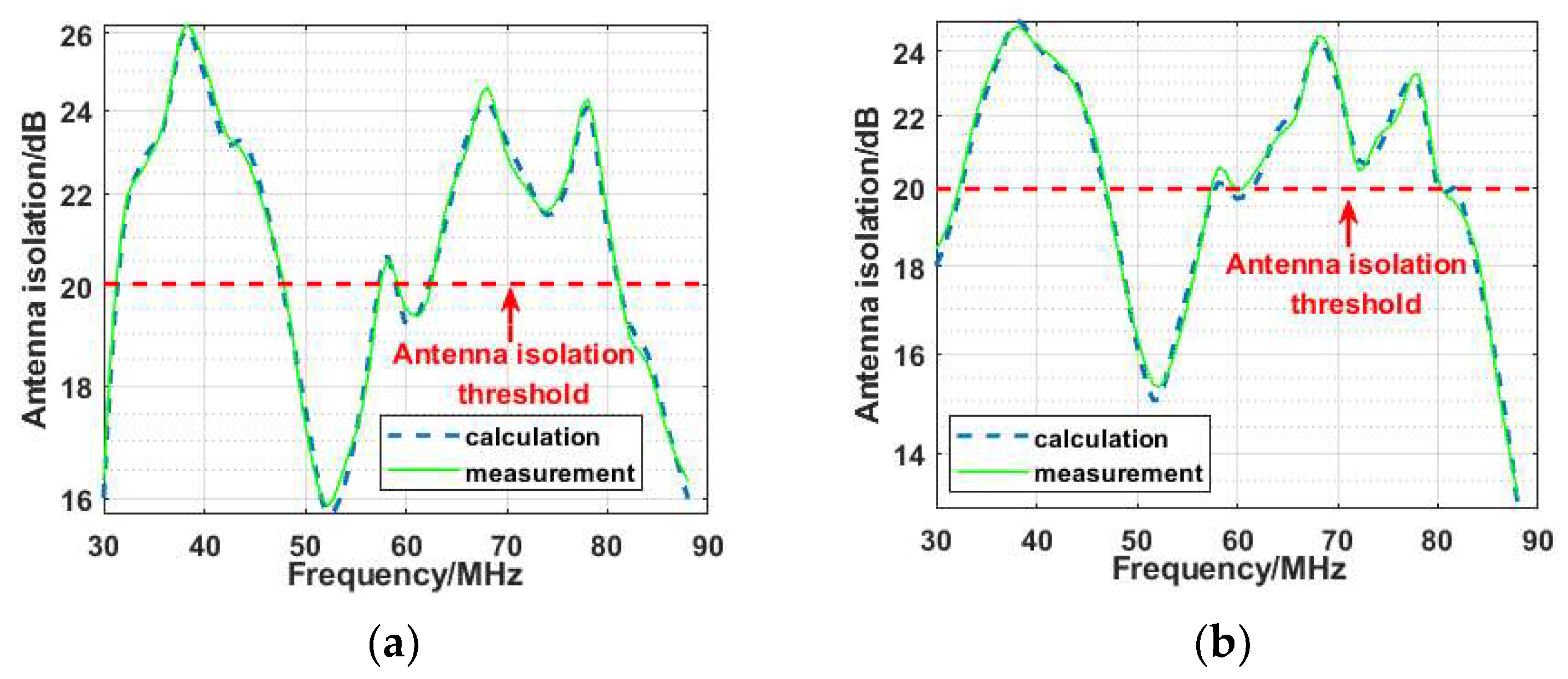
3.4. Level 4 Evaluation: Antenna Isolation

At Level 4, the EMC evaluation focuses on vehicle-mounted antenna isolation. Antenna isolation reflects the degree of influence of electromagnetic signals between antennas [34,35]. The greater the antenna isolation, the smaller the interference. Due to the limited space on the roof of an armored vehicle, the antennas mounted on it are relatively close together. When vehicles communicate, multiple antennas operate simultaneously, and their isolation is reduced. Combined with Equation (12), the antenna isolation is calculated using the following formula:

$$P_{aT}=P_t-L_T+G_t$$

(23)

$$P_{aR}=P_r-L_{\mathrm{R}}+G_r$$

(24)

$$I=10\lg \frac{P_{aT}}{P_{aR}}$$

(25)

Here, $I$ is the antenna isolation, $P_{aT}$ is the actual power of the transmitting antenna, and $P_{aR}$ is the actual power of the receiving antenna.

The above equations can be used to calculate antenna isolation. If the result is less than the threshold of the system EMC, the fourth-level EMC evaluation result will be $\mathrm{IM}>0$, which indicates that a potential EMI is present and a fifth-level evaluation is required.

3.5. Level 5 Evaluation: Communication Performance

The most important function of a vehicular communication system is continuous and effective communication with other vehicles and the C³I system. Therefore, this EMC evaluation focuses on the communication performance of the system, including the calculation and analysis of communication distance and quality.

3.5.1. Communication Distance

The relationship between communication distance and receiver sensitivity decrease is as follows:

$$\frac{d^{\prime }}{d}{=10}^{\frac{-\Delta S}{20}}$$

(26)

Above, $d^{\prime }$ is the communication distance with interference, and $d$ is the communication distance without interference.

The communication distance reduction $\Delta d$ can be given by the following Equation (27).

$$\Delta d=\frac{d-d^{\prime }}{d}(\%)$$

(27)

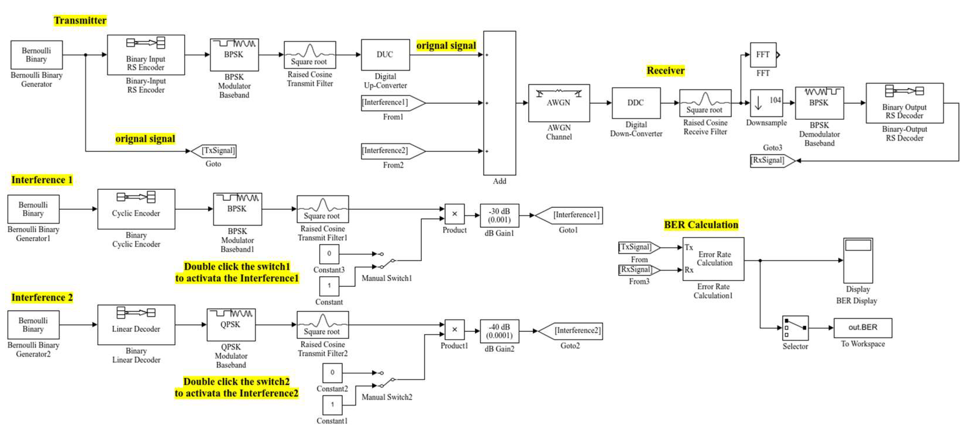
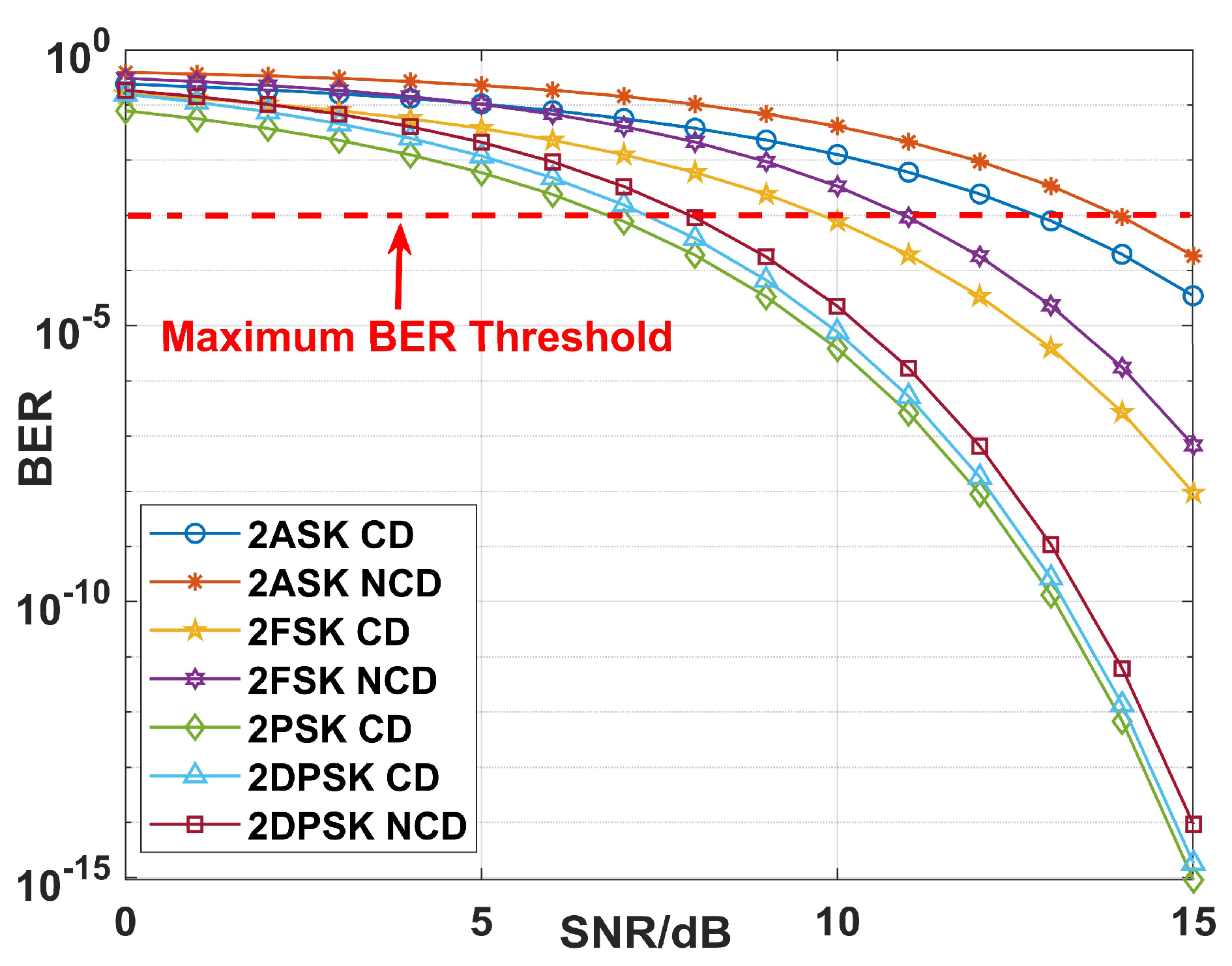
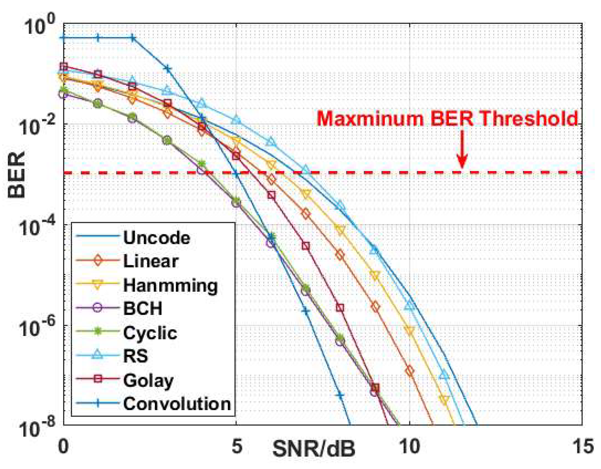
3.5.2. Communication Quality

There are two types of communication systems: digital communication systems and analog communication systems.

(1) Speech articulation

The signal-to-noise ratio (SNR) is the key criterion by which to evaluate the performance of analog communication systems, and it can be calculated using Equation (28). When a radio’s voice communication function is being used, the system performance can be evaluated via speech articulation, which refers to the quality characteristics of human speech sound and can be calculated using Equation (29).

$$SNR=10\lg \frac{S}{N}$$

(28)

$$D=1-\exp \left[-0.06128{\left(SNR+12\right)}^{1.6951}\right]$$

(29)

Here, $D$ is speech articulation, $S$ is signal power, and $N$ is noise power.

(2) Bit Error Rate

In digital communication systems, the bit error rate (BER) is the key criterion used to evaluate the communication performance of a system [36,37]. However, there are many issues that can affect the signal BER, such as the channel-coding mode, the channel environment, or the modulation type. The equations used to calculate the BER for the different modulation types are given in

Table 4. Equations for calculating BER for different modulation types.

Modulation Types	Coherent Modulation	Noncoherent Modulation
2ASK	$\frac{1}{2}erf{c}^1(\frac{\sqrt{SNR}}{2})$	$\frac{1}{2}{e}^{\frac{-SNR}{4}}$
2FSK	$\frac{1}{2}erf{c}^1(\sqrt{\frac{SNR}{2}})$	$\frac{1}{2}{e}^{\frac{-SNR}{2}}$
2PSK	$\frac{1}{2}erf{c}^1(\sqrt{SNR})$	/
2DPSK	$erf{c}^1(\sqrt{SNR})$	$\frac{1}{2}{e}^{-SNR}$

¹ $erfc(x)=\frac{2}{\sqrt{\pi }}{\displaystyle {\int }_x^{\infty }{e}^{-t^2}}dt$.

. The impact of different modulation types and different channel-coding methods on the BER is analyzed in detail in the next section.

4. Application of the Model

In this section, we use the proposed model to perform a system-level EMC evaluation on vehicle 1. Vehicle 2 is the auxiliary vehicle for evaluation. For the provided example, there are two vehicles, and the detailed parameters of the vehicle-mounted radio stations and antennas, as well as system performance indicators, are shown in

Table 5. Vehicle 1 parameters.

No. 1. Shortwave Radio Station (HF1)		No. 2. Ultra-Shortwave Radio Station (VHF2)
Working state	Transmitting	Working state	Transmitting
Working frequency (MHZ)	15	Working frequency (MHZ)	45
Transmission power (W)	50	Transmission power (W)	50
Bandwidth (MHZ)	3	Bandwidth (MHZ)	10
VSWR	1.5	VSWR	1.5
Antenna gain (dB)	1	Antenna gain (dB)	1
Antenna polarization	Vertical polarization	Antenna polarization	Horizontal polarization
No. 3. Ultra-Shortwave Radio Station (VHF3)		Vehicular Performance Indicator
Working state	Receiving	Communication distance (km)	15–30
Working frequency (MHZ)	53	Antenna isolation (dB)	≥20
Sensitivity (dBm)	−116	Decrease in receiver sensitivity (dB)	≤6
Bandwidth (MHZ)	15	Vehicular height (m)	3
VSWR	1.5	Antenna height (m)	2.5
Antenna gain (dB)	1
Antenna polarization	Vertical polarization

and

Table 6. Vehicle 2 parameters.

No. 4. Ultra-Shortwave Radio Station (VHF4)		No. 5. Shortwave Radio Station (HF5)
Working state	Transmitting	Working state	Receiving
Working frequency (MHZ)	80	Working frequency (MHZ)	11
Transmission power (W)	50	Sensitivity (dBm)	−107
Bandwidth (MHZ)	17	Bandwidth (MHZ)	3
VSWR	1.5	VSWR	1.5
Antenna gain (dB)	1	Antenna gain (dB)	1
Antenna polarization	Vertical polarization	Antenna polarization	Vertical polarization
Vehicular Performance Indicator
Vehicular height (m)	3
Antenna height (m)	2.5

.

4.1. Level 1 Evaluation: Work Environment

For the provided example, with the information listed in Table 5 and Table 6, the first-level evaluation can be performed directly based on Equations (5) to (8). The radio stations HF1, VHF2, and VHF3 are selected to make up the two sets of devices to evaluate based on Equations (5) to (8).

From the results of the calculations in

Table 7. Calculation results.

Device Set	FIM	TIM	RIM	SIM
HF1 and VHF3	Absent	Present	Present	Present
VHF2 and VHF3	Present	Present	Present	Present

, we can conclude that TIM, RIM, and SIM are present between HF1 and VHF3. Similarly, FIM, TIM, RIM, and SIM are present between VHF2 and VHF3. The first-level evaluation result is $\mathrm{IM}>0$, which indicates that a potential EMI is present in this system and a second-level evaluation is required.

4.2. Level 2 Evaluation: Signal Spectrum

In the second-level evaluation, with the information listed in Table 5 and Table 6, the system can directly predict the possible types of spectral interference between the transmitter and the receiver. The radio stations HF1, VHF3 and VHF2, and VHF3 are selected to make up the two sets of devices for evaluating fundamental wave interference based on Equation (9). The radio stations HF1, VHF3 and VHF2, and VHF3 are selected to make up the two sets of devices for evaluating harmonic wave interference based on Equation (10). Based on the frequencies of the transmitter and receiver, we must choose an appropriate value of n to calculate. We then increment the order coefficient n and repeat the calculation until all orders of interest have been analyzed for both sets of devices. The radio stations HF1, VHF2, and VHF3 make up the set of devices for evaluating the intermediation wave interference based on Equation (11). Based on the frequencies of the transmitter and receiver, we chose the appropriate n and m for the calculation. We then incremented the order coefficients m and n and repeated the calculation until all orders of interest had been analyzed.

From the synthesis of all the calculations in

Table 8. Calculation results.

Device Set	Fundamental Wave Interference	High-Order Harmonic Wave Interference	High-Order Intermediation Interference
HF1 and VHF3	Absent	Present	/
VHF2 and VHF3	Present	Absent	/
HF1,VHF2 and VHF3	/	/	Present

, we conclude that there is potential fundamental wave interference for VHF2 and VHF3, potential higher-order harmonic interference for HF1 and VHF3, and potential higher-order intermediate interference for HF1, VHF2, and VHF3. Hence, the second-level evaluation result is $\mathrm{IM}>0$, which indicates that some potential EMI is present in the system and that the evaluation should proceed to the next level.

4.3. Level 3 Evaluation: Sensitivity of the Receiver

The reduction in the VHF3 receiver sensitivity in vehicle 1 when it communicates with the VHF4 transmitter in vehicle 2 is evaluated at this level. According to the information listed in Table 5; Table 6, it can be seen that the polarization mismatch loss corresponds to $L_{\mathrm{C}}=0$ and the feed losses correspond to $L_{\mathrm{T}}=0.51$ and $L_{\mathrm{R}}=0.51$.

Using remote sensing technology, a satellite map of the area between the two vehicles could be obtained; this is shown in Figure 3. Based on the digital map, a contour map and a topographic profile of the actual communication path between the two vehicles could be obtained; these are shown in Figure 4 and Figure 5. The model diagram of the actual communication path between the two vehicles is shown in Figure 6. The actual communication distance can be given by the following Equation (26).

$$d=\sqrt{{\left[\left(h_{ar}+H_{\mathrm{v}1}+H_1\right)-\left(h_{at}+H_{\mathrm{v}2}+H_2\right)\right]}^2+D_t{}^2}$$

(30)

Here, $H_{\mathrm{v}1}$ is the height of vehicle 1, $h_{ar}$ is the receiving antenna’s height, $H_1$ is the altitude at which vehicle 1 is located, $H_{\mathrm{v}2}$ is the height of vehicle 2, $h_{at}$ is the transmitting antenna height, $H_2$ is the altitude at which vehicle 2 is located, and $D_t$ is the topographic distance.

The radio wave propagation loss in free space was calculated between two vehicles using Equation (12). The Egli model was used to calculate the propagation loss of the two vehicles using Equation (13). Based on the topographic profile, the propagation loss between the two vehicles on real terrain was calculated using Equations (12) and (30); the results are shown in Figure 7.

The actual power received by receiver VHF3 was measured at different topographic distances, as shown in

Table 9. Actual received power at different terrain distances.

D (km)	15	16	17	18	19	20	21	22
Actual received power (dBm)	−123.6	−124.3	−125.1	−125.5	−126.1	−126.8	−127.2	−127.8
D (km)	23	24	25	26	27	28	29	30
Actual received power (dBm)	−128.4	−129.1	−130.2	−130.8	−131.4	−131.8	−132.6	−133.1

.

The received power of the receiver was calculated according to the free-space propagation loss and the actual terrain propagation loss, and the received power was compared with the actual measurements, as shown in Figure 8.

Figure 8 shows that the error between the calculated power received by the receiver in free space and the real measurement is 3.03%. The error of the calculated power received by the receiver in the actual terrain and the real measurement is 2.06%. The error was reduced by 0.97%. When the communication distance is greater than 20 km, there are large errors, and there are even errors when the Egli model is used to calculate the propagation loss and the received power at the receiver. This is because the Egli model is not suitable for communication regions with large terrain fluctuations. Therefore, no comparison with the Egli model is given in Figure 9.

According to the received power of the receiver in free space, on actual terrain, and in the actual measurement data, the sensitivity reduction of the receiver in three cases was calculated using Equation (18), as shown in Figure 9.

As can be seen in Figure 9, the broken red line indicates the receiver sensitivity reduction threshold. Depending on the threshold of the EMC indicators of the system, the sensitivity reduction of the radio receiver should be less than 6 dB. The sensitivity of the receiver is reduced by more than 6 dB when the communication distance exceeds 15.5 km in real measurements. The sensitivity of the receiver is reduced by more than 6 dB when the communication distance exceeds 16.5 km on the actual terrain. The sensitivity of the receiver is reduced by more than 6 dB when the communication distance exceeds 19.1 km in free space. The error in the calculation of the receiver sensitivity reduction in free space and via measurement is 23.23%. The error in the calculation of the receiver sensitivity reduction in the actual terrain and via measurement is 6.45%. Thus, the error was reduced by 16.78%.

Therefore, the evaluation result is $\mathrm{IM}>0$, which indicates that a potential EMI is present and a fourth-level evaluation is required.

4.4. Level 4 Evaluation: Antenna isolation

At this level, the isolation of the vehicle-mounted antennas was evaluated. The isolation degree between the receiving antenna connected to the VHF3 receiver and the transmitting antenna connected to the HF1 and VHF2 transmitters was calculated, and the results obtained via calculation and measurement are shown in Figure 10.

As shown in Figure 10a, the calculation of the level of antenna isolation between HF1 and VHF3 is in good agreement with the measurement, and it is less than 20 dB in the ranges of 48 MHz to 57 MHz and 81 MHz to 88 MHz. Figure 10b shows that the calculated antenna isolation between VHF2 and VHF3 is in good agreement with the measurement, and it is less than 20 dB in the ranges of 47 MHz to 58 MHz and 80 MHz to 88 MHz. The broken red line in Figure 6 represents the antenna isolation threshold. Depending on the system EMC threshold, the level of antenna isolation usually must be greater than 20 dB. Therefore, the evaluation result of this level is $\mathrm{IM}>0$, which indicates that a potential EMI is present in this system and fifth-level evaluation is required.

4.5. Level 5 Evaluation: Communication Performance

As mentioned above, the most crucial function of an armored vehicle communication system is to maintain effective and continuous communication with other vehicles and the C³I system. Consequently, the fifth-level evaluation focuses on communication performance.

4.5.1. Communication Distance

For the provided example, we first computed the communication distance of the armored vehicle in free space and on actual terrain and compared it with the communication distance in the absence of interference to determine the reduction in the communication distance, which are shown in Figure 11.

4.5.2. Communication Quality

In the application example, the communication system is a digital communication system, and the communication signal is an audio signal. Therefore, the fifth-level evaluation is based on the BER, and the IM criterion is defined based on the maximum acceptable BER. As we can see in

Table 10. BER thresholds for different types of digital signals.

Signal Type	BER Threshold
Audio Signals	$P_{\mathrm{e}}\le 1\times {10}^{-3}$
Image Signals	$P_{\mathrm{e}}\le 1\times {10}^{-5}$
Video Signals	$P_{\mathrm{e}}\le 1\times {10}^{-9}$

, the maximum BER threshold for audio signals is $P_{\mathrm{e}}=1\times {10}^{-3}$. Therefore, $P_{\mathrm{e}}=1\times {10}^{-3}$ was identified as the fifth-level IM criterion.

In practice, there are various factors that affect the BER, such as the modulation mode and the channel-coding mode. Hence, these two factors are discussed in this paper. To compute the BER of the audio signal in the proposed example, we selected some channel-coding modes and modulation modes commonly used in armored vehicle communication systems and constructed a simplified simulation model of a typical communication link, which is shown in Figure 12.

(1) The influence of the modulation type

Figure 13 shows the relationship between BER and SNR for seven modulation types: 2PSK coherent modulation, 2DPSK coherent modulation, 2DPSK incoherent modulation, 2FSK coherent modulation, 2FSK incoherent modulation, 2ASK coherent modulation, and 2ASK incoherent modulation. The broken red line in Figure 12 represents the maximum BER threshold for distinguishable audio signals.

As shown in Figure 13, the degrees of electromagnetic compatibility of the seven modulation modes of the armored vehicle’s digital communication system are ranked from highest to the lowest: 2PSK coherent modulation, 2DPSK coherent modulation, 2DPSK incoherent modulation, 2FSK coherent modulation, 2FSK incoherent modulation, 2ASK coherent modulation, and 2ASK incoherent modulation. From the point of view of systematic EMC evaluation, it can be argued that 2PSK coherent modulation has the best EMC.

(2) The influence on the channel-coding mode

Figure 14 shows the relationship between BER and SNR for seven channel-coding modes: convolutional coding, BCH coding, cyclic coding, Golay coding, linear coding, Hamming coding, and RS coding. The broken red line in Figure 13 represents the maximum BER threshold for distinguishable audio signals.

As shown in Figure 14, the levels of electromagnetic compatibility of the seven channel-coding modes of the armored vehicle digital communication system are ranked from the highest to the lowest: convolutional coding, BCH coding, cyclic coding, Golay coding, linear coding, Hamming coding, and RS coding. From the point of view of systematic EMC evaluation, it can be argued that convolution coding has the best EMC.

Based on the BER simulation results, the evaluation result of this level is $\mathrm{IM}>0$, which indicates that a potential EMI is present in this system.

In summary, all evaluation processes have been completed. There is a potential for EMI and a possible risk of electromagnetic incompatibility in the communications system of the armored vehicle according to our review of the evaluation results.

5. Discussion

In Section 3, the architecture of the proposed model was outlined, and the evaluation methods applied on each level were explored. An example of the proposed model was presented in Section 4. In this section, the performance of the proposed model is discussed.

(1) The proposed model can quickly evaluate whether any of four kinds of interference margins are present between transmitters and receivers.

(2) The proposed model can quickly evaluate whether any of three kinds of signal spectrum interference are present between transmitters and receivers.

(3) The decrease in receiver sensitivity is one of the important factors affecting vehicle communication and one of the important indicators of vehicle electromagnetic compatibility. The traditional model does not evaluate the change in receiver sensitivity. The proposed model obtains the terrain profile through a digital map and obtains the actual distance of vehicle communication. Considering feed loss, antenna polarization mismatch loss, and propagation loss, the actual power and sensitivity decline of the receiver were calculated. The sensitivity of the receiver was evaluated through comparison with the vehicle EMC indicators.

(4) The signal transmission of the communication system is based on vehicle-mounted antennas. Due to the various types and numbers of antennas mounted on the vehicle, antenna isolation will be reduced, and the quality of signal transmission will be affected. However, traditional models do not evaluate the degree of isolation between antennas. The proposed model can be used to calculate the decreasing degree of isolation of the vehicle-mounted antenna and evaluate it by comparing it with the vehicular communication system EMC indicators.

(5) In the past, most types of communication systems were analog systems, for which traditional models are suitable. However, with the development of electronic science and technology, most communication systems are now digital, and traditional evaluation models are less efficient. The proposed model is suitable not only for evaluating analog systems but also digital systems. If analog and digital systems are used for voice communication, they can be evaluated using speech clarity and BER, respectively.

(6) The most important function of an armored vehicular communication system is the ability to effectively and continuously communicate with other vehicles and C³I systems. Various communication systems have different requirements for communication distance under different conditions. Traditional models cannot be used to evaluate changes in communication distance. The degree of decrease in communication distance can be determined using the proposed model.

(7) In this article, a link simulation model was established based on an actual communication system, and the influence of the modulation mode and coding mode on the bit error rate of the analyzed armored vehicle digital communication system was analyzed. The modulation mode and coding mode with the best electromagnetic compatibility were determined. The proposed model can evaluate BER by comparing it with vehicular communication system EMC indicators.

In summary, each evaluation model has its advantages and disadvantages. The evaluation model proposed in this paper is especially suitable for armored vehicle communication systems.

6. Conclusions

In this research, the performance of armored vehicle communication systems was studied systematically, and a five-level evaluation model was proposed from the perspective of system electromagnetic compatibility. This model can evaluate the electromagnetic compatibility of a vehicular communication system in relation to five aspects: working environment, signal spectrum, antenna isolation, receiver sensitivity, and communication performance. Finally, the proposed evaluation model was verified through an example armored vehicle, and great results were obtained, proving the applicability of the five-level evaluation model. In particular, when the receiver sensitivity was evaluated in the third level, a more accurate vehicle communication propagation model was established based on the digital maps. The model can determine the terrain profile on the vehicle communication path and the actual communication distance. The actual power received by the receiver and the sensitivity reduction of the receiver on real terrain can be calculated. Compared with the free-space propagation model, the error of the actual power received by the receiver was reduced by 0.97%, and the error of the communication distance for which the sensitivity of the receiver was reduced by more than the system EMC threshold was reduced by 16.78%. In the fourth- and fifth-level evaluations, some of the calculation results from the third-level evaluation were also applied. The calculated antenna isolation degrees were basically consistent with the actual measurement data, and a more accurate communication distance decline was obtained. In summary, the evaluation model based on digital maps proposed in this paper is more accurate than previous models. The development of remote sensing technology and the application of digital maps are helpful for constructing an accurate system-level EMC evaluation model, which can also be beneficial in guiding future efforts regarding the EMC design of armored communication systems and reducing design cycles.

References

1. Aiello, O.; Crovetti, P. Characterization of the Susceptibility to EMI of a BMS IC for Electric Vehicles by Direct Power and Bulk Current Injection. IEEE Lett. Electromagn. Compat. Pract. Appl. 2021, 3, 101–107. [Google Scholar] [CrossRef]
2. Wang, K.; Lu, H.; Chen, C.; Xiong, Y. Modeling of System-Level Conducted EMI of the High-Voltage Electric Drive System in Electric Vehicles. IEEE Trans. Electromagn. Compat. 2022, 64, 741–749. [Google Scholar] [CrossRef]
3. Wang, K.; Lu, H.; Li, X. High-Frequency Modeling of the High-Voltage Electric Drive System for Conducted EMI Simulation in Electric Vehicles. IEEE Trans. Transp. Electrif. 2023, 9, 2808–2819. [Google Scholar] [CrossRef]
4. Gajbhiye, P.; Achari, K.N.; Balakrishna, G.; Kumar, M.V. An Approach to Mitigate the EMI Noise Effect in Vehicle-to-Grid (V2G) System. In Proceedings of the 2021 2nd Global Conference for Advancement in Technology (GCAT), Bangalore, India, 1–3 October 2021; pp. 1–6. [Google Scholar]
5. Qian, W.; Yang, Y.; Peng, J.; Cao, H.; Li, X.; Gao, Y.; Lei, J. EMI Modeling for Vehicle Body using Characteristic Mode Analysis. In Proceedings of the 2022 Asia-Pacific International Symposium on Electromagnetic Compatibility (APEMC), Beijing, China, 1–4 September 2022; pp. 732–734. [Google Scholar]
6. Qian, W.; Yang, Y.; Peng, J.; Cao, H.; Li, X.; Gao, Y.; Lei, J. Vehicle electromagnetic interference suppression using characteristic mode analysis. In Proceedings of the 2022 Asia-Pacific International Symposium on Electromagnetic Compatibility (APEMC), Beijing, China, 1–4 September 2022; pp. 427–429. [Google Scholar]
7. Mutoh, N.; Nakanishi, M.; Kanesaki, M.; Nakashima, J. EMI noise control methods suitable for electric vehicle drive systems. IEEE Trans. Electromagn. Compat. 2005, 47, 930–937. [Google Scholar] [CrossRef]
8. Pliakostathis, K. Research on EMI from Modern Electric Vehicles and their Recharging Systems. In Proceedings of the 2020 International Symposium on Electromagnetic Compatibility-EMC EUROPE, Rome, Italy, 23–25 September 2020; pp. 1–6. [Google Scholar]
9. Jiang, L.; Liu, H.; Zhang, X. Analysis on EMC influencing factors of electric vehicle wireless charging system. In Proceedings of the 2021 IEEE International Joint EMC/SI/PI and EMC Europe Symposium, Raleigh, NC, USA, 26 July–13 August 2021; pp. 285–290. [Google Scholar]
10. Alcaras, A. EMC Performances of a Land Army Vehicle to Respect Integrated Radios Reception Sensitivity: Typical Performances Needed for “Fitted for Radio (FFR)” Land Vehicle. In Proceedings of the 2018 International Symposium on Electromagnetic Compatibility (EMC EUROPE), Amsterdam, The Netherlands, 27–30 August 2018; pp. 303–308. [Google Scholar]
11. Gkatsi, V.; Vogt-Ardatjew, R.; Leferink, F. Risk-based EMC System Analysis Platform of Automotive Environments. In Proceedings of the 2021 IEEE International Joint EMC/SI/PI and EMC Europe Symposium, Raleigh, NC, USA, 26 July–13 August 2021; pp. 749–754. [Google Scholar]
12. Zhao, T.; Liu, X.; Sun, P.; An, M.; Mu, X. EMC Vehicle-Level Layout Design for Railway Vehicles in Complex Electromagnetic Environment. In Proceedings of the 2021 11th International Conference on Information Technology in Medicine and Education (ITME), Wuyishan, China, 19–21 November 2021; pp. 231–236. [Google Scholar]
13. Hein, J.; Hippeli, J.; Eibert, T.F. Efficient EMC Parameter Analysis for the Verification of Complex Automotive Simulation Models by the Utilization of Design of Experiments. IEEE Trans. Electromagn. Compat. 2018, 60, 1965–1973. [Google Scholar] [CrossRef]
14. Isaacs, J.; Mcnair, T.; Momson, R. A program for analyzing co-site interferences. In Proceedings of the 1992 International Conference on Tactical Communications, Fort Wayne, IN, USA, 28–30 April 1992; pp. 119–124. [Google Scholar]
15. Chen, H.; Wang, G. Research of frequency assignment based on genetic algorithm. In Proceedings of the 2009 3rd IEEE International Symposium on Microwave, Antenna, Propagation and EMC Technologies for Wireless Communications, Beijing, China, 27–29 October 2009; pp. 199–202. [Google Scholar]
16. Baldwin, T.E.; Capraro, G.T. Intrasystem electromagnetic compatibility program (IEMCAP). IEEE Trans. Electromagn. Compat. 1980, 22, 224–228. [Google Scholar] [CrossRef]
17. Duff, W.G.; Foster, J.J. Nonlinear effects models for the intrasystem electromagnetic compatibility analysis program (IEMCAP). In Proceedings of the 1981 IEEE International Symposium on Electromagnetic Compatibility, Boulder, CO, USA, 18–20 August 1981; pp. 238–245. [Google Scholar]
18. Hilbert, A.L. An overview of the air force intrasystem analysis program (IAP). In Proceedings of the 1975 IEEE International Symposium on Electromagnetic Compatibility, San Antonio, TX, USA, 7–9 October 1975; pp. 1–3. [Google Scholar]
19. Zhou, P.; Lv, Y.; Chen, Z.; Xu, H. System-level EMC assessment for military vehicular communication systems based on a modified four-level assessment model. China Commun. 2018, 15, 39–53. [Google Scholar] [CrossRef]
20. Violette, N.J.L.; Write, R.J.; Violette, M.F. Electromagnetic Compatibility Handbook; Van Norstrand Reinhold Company Inc.: New York, NY, USA, 1987. [Google Scholar]
21. Wang, C.; Wen, C.; Cheng, M.; Liu, M.Z.; Li, X. LiDAR-based localization using universal encoding and memory-aware regression. Pattern Recognit. 2022, 128, 108685. [Google Scholar]
22. Yu, S.; Wang, C.; Lin, Y.; Wen, C.; Cheng, M.; Hu, G. STCLoc: Deep LiDAR Localization With Spatio-Temporal Constraints. IEEE Trans. Intell. Transp. Syst. 2023, 24, 489–500. [Google Scholar] [CrossRef]
23. Yu, S.; Wang, C.; Yu, Z.; Li, X.; Cheng, M.; Zang, Y. Deep regression for LiDAR-based localization in dense urban areas. ISPRS J. Photogramm. Remote Sens. 2021, 172, 240–252. [Google Scholar] [CrossRef]
24. Li, W.; Yu, S.; Wang, C.; Hu, G.; Shen, S.; Wen, C. SGLoc: Scene Geometry Encoding for Outdoor LiDAR Localization. In Proceedings of the 2023 IEEE/CVF Conference on Computer Vision and Pattern Recognition (CVPR), Vancouver, BC, Canada, 17–24 June 2023. [Google Scholar]
25. Li, H.; He, W.; He, X. Prediction of Radio Wave Propagation Loss in Ultra-Rugged Terrain Areas. IEEE Trans. Antennas Propag. 2021, 69, 4768–4780. [Google Scholar] [CrossRef]
26. Kvicera, M.; Pechac, P.; Valtr, P. Influence of Input Terrain Profile Resolution on Diffraction Modeling. IEEE Antennas Wirel. Propag. Lett. 2014, 14, 1318–1321. [Google Scholar] [CrossRef]
27. Sunarya, I.M.G.; Al Affan, M.R.; Kurniawan, A.; Yuniarno, E.M. Digital Map Based on Unmanned Aerial Vehicle. In Proceedings of the 2020 International Conference on Computer Engineering, Network, and Intelligent Multimedia (CENIM), Surabaya, Indonesia, 17–18 November 2020; pp. 211–216. [Google Scholar]
28. Zhu, Q.; Jiang, S.; Wang, C.-X.; Hua, B.; Mao, K.; Chen, X.; Zhong, W. Effects of Digital Map on the RT-based Channel Model for UAV mmWave Communications. In Proceedings of the 2020 International Wireless Communications and Mobile Computing (IWCMC), Limassol, Cyprus, 15–19 June 2020; pp. 1648–1653. [Google Scholar]
29. Genender, E.; Garbe, H.; Sabath, F. Probabilistic risk analysis technique of intentional electromagnetic interference at system level. IEEE Trans. Electromagn. Compat. 2014, 56, 200–207. [Google Scholar] [CrossRef]
30. Agili, S.S.; Ishii, T.K. Electromagnetic compatibility of PSK-OOK digital fiber communications. IEEE Trans. Electromagn. Compat. 2014, 56, 1322–1325. [Google Scholar] [CrossRef]
31. Manzi, G.; Feliziani, M.; Beeckman, P.A.; van Dijk, N. Coexistence between ultra-wideband radio and narrow-band wireless LAN communication systems-part II: EMI evaluation. IEEE Trans. Electromagn. Compat. 2009, 51, 382–390. [Google Scholar] [CrossRef]
32. Songbai, H.; Mingyu, L.; Hongmin, D.; Juebang, Y. Analysis of CDMA RF channel nonlinear distortion. In Proceedings of the International Conference on Communication Circuits and Systems, Chengdu, China, 29 June–1 July 2002; pp. 474–477. [Google Scholar]
33. Tait, G.B.; Richardson, R.E.; Slocum, M.B.; Hatfield, M.O. Time-Dependent Model of RF energy propagation in coupled reverberant cavities. IEEE Trans. Electromagn. Compat. 2011, 53, 846–849. [Google Scholar] [CrossRef]
34. Malmstrom, J.; Frid, H.; Jonsson, B.L.G. Approximate methods to determine the isolation between antennas on vehicles. In Proceedings of the 2016 IEEE International Symposium on Antennas and Propagation (APSURSI), Fajardo, PR, USA, 26 June–1 July 2016; pp. 131–132. [Google Scholar]
35. Kolodziej, K.E.; Perry, B.T. Vehicle-mounted STAR antenna isolation performance. In Proceedings of the 2015 IEEE International Symposium on Antennas and Propagation & USNC/URSI National Radio Science Meeting, Vancouver, BC, Canada, 19–24 July 2015; pp. 1602–1603. [Google Scholar]
36. Popovici, A.C. Fast measurement of bit error rate and error probability estimation in digital communication systems. In Proceedings of the IEEE GLOBECOM, Sydney, NSW, Australia, 8–12 November 1998; Volume 5, pp. 2736–2739. [Google Scholar]
37. Hsiao, H.-F.; Lin, S.-G.; Su, S.-H.; Tu, C.H.; Chang, D.C.; Juang, Y.Z.; Chiou, H.K. Bit error rate measurement system for RF integrated circuits. In Proceedings of the 2012 IEEE International Instrumentation and Measurement Technology Conference Proceedings, Graz, Austria, 13–16 May 2012; pp. 2381–2384. [Google Scholar]
Figure 1. Flowchart of the proposed evaluation model.
Remotesensing 15 04872 g001
Figure 2. Vehicle-communication-propagation-model-based graphical depiction of terms used in the transmission loss.
Remotesensing 15 04872 g002
Figure 3. Satellite map of the area between the two vehicles.
Remotesensing 15 04872 g003
Figure 4. Contour map of the actual communication path.
Remotesensing 15 04872 g004
Figure 5. Topographic profile of the actual communication path.
Remotesensing 15 04872 g005
Figure 6. Model diagram of the actual communication path.
Remotesensing 15 04872 g006
Figure 7. Comparison of propagation loss under three conditions.
Remotesensing 15 04872 g007
Figure 8. Actual power received by receiver VHF3.
Remotesensing 15 04872 g008
Figure 9. Sensitivity reduction of receiver VHF3.
Remotesensing 15 04872 g009
Figure 10. Comparison of the results from the calculation and measurement of antenna isolation. (a) HF1 and VHF3; (b) VHF2 and VHF3.
Remotesensing 15 04872 g010
Figure 11. Relationship between the receiver VHF3 sensitivity reduction and the communication distance reduction.
Remotesensing 15 04872 g011
Figure 12. Simulation model of the communication link.
Remotesensing 15 04872 g012
Figure 13. Relationship between BER and SNR for seven modulation types.
Remotesensing 15 04872 g013
Figure 14. Relationship between BER and SNR for seven channel-coding modes.
Remotesensing 15 04872 g014