Revealing the Potential of Deep Learning for Detecting Submarine Pipelines in Side-Scan Sonar Images: An Investigation of Pre-Training Datasets

Abstract

This study introduces a novel approach to the critical task of submarine pipeline or cable (POC) detection by employing GoogleNet for the automatic recognition of side-scan sonar (SSS) images. The traditional interpretation methods, heavily reliant on human interpretation, are replaced with a more reliable deep-learning-based methodology. We explored the enhancement of model accuracy via transfer learning and scrutinized the influence of three distinct pre-training datasets on the model’s performance. The results indicate that GoogleNet facilitated effective identification, with accuracy and precision rates exceeding 90%. Furthermore, pre-training with the ImageNet dataset increased prediction accuracy by about 10% compared to the model without pre-training. The model’s prediction ability was best promoted by pre-training datasets in the following order: Marine-PULSE ≥ ImageNet > SeabedObjects-KLSG. Our study shows that pre-training dataset categories, dataset volume, and data consistency with predicted data are crucial factors affecting pre-training outcomes. These findings set the stage for future research on automatic pipeline detection using deep learning techniques and emphasize the significance of suitable pre-training dataset selection for CNN models.

1. Introduction

Submarine pipelines and cables provide the primary transportation and energy support for the development of offshore oil and gas resources. Given their critical role, their health and integrity are paramount for both economic and ecological well-being. Their leakage, often due to suspension or deformation, can lead to substantial economic and ecological damage, highlighting the importance of detecting subsea pipelines. Extracting valuable information from underwater environments is crucial for oceanographic studies and maritime applications, with pipeline or cable (POC) detection emerging as a critical task for safety and operational reasons [1,2]. Traditionally, this task has largely relied on side-scan sonar (SSS) imaging, which provides high-resolution imagery of the seafloor. However, this method necessitates intensive manual interpretation, which is time-consuming and prone to human error [3,4], emphasizing the need for a more automated and efficient process.

In recent years, artificial intelligence methods have made significant strides in geological fields, including remote sensing [5,6,7,8], geological hazard prediction [9,10,11,12,13,14,15,16], geological exploration [17,18,19,20,21,22], and energy development [23]. However, the applicability and effectiveness of these methods in the specialized field of pipeline or cable (POC) detection remain inadequately explored. This represents a significant gap given the critical nature of POC detection in safeguarding both environmental and industrial interests. Convolutional neural networks (CNNs), in particular, have shown promise in the field of underwater data processing. This provides an opportunity to employ CNNs in tackling the intricate task of POC detection, which is crucial for both environmental protection and industrial operations. Initial applications of CNNs to underwater data were primarily in areas such as fish species identification and sea-floor mapping [1,24]. While these areas are important, they are notably less complex in terms of the variety and nuances of the data involved compared to POC detection. With advancements in technology, researchers began applying CNNs to more complex tasks, such as underwater wreck detection [25,26], the real-time processing of side-scan sonar data [27], and developing novel models for SSS image recognition such as U-Net [28] and VIT [29]. The focus of our work was to address the limited availability and quality of training data, a problem that was not adequately addressed in previous studies. Moreover, we aimed to investigate the role of different pre-training datasets in enhancing the predictive accuracy of CNN models specifically for POC detection. This transition was driven by a combination of the increasing complexity and volume of underwater data and the enhancement in the computational power of machine learning systems. Consequently, studies began investigating various deep learning networks’ predictive abilities, focusing on their applicability and effectiveness for SSS image prediction [30]. Still, one glaring gap remained: the scarcity and quality of data available for training these deep learning models.

While deep learning has achieved commendable results in predicting side-scan sonar images, the challenge of acquiring this type of data and the limited availability of existing datasets remain pressing issues. Common research methodologies typically involve analyzing a range of algorithms against a single public dataset (such as SeabedObjects-KLSG [31]). Although these advances hint at the potential use of CNNs in POC detection, they do not fully address the key challenges of the dataset. Most studies are constrained by the limited availability and quality of training datasets. On one hand, there is a challenge in obtaining sufficient datasets due to the difficulty in acquiring marine data. On the other hand, the datasets are not broad enough, making it difficult to apply them to other regions, even if high accuracy is achieved on a single dataset. Thus, understanding how to efficiently use transfer learning to obtain the best prediction based on limited data is important. This provides room for potential improvements in model prediction accuracy and expands the scope of future research in this area. Therefore, investigating the influence of different pre-training datasets on modeling and proposing how to better utilize the existing datasets to enhance the predictive accuracy of CNN models is of vital importance.

The primary objective of this study was to address these gaps and challenges. Specifically, we planned to use seafloor SSS images from the Yellow River Estuary in China. We aimed to employ the GoogleNet model to investigate three areas: the model’s feasibility for undersea pipeline recognition, the effect of transfer learning on pipeline recognition accuracy, and the influence of different pre-training datasets on pipeline recognition accuracy. By doing so, we made the following contributions: (1) we employed GoogleNet to automate the POC detection process, aiming to surpass the limitations associated with human interpretation; (2) we assessed and analyzed the benefits of transfer learning and its impact on improving POC recognition accuracy; and (3) we comprehensively evaluated the influence of different pre-training datasets on the predictive accuracy of CNN models in the context of POC detection.

Our study aims to contribute to the growing field of automated POC detection using deep learning techniques. In doing so, we not only advance the technological capabilities of POC detection but also provide vital insights for dataset selection and transfer learning, a crucial yet often overlooked aspect of the implementation of CNN models. These insights will undoubtedly serve as a cornerstone for future research endeavors.

2. Applied CNN Model

2.1. GoogleNet

GoogleNet, pioneered by Christian Szegedy [32] at Google, heralded a new era for deep neural networks with the introduction of the innovative Inception architecture. Notably, in the ILSVRC 2014 competition, GoogleNet was used to set a new record in large-scale image recognition tasks, leveraging the ImageNet dataset. This dataset, which contains over a million images spanning 1000 categories, has become a standard for evaluating the capabilities of various deep learning models. GoogleNet’s performance in the ImageNet challenge was particularly compelling, achieving a top-5 error rate of only 6.67%, thereby outperforming many contemporary architectures. Unlike its preceding sequential CNN networks, the Inception structure incorporated internal parallel connections, enabling data to traverse four simultaneous paths, each using different convolutional kernels. As depicted in Figure 1, this design extracts features at multiple scales, enhancing accuracy in the final classification stage when the aggregated results merge into a new network layer.

The advent of GoogleNet’s Inception structure signified a considerable shift from traditional CNN networks, offering two main advantages. First, the concurrent convolution at multiple scales facilitates feature extraction at different abstraction levels, providing a more holistic and nuanced comprehension of the input data. This results in enhanced accuracy and more reliable classification decisions. Second, GoogleNet incorporates 1 × 1 convolutions for dimensionality reduction, considerably minimizing computational complexity. By reducing the number of features prior to further convolutions, it alleviates the computational load, yielding faster, more efficient processing.

The remarkable reduction in computational complexity achieved through GoogleNet’s Inception architecture signifies a significant breakthrough in deep learning. By leveraging dimensionality reduction techniques, such as 1 × 1 convolutions, the network successfully balances computational efficiency with accuracy. This allows the creation of deeper, more potent neural networks capable of handling intricate tasks without overburdening computational resources.

Focusing on the automatic recognition of side-scan sonar images of underwater objects, Du et al. [30] utilized AlexNet, VGG16, GoogleNet, and ResNet to train on and predict the same dataset. While assessing these models, they emphasized prediction precision and computational economy. Their findings underscored GoogleNet’s exemplary prowess in both domains. What resonated with our research goals was GoogleNet’s balance of computational efficiency and model depth. Unlike AlexNet, which might be simpler but is less accurate for intricate datasets, or VGG16, which can be computationally intensive, GoogleNet provided the perfect middle ground. Consequently, we selected GoogleNet to study submarine pipeline recognition using SSS images in this research.

2.2. Transfer Learning

Transfer learning represents a system’s capability to apply knowledge and skills acquired from earlier tasks to new, different tasks. This concept was first introduced by Google Inc. [33] at the 2016 NIPS conference and revolutionized the field of machine learning. Essentially, transfer learning repurposes a previously trained model for a similar problem, achieving better performance than a model trained from scratch. This process mirrors human learning, where proficiency in one skill enhances the learning of similar skills.

The procedure for training a convolutional neural network (CNN) can benefit significantly from transfer learning. Instead of initiating training from scratch, one can employ a pre-training classical model as a foundation and fine-tune its structure and data for retraining. This strategy yields superior results due to the valuable general features and representations the base model has already learned, which are often applicable across diverse domains or tasks. By leveraging this existing knowledge and adjusting it to the specific problem, transfer learning facilitates faster convergence, improved accuracy, and enhanced generalization.

A significant advantage of transfer learning lies in its ability to address the challenge of insufficient training data. In real-world scenarios, amassing a large and diverse dataset for training a model from scratch can be a daunting, resource-intensive task. However, using pre-training models, typically trained on extensive datasets, allows us to transfer the learned patterns and rich feature representations from the source domain to the target domain. This approach enables a model to leverage this knowledge, even when confronted with limited data in the target domain, leading to effective and efficient learning.

Many studies, including studies of remote sensing image classification [34], SAR image classification [35], high-resolution satellite image recognition [36], etc., have compared the improvement in accuracy before and after using transfer learning. However, a more detailed study of how different pre-training datasets affect the final performance of a model has not been conducted. In this paper, we will discuss the impact of pre-training (based on the ImageNet dataset) on model accuracy and the impact of pre-training on model accuracy for different datasets (ImageNet, SeabedObjects-KLSG, and Marine-PULSE). One of the significant novelties of this study is our systematic approach in examining the effectiveness of three different pre-trained datasets in transfer learning. This methodology offers new insights into selecting optimal pre-training datasets, thereby significantly enhancing the predictive accuracy of CNN models in this specific field.

3. Materials and Methods

3.1. Dataset

We utilized various side-scan sonar instruments, including an EdgeTech4200FS (West Wareham, MA, USA), a Benthos SIS-1624 (North Falmouth, MA, USA), an Edgetech4200MP, a Klein-2000 (Lincolnshire, IL, USA), and a Klein-3000, to compile a dataset of SSS images depicting submarine engineering structures. The second novel contribution was the introduction of the Marine-PULSE dataset [37], the first of its kind focusing on marine engineering geology. It enriched the side-scan sonar image research domain by including four distinct object categories. To diversify the dataset and establish controls, we incorporated images of the seabed surface. The resulting dataset, named Marine-PULSE, comprised 323 images of pipelines or cables (POCs), 134 images of underwater residual mounds (URMs), 180 images of the seabed surface (SS), and 82 images of engineering platforms (EPs). The term PULSE underscores the image types included in the dataset and reflects the breadth of data detectable using side-scan sonar in marine environments. We processed all images using KNUDSEN’s free data processing program, Post Survey, while capturing raw target object images without any post-processing.

Figure 2 showcases a selection of images from the Marine-PULSE dataset, displaying the diverse morphological characteristics seen in SSS images of underwater objects. The diversity in SSS images arises from multiple factors such as the inherent nature of the detected objects, the angle and distance of the side-scan sonar, the instrument type, the parameter settings, and the prevailing sea conditions.

Submarine pipelines or cables (POCs) are usually characterized by striking linear features in SSS images, though accurately discerning their diameters can pose a challenge. Underwater residual mounds, a result of sediment strength surpassing that of the surrounding area, lead to erosion and distinct morphological formations. The seabed surface shows a mix of flat and rough submarine surfaces, contributing to the overall diversity of SSS images. Meanwhile, engineering platforms, with multiple piles, obstruct acoustic signals, resulting in a marked lack of linear signals in band form. This unique feature further enriches the morphological variations in SSS images.

For this study, our primary focus was on the automatic recognition of submarine pipelines or cables in side-scan sonar images. Consequently, we divided the dataset into two main categories: ‘POC’ and ‘Non-POC’. The latter included the three other image types within the dataset, excluding POCs. Furthermore, to evaluate the influence of different datasets on model accuracy, we employed the ImageNet and SeabedObjects-KLSG [31] datasets for pre-training.

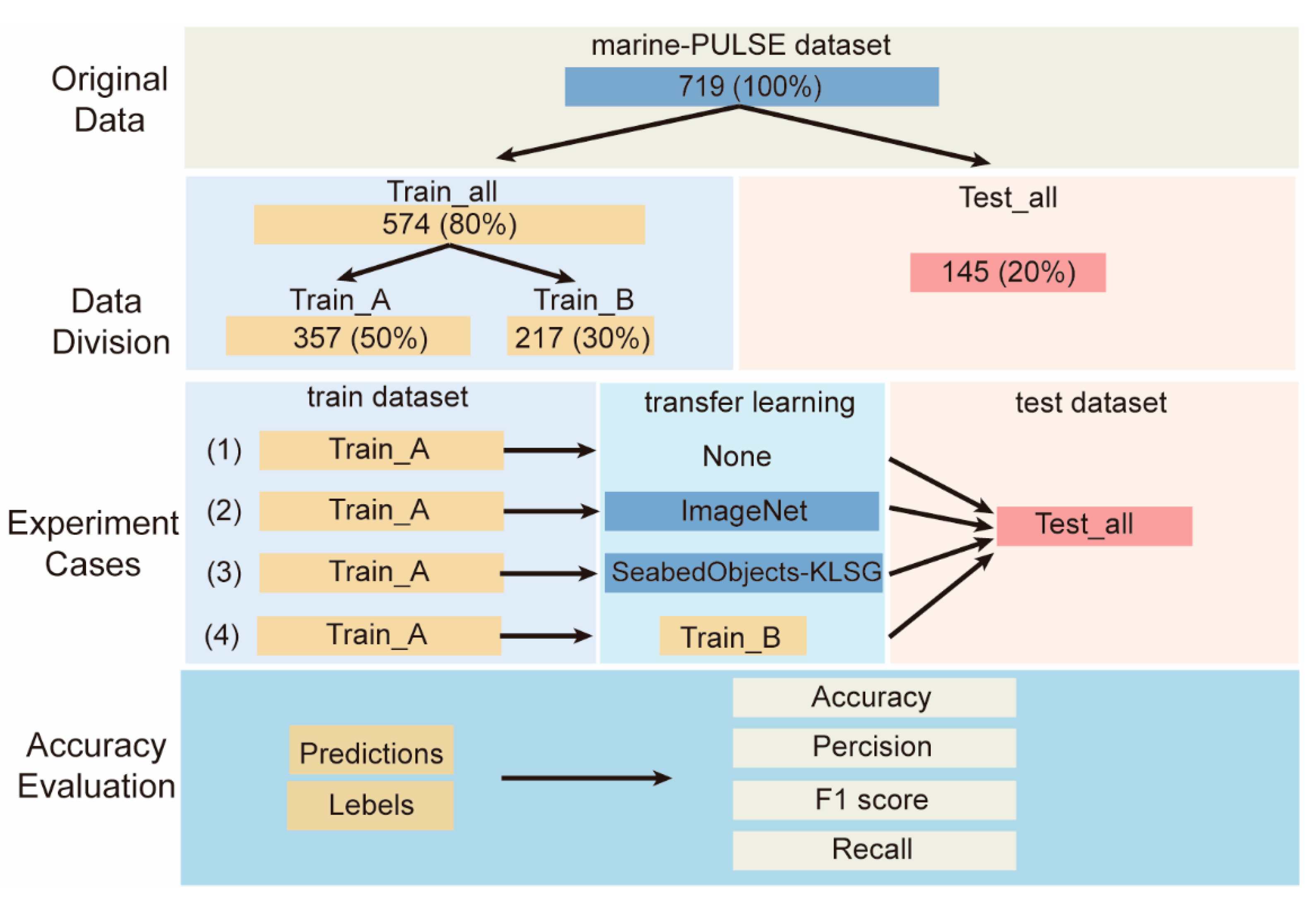
3.2. Experimental Steps

As displayed in Figure 3, we partitioned the Marine-PULSE dataset into two sections, train_all and test_all, following an 80%:20% split. Further, we divided the train_all portion into two distinct subsets: train_A (50%) and train_B (30%). The depicted experimental configuration involved utilizing identical training and testing datasets while varying the pre-training datasets. The training dataset consisted of the labeled samples used to train the model, while the testing dataset served to assess the model’s performance on unseen data. Through the exploration of these four experimental configurations, our goal was to investigate the effects of transfer learning and the choice of pre-training datasets on the model’s performance and generalization capabilities, particularly in the context of the Marine-PULSE dataset.

Before initiating the model training process, it was crucial to carry out data preprocessing and augmentation operations. These operations involved modifying and augmenting the input data in several ways, aiming to enhance the model’s capacity to learn and generalize from the available dataset. By performing these operations, we could significantly improve both the training efficiency and the overall model accuracy.

3.2.1. Data Preprocessing

Prior to the computational modeling, the side-scan sonar (SSS) images were subjected to a sequence of preprocessing operations to align with the input requirements of the convolutional neural network (CNN) training data. The preprocessing procedures involved center cropping, resizing, normalization, and labeling the images.

To emphasize the underwater objects and minimize the influence of the seabed, it was recommended to apply a center crop to the images, utilizing an image’s center as the point of focus. After cropping, the sonar images were resized uniformly to dimensions of 224 × 224 pixels. This resizing step aligned with the input size specifications of the classical CNN models used in this study.

Normalization was conducted to standardize the data across the three channels of the SSS images, bringing the data within the range of [−1, 1]. This normalization process was undertaken to avoid suboptimal training outcomes that could have been caused by significant variances in the data.

After these preprocessing steps, the SSS data were adequately prepared for training the convolutional neural networks. This enabled the subsequent modeling and analysis of the pipeline or cable (POC) images in the dataset. The labeled and processed images were then ready to be fed into the CNN for model training, paving the way for a comprehensive and accurate analysis of underwater structures.

3.2.2. Data Augmentation

In addition to the data preprocessing steps mentioned earlier, data augmentation strategies were implemented during the training phase. These strategies aimed to prevent the neural networks from fixating on irrelevant features, thereby substantially improving the overall model performance. The data augmentation techniques employed in this study included random horizontal flipping and random rotation within the range of −50° to 50°.

During each training iteration, input images underwent random transformations in accordance with the specified augmentation techniques. These transformations added variability and diversity to the original data, effectively enriching the training dataset and enhancing the accuracy of the trained model. By exposing the neural networks to different perspectives and orientations through random alterations of the input images, the models were encouraged to learn robust and invariant features, thereby improving generalization and overall performance.

The data augmentation techniques not only effectively increased the size and diversity of the training dataset but also better equipped the model to handle real-world variations and complexities. These strategies deterred overfitting to the limited training data and promoted the learning of relevant features, thus contributing significantly to the improved accuracy and reliability of the trained model.

3.2.3. Establishing CNN Models

With the data appropriately prepared, we proceeded to construct the model, following the GoogleNet architecture. A fully connected layer was appended to the model with an output size of 2, corresponding to the classes of POC and Non-POC.

In conducting the experiments for this study, we determined the model hyperparameters by referencing the outcomes of previous experiments conducted by the authors on different datasets, along with those performed on the Marine-PULSE dataset. The model exhibited commendable accuracy with a learning rate of 0.001, a batch size of 64, an epoch count of 100, and utilizing the Adam optimizer for optimization.

Across all four experiments, the models were trained using the train_A dataset and evaluated for accuracy using the test_all dataset. The principal distinction between these experiments was in the application of transfer learning and the use of different pre-training datasets.

In the first experiment, we opted against transfer learning, training the models from scratch with randomly initialized weights. For the second experiment, we utilized the ImageNet dataset to pre-train the models, initializing their weights with those obtained from this pre-training phase before proceeding with further training. In the third and fourth experiments, the SeabedObjects-KLSG and train_B datasets, respectively, were used to pre-train the models. Similar to the second experiment, the weights derived from these pre-training stages were used as the initial weights for the subsequent training.

The key distinguishing factor among these experimental setups was the choice of pre-training datasets. Each test explored a different pre-training dataset to initialize the model’s weights before additional training. By leveraging different pre-training datasets, we sought to evaluate their respective impacts on the performance and generalization capabilities of the model.

3.2.4. Model Evaluation

In order to assess the accuracy of GoogleNet in automatically recognizing underwater pipeline objects in SSS images, we employed four evaluation metrics: accuracy, precision, recall, and F1 score. Accuracy measured the overall correctness of the model’s predictions, indicating the proportion of correctly classified instances. Precision quantified the model’s ability to accurately identify positive instances, measuring the proportion of true positive predictions over the total predicted positive instances. Recall assessed the model’s capability to capture all positive instances, indicating the ratio of true positive predictions to the total number of actual positive instances. The F1 score combined precision and recall into a single value, providing a balanced measure that accounted for both precision and recall. These metrics collectively offered a comprehensive evaluation of the model’s accuracy, precision, recall, and overall performance in the recognition of underwater pipeline objects in SSS images. The formulas for the evaluation metrics are as follows:

$$\mathrm{A}\mathrm{c}\mathrm{c}\mathrm{u}\mathrm{r}\mathrm{a}\mathrm{c}\mathrm{y}=(\mathrm{T}\mathrm{P}+\mathrm{T}\mathrm{N})/(\mathrm{T}\mathrm{P}+\mathrm{T}\mathrm{N}+\mathrm{F}\mathrm{P}+\mathrm{F}\mathrm{N})$$

(1)

$$\mathrm{P}\mathrm{r}\mathrm{e}\mathrm{c}\mathrm{i}\mathrm{s}\mathrm{i}\mathrm{o}\mathrm{n}=\mathrm{T}\mathrm{P}/(\mathrm{T}\mathrm{P}+\mathrm{F}\mathrm{P})$$

(2)

$$\mathrm{R}\mathrm{e}\mathrm{c}\mathrm{a}\mathrm{l}\mathrm{l}=\mathrm{T}\mathrm{P}/(\mathrm{T}\mathrm{P}+\mathrm{F}\mathrm{N})$$

(3)

$$\mathrm{F}1 \mathrm{s}\mathrm{c}\mathrm{o}\mathrm{r}\mathrm{e}=2\times (\mathrm{P}\mathrm{r}\mathrm{e}\mathrm{c}\mathrm{i}\mathrm{s}\mathrm{i}\mathrm{o}\mathrm{n}\times \mathrm{R}\mathrm{e}\mathrm{c}\mathrm{a}\mathrm{l}\mathrm{l})/(\mathrm{P}\mathrm{r}\mathrm{e}\mathrm{c}\mathrm{i}\mathrm{s}\mathrm{i}\mathrm{o}\mathrm{n}+\mathrm{R}\mathrm{e}\mathrm{c}\mathrm{a}\mathrm{l}\mathrm{l})$$

(4)

where the representations of TP, TN, FP, and FN can be seen in

Table 1. Confusion matrix for binary classification of POC and Non-POC.

Predicted Label/True Label	Positive Sample (POC)	Negative Sample (Non-POC)
Positive Sample (POC)	TP	FN
Negative Sample (Non-POC)	FP	TN 1

¹ In the binary classification of this study, POC is defined as a positive sample and Non-POC is defined as a negative sample. TP (true positive) denotes the number of POCs correctly classified as POCs. TN (true negative) represents the number of Non-POCs correctly classified as Non-POCs. FP (false positive) indicates the number of Non-POCs incorrectly classified as POCs. FN (false negative) signifies the number of POCs incorrectly classified as Non-POCs.

.

By considering these four elements, we could assess not only the overall accuracy of the model but also its precision (its ability to avoid false positives) and its recall (its ability to avoid false negatives). The F1 score provided a balanced view that considered both precision and recall.

Analyzing these metrics can indeed provide valuable insights into the performance of GoogleNet in recognizing underwater pipeline objects in SSS images. These metrics can help determine the model’s strengths and identify areas where improvement may be needed, thereby assisting in optimizing the model’s performance in future iterations or similar tasks.

3.3. Experimental Environment

All the code for the calculation was implemented in the deep learning modeling package Pytorch. The calculating device was a workstation with an Intel i9-12900K CPU, 128 G of RAM, and an NVIDIA RTX 4090 graphics card.

4. Results and Analysis

4.1. Accuracy of GoogleNet for SSS Image Recognition of POCs

Utilizing GoogleNet as our foundational model, we initialized our training process with pre-training weights derived from the ImageNet dataset. As illustrated in Figure 4a, a noticeable enhancement in the model’s accuracy was recorded over the course of 100 training epochs. The model’s accuracy on the test dataset started at 65% and notably increased to over 90% within 20 epochs, emphasizing a substantial improvement in its predictive capabilities. After the 20-epoch milestone, the accuracy fluctuated but still maintained a commendable performance, with the peak accuracy exceeding 90%.

Figure 4b,c depict the evolution of the precision and recall metrics, respectively, throughout the training process. Both metrics exhibited a sharp incline as the number of epochs progressed, indicating a growing improvement in the model’s ability to accurately identify true positives (precision) and correctly recall actual positive instances (recall). The F1 score, a metric that harmonizes precision and recall, echoed these observations, showing a comparable upward trend.

This extensive analysis of accuracy, precision, recall, and the F1 score clearly substantiated the efficacy of the GoogleNet model in accurately classifying SSS images of Potential Objects of Concern (POCs). The model demonstrated a prediction accuracy exceeding 90%, a remarkable performance that underscores the strength of transfer learning in this application. The usage of pre-trained weights from the ImageNet dataset allowed the model to leverage previously learned patterns and features, thus contributing significantly to its high performance.

In summary, the results reaffirm the potential of transfer learning in enhancing the predictive performance of machine learning models, particularly in scenarios of marine geological problems where the task involves recognizing complex underwater structures in side-scan sonar images. These findings could have significant implications for the wider field of marine engineering and could pave the way for more efficient and effective inspections of underwater structures, thus contributing to improved safety and maintenance practices.

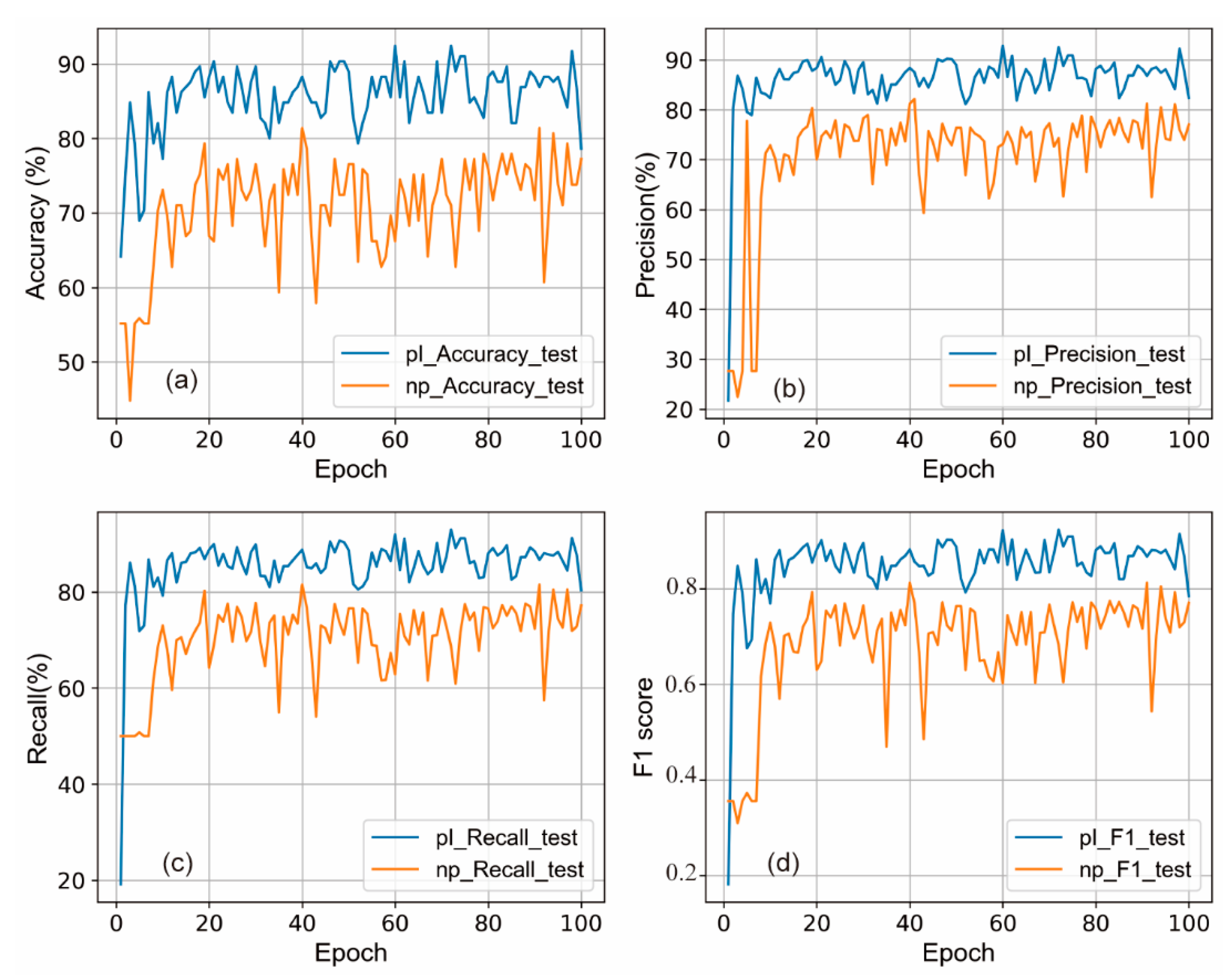
4.2. Model Performance with and without Transfer Learning

To understand the influence of transfer learning (TL) on the accuracy of POC image predictions, we conducted a comparative analysis between models using TL with pre-training on the ImageNet dataset and models without TL.

From the results presented in Figure 5a, we observed that the accuracy of the model without transfer learning plateaued at a maximum of 80% and exhibited no substantial increase beyond 20 epochs. This level of accuracy was noticeably lower than the prediction accuracy achieved by the model employing pre-training. Similarly, Figure 5b–d reveal that the model trained without transfer learning significantly underperformed in precision, recall, and F1 score values when compared to the model that used pre-training.

Therefore, it is apparent that the application of transfer learning played a vital role in enhancing the model’s predictive capabilities. By leveraging the pre-trained weights from ImageNet, the model benefited from the knowledge and patterns already captured, which are typically applicable across various domains or tasks. This strategy contributed to faster convergence, higher accuracy, and improved generalization in the context of the Marine-PULSE dataset, as it aided the model in better understanding and interpreting SSS images of POCs.

The results suggest that transfer learning, particularly pre-training on large and diverse datasets like ImageNet, is a highly beneficial strategy in submarine pipeline object recognition tasks. This approach could be further explored and could be employed in other related tasks in marine imaging and underwater object recognition. This could also prompt further exploration into more robust and efficient transfer learning techniques and their application in different areas within the field of marine science.

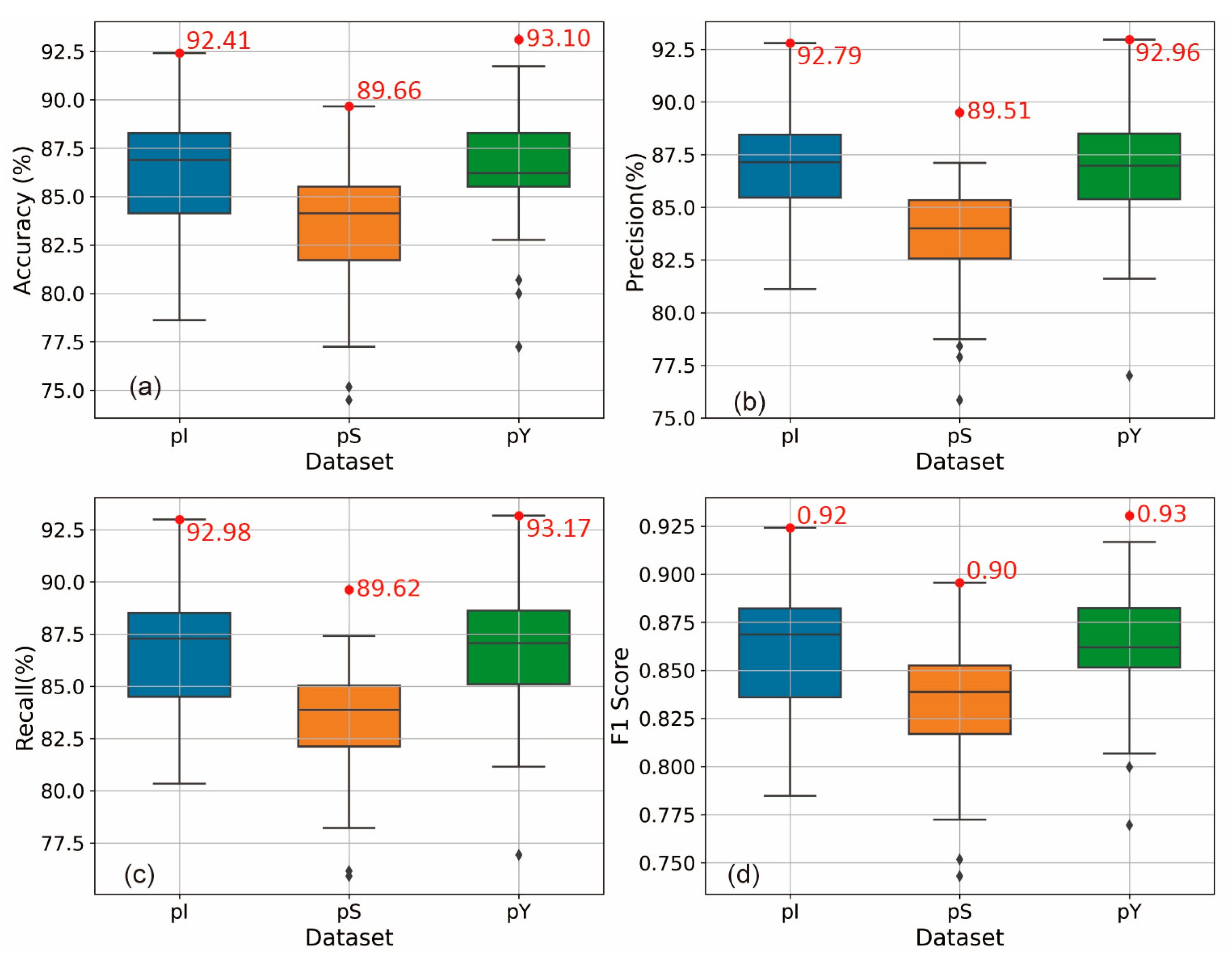
4.3. Performance Comparison Using Different Pre-Training Datasets

The role of pre-training datasets in transfer learning cannot be overstated. Selecting an appropriate pre-training dataset can contribute rich feature representations and enhance the generalization capabilities of a model, equipping it with valuable prior knowledge applicable to the target task. By incorporating pre-training datasets, a model can learn generic features, allowing it to converge faster and adapt more effectively to new data. Factors such as the task’s characteristics, data similarity, data diversity, and available computational resources should be considered when choosing pre-training datasets, as they lay a solid foundation for successful transfer learning.

In our study, we selected ImageNet, SeabedObjects-KLSG, and a subset of the Marine-PULSE dataset (train_B) for pre-training. The weights from these pre-trained models were utilized as the initial weights for subsequent training. The goal was to investigate the impact of different pre-training datasets on the recognition of side-scan sonar (SSS) images of Potential Objects of Concern (POCs).

As depicted in Figure 6, with the progression of the epochs, the evaluation metrics for all three models increased rapidly, reaching a relatively stable state after around 20 epochs. Among the three models, the one pre-trained with the SeabedObjects-KLSG dataset performed the least effectively in prediction, as suggested by all four evaluation metrics. Conversely, the models pre-trained with ImageNet and a subset, named train_B, of the Marine-PULSE dataset showed similar performances, with no clearly discernable difference in Figure 6.

These findings highlight the importance of pre-training dataset selection in transfer learning applications. While the SeabedObjects-KLSG dataset did not yield high-performing models in this context, both the ImageNet and Marine-PULSE datasets provided effective pre-training, resulting in models with high accuracy, precision, recall, and F1 scores. This implies that datasets with features more closely resembling those of the target task could result in improved model performance, emphasizing the importance of data similarity and diversity in pre-training dataset selection.

To conduct a more comprehensive comparison and analysis of the predictive results of the three models, we conducted a statistical analysis of the prediction outcomes from the 50th epoch to the 100th epoch, after the models had reached a stable state. This analysis aimed to compare the statistical distribution characteristics of the results.

As shown in Figure 7a, the models pre-trained on ImageNet (pI) exhibited the highest median accuracy, with a closely grouped distribution indicating consistent performance. On the other hand, the Marine-PULSE (pY)-pre-trained model demonstrated a slightly lower median accuracy with a wider distribution, indicating some variability in its predictions. Lastly, the SeabedObjects-KLSG (pS)-pre-trained model showed the lowest accuracy, with a more scattered distribution.

Upon examining Figure 7b, we observed that the ImageNet (pI)-pre-trained models once again outperformed, with the highest median precision and a tightly packed distribution. The Marine-PULSE (pY)-pre-trained model showed a marginally lower median precision with a broader distribution. Meanwhile, the models pre-trained on SeabedObjects-KLSG (pS) displayed the lowest precision with a more expansive distribution.

As per Figure 7c, the Marine-PULSE (pY)-pre-trained model had the highest median recall with a tighter distribution, suggesting consistent identification of relevant instances. The ImageNet (pI)-pre-trained models had a slightly lower median recall but demonstrated a wider distribution. The SeabedObjects-KLSG (pS)-pre-trained models exhibited the lowest recall with a broad distribution.

Figure 7d reveals that the ImageNet (pI)-pre-trained models achieved the highest median F1 score, indicating a balanced precision and recall, with a narrow distribution. The Marine-PULSE (pY)-pre-trained model showed a slightly lower median F1 score with a more dispersed distribution. Finally, the models pre-trained on SeabedObjects-KLSG (pS) achieved the lowest F1 score with a wider distribution.

To summarize, the choice of pre-training dataset significantly influenced the predictive performance of the model, as evident from the data presented in Figure 7. When evaluating the predictive effectiveness of deep learning models, it is crucial to consider both the stability of the results across multiple trials and the maximum accuracy. In terms of maximum accuracy, Marine-PULSE (pY) provided the highest results for all four metrics, closely followed by ImageNet (pI). Among the three pre-training datasets, ImageNet (pI) yielded stable and effective pre-training results across repeated trials and Marine-PULSE (pY) produced similar results, whereas the SeabedObjects-KLSG (pS) results diverged more from the other two datasets. These results underscore the critical role of pre-training dataset selection in transfer learning for deep learning models.

The disparities among the datasets significantly influenced model performance. ImageNet, with its diverse and extensive data, endowed the model with rich feature representations, enhancing its generalization. However, its low consistency with SSS images of the seafloor was a limitation. Marine-PULSE, while smaller, had high consistency with the target task, proving that similarity between pre-training and target data is crucial for model efficacy. Its performance was comparable to ImageNet, demonstrating that dataset relevance can sometimes outweigh volume. Conversely, SeabedObjects-KLSG, despite its relevance in content, lagged in performance, highlighting the importance of both data diversity and relevance. These disparities underscore the necessity of careful dataset selection in transfer learning applications, balancing diversity, volume, and task relevance to optimize model performance.

5. Discussion

Our analysis of the prediction accuracy, precision, recall, and F1 scores allowed us to evaluate the performance of the various CNN models discussed in this paper. The results indicated that GoogleNet can accurately predict SSS images of POCs. Moreover, we observed that different pre-training datasets influenced the model’s predictive outcomes. This variation is likely associated with the types of images in a dataset, the number of images, and their consistency with the research problem.

The ImageNet dataset, with its wide range of image types and categories, enabled the model to learn a richer feature representation, demonstrating good applicability and stability. The Marine-PULSE dataset, likely due to its closer similarity to the data distribution of the target task, achieved the highest accuracy rate, albeit with slightly fluctuating stability in repeated trials. Conversely, the SeabedObjects-KLSG (pS) dataset, being quite dissimilar from the POC prediction and lacking sufficiently diverse categories and the numbers to provide generalization performance, demonstrated the least effectiveness among the three datasets.

As seen in

Table 2. Comparison of data, types of different pre-training datasets.

Dataset	Types/Categories	Volume/Size	Consistency 1
ImageNet	1000	150 GB	Low
SeabedObjects-KLSG	2	67.5 M	Median
Marine-PULSE (train_B)	2	22.2 M	Very High

¹ Consistency represents the relevant similarity between the pre-training and predicted data.

, ImageNet, with its 1000 types of images, could essentially cover all data types under study. However, its consistency was low because its images were mainly derived from various types of objects or organisms, which are vastly different from the side-scan sonar images of the seafloor. Despite this, due to the extensive amount of data in ImageNet (150 GB), the model was trained to produce good generalization. Therefore, even with low consistency, the richness of model variety and the large amount of data compensated for this deficiency, resulting in good predictive outcomes.

Regarding the SeabedObjects-KLSG dataset, despite it having two types of side-scan sonar images (plane and ship) and being somewhat consistent with the study as it involves side-scan sonar images, the prediction results using this dataset for pre-training significantly lagged behind the other two datasets. This can be attributed to the fact that its image types were quite different from POCs and thus could not contribute valid information for the learning process. Only the common information across side-scan sonar images could be learned.

The train_B dataset, comprising a random 20% of the data from the Marine-PULSE dataset, had high consistency with the final images to be predicted. Even with only 22.2 MB of data, it provided the model with sufficient information for pre-training. Consequently, this dataset achieved a similar pre-training effect as ImageNet’s 150 GB data volume, despite its considerably smaller size.

However, it is important to understand that this result is specific to the prediction of POCs using SSS images. The Marine-PULSE dataset, while achieving a similar prediction performance as ImageNet with about 1/6900 of the data volume, may not replicate such favorable outcomes for other marine geological image prediction tasks. For different seafloor side-scan sonar image predictions, it might yield results akin to those of the SeabedObjects-KLSG dataset—surpassing models without pre-training but falling short of models pre-trained with ImageNet.

Regarding the deep learning model we used in this study, there are two disadvantages to note: generalization and model complexity. While GoogleNet performed admirably on our Marine-PULSE dataset, its generalization capability for other types of marine geological and geophysical data needs further investigation and validation. Despite its computational efficiency, GoogleNet’s complex architecture might still be resource-intensive for real-time applications on board marine exploration vessels, where computational resources could be limited.

Consequently, for future image recognition problems, we recommend collecting images with high consistency with the predicted images for pre-training to improve the prediction performance of the final model. When there are no consistent images for pre-training, a more general dataset like ImageNet could be an effective choice.

6. Conclusions

In this study, we utilized GoogleNet to automatically recognize SSS images of POCs, thereby exploring the feasibility of using CNN models for POC prediction. We also assessed the impact of transfer learning on model accuracy and used three distinct datasets for pre-training to examine the influence of different datasets on model accuracy. The principal findings are as follows:

(1)

Utilizing GoogleNet modeling permitted efficient identification of SSS images of underwater pipelines, with accuracy and precision rates exceeding 90%.

(2)

Transfer learning significantly enhanced the accuracy of the model. The model could reach up to 80% accuracy without pre-training. Following pre-training with the ImageNet dataset, the model’s prediction accuracy could be boosted by approximately 10% compared to when there was no pre-training.

(3)

Different pre-training datasets yielded varying impacts on model prediction accuracy. The datasets that enhanced the model prediction ability, ranked in descending order of effectiveness, were Marine-PULSE, ImageNet, and SeabedObjects-KLSG.

(4)

The type of pre-training dataset, the volume of data, and the consistency with the predicted data are crucial factors influencing the pre-training effect. When the consistency is very high, even a minimal amount of data can yield a satisfactory pre-training effect. Conversely, when consistency is low, a dataset with a large volume of data and good generalization should be selected.

There are also some inherent limitations in the current study. The findings pertaining to the impact of transfer learning datasets are specific to SSS images of undersea pipelines. Their general applicability to other domains or marine objects remains unvalidated and warrants further investigation. In the future, we will aim to expand the horizons of this study by testing our methodologies across a broader spectrum of marine data and scenarios. By doing so, we intend to further ascertain the universal applicability and robustness of the described methodologies.

References

1. Gašparović, B.; Lerga, J.; Mauša, G.; Ivašić-Kos, M. Deep Learning Approach For Objects Detection in Underwater Pipeline Images. Appl. Artif. Intell. 2022, 36, 2146853. [Google Scholar] [CrossRef]
2. Sung, M.; Kim, J.; Lee, M.; Kim, B.; Kim, T.; Kim, J.; Yu, S.-C. Realistic Sonar Image Simulation Using Deep Learning for Underwater Object Detection. Int. J. Control Autom. Syst. 2020, 18, 523–534. [Google Scholar] [CrossRef]
3. Wang, H.; Gao, N.; Xiao, Y.; Tang, Y. Image Feature Extraction Based on Improved FCN for UUV Side-Scan Sonar. Mar. Geophys. Res. 2020, 41, 18. [Google Scholar] [CrossRef]
4. Fan, X.; Lu, L.; Shi, P.; Zhang, X. A Novel Sonar Target Detection and Classification Algorithm. Multimed. Tools Appl. 2022, 81, 10091–10106. [Google Scholar] [CrossRef]
5. Pouyan, S.; Pourghasemi, H.R.; Bordbar, M.; Rahmanian, S.; Clague, J.J. A Multi-Hazard Map-Based Flooding, Gully Erosion, Forest Fires, and Earthquakes in Iran. Sci. Rep. 2021, 11, 14889. [Google Scholar] [CrossRef]
6. St. Denis, L.A.; Short, K.C.; McConnell, K.; Cook, M.C.; Mietkiewicz, N.P.; Buckland, M.; Balch, J.K. All-Hazards Dataset Mined from the US National Incident Management System 1999–2020. Sci. Data 2023, 10, 112. [Google Scholar] [CrossRef]
7. Zhao, C.; Lu, Z. Remote Sensing of Landslides—A Review. Remote Sens. 2018, 10, 279. [Google Scholar] [CrossRef]
8. Xu, S.; Dimasaka, J.; Wald, D.J.; Noh, H.Y. Seismic Multi-Hazard and Impact Estimation via Causal Inference from Satellite Imagery. Nat. Commun. 2022, 13, 7793. [Google Scholar] [CrossRef]
9. Stanley, T.A.; Kirschbaum, D.B.; Sobieszczyk, S.; Jasinski, M.F.; Borak, J.S.; Slaughter, S.L. Building a Landslide Hazard Indicator with Machine Learning and Land Surface Models. Environ. Model. Softw. 2020, 129, 104692. [Google Scholar] [CrossRef]
10. Ma, Z.; Mei, G. Deep Learning for Geological Hazards Analysis: Data, Models, Applications, and Opportunities. Earth-Sci. Rev. 2021, 223, 103858. [Google Scholar] [CrossRef]
11. Mousavi, S.M.; Ellsworth, W.; Weiqiang, Z.; Chuang, L.; Beroza, G. Earthquake Transformer—An Attentive Deep-Learning Model for Simultaneous Earthquake Detection and Phase Picking. Nat. Commun. 2020, 11, 3952. [Google Scholar] [CrossRef]
12. Rateria, G.; Maurer, B.W. Evaluation and Updating of Ishihara’s (1985) Model for Liquefaction Surface Expression, with Insights from Machine and Deep Learning. Soils Found. 2022, 62, 101131. [Google Scholar] [CrossRef]
13. Jones, S.; Kasthurba, A.K.; Bhagyanathan, A.; Binoy, B.V. Landslide Susceptibility Investigation for Idukki District of Kerala Using Regression Analysis and Machine Learning. Arab. J. Geosci. 2021, 14, 838. [Google Scholar] [CrossRef]
14. Chang, Z.; Du, Z.; Zhang, F.; Huang, F.; Chen, J.; Li, W.; Guo, Z. Landslide Susceptibility Prediction Based on Remote Sensing Images and GIS: Comparisons of Supervised and Unsupervised Machine Learning Models. Remote Sens. 2020, 12, 502. [Google Scholar] [CrossRef]
15. Jena, R.; Pradhan, B.; Beydoun, G.; Al-Amri, A.; Sofyan, H. Seismic Hazard and Risk Assessment: A Review of State-of-the-Art Traditional and GIS Models. Arab. J. Geosci. 2020, 13, 50. [Google Scholar] [CrossRef]
16. Du, X.; Sun, Y.; Song, Y.; Xiu, Z.; Su, Z. Submarine Landslide Susceptibility and Spatial Distribution Using Different Unsupervised Machine Learning Models. Appl. Sci. 2022, 12, 10544. [Google Scholar] [CrossRef]
17. Abadi, S. Using Machine Learning in Ocean Noise Analysis during Marine Seismic Reflection Surveys. J. Acoust. Soc. Am. 2018, 144, 1744. [Google Scholar] [CrossRef]
18. Chandrashekar, G.; Raaza, A.; Rajendran, V.; Ravikumar, D. Side Scan Sonar Image Augmentation for Sediment Classification Using Deep Learning Based Transfer Learning Approach. Mater. Today Proc. 2023, 80, 3263–3273. [Google Scholar] [CrossRef]
19. Nayak, N.; Nara, M.; Gambin, T.; Wood, Z.; Clark, C.M. Machine Learning Techniques for AUV Side-Scan Sonar Data Feature Extraction as Applied to Intelligent Search for Underwater Archaeological Sites. In Proceedings of the Field and Service Robotics; Ishigami, G., Yoshida, K., Eds.; Springer: Singapore, 2021; pp. 219–233. [Google Scholar]
20. Pillay, T.; Cawthra, H.C.; Lombard, A.T. Integration of Machine Learning Using Hydroacoustic Techniques and Sediment Sampling to Refine Substrate Description in the Western Cape, South Africa. Mar. Geol. 2021, 440, 106599. [Google Scholar] [CrossRef]
21. Juliani, C.; Juliani, E. Deep Learning of Terrain Morphology and Pattern Discovery via Network-Based Representational Similarity Analysis for Deep-Sea Mineral Exploration. Ore Geol. Rev. 2021, 129, 103936. [Google Scholar] [CrossRef]
22. Pillay, T.; Cawthra, H.C.; Lombard, A.T. Characterisation of Seafloor Substrate Using Advanced Processing of Multibeam Bathymetry, Backscatter, and Sidescan Sonar in Table Bay, South Africa. Mar. Geol. 2020, 429, 106332. [Google Scholar] [CrossRef]
23. Sircar, A.; Yadav, K.; Rayavarapu, K.; Bist, N.; Oza, H. Application of Machine Learning and Artificial Intelligence in Oil and Gas Industry. Pet. Res. 2021, 6, 379–391. [Google Scholar] [CrossRef]
24. Jin, L.; Liang, H.; Yang, C. Accurate Underwater ATR in Forward-Looking Sonar Imagery Using Deep Convolutional Neural Networks. IEEE Access 2019, 7, 125522–125531. [Google Scholar] [CrossRef]
25. Yulin, T.; Jin, S.; Bian, G.; Zhang, Y. Shipwreck Target Recognition in Side-Scan Sonar Images by Improved YOLOv3 Model Based on Transfer Learning. IEEE Access 2020, 8, 173450–173460. [Google Scholar] [CrossRef]
26. Zhu, B.; Wang, X.; Chu, Z.; Yang, Y.; Shi, J. Active Learning for Recognition of Shipwreck Target in Side-Scan Sonar Image. Remote Sens. 2019, 11, 243. [Google Scholar] [CrossRef]
27. Xiong, C.; Lian, S.; Chen, W. An Ensemble Method for Automatic Real-Time Detection, Evaluation and Position of Exposed Subsea Pipelines Based on 3D Real-Time Sonar System. J. Civil Struct. Health Monit. 2023, 13, 485–504. [Google Scholar] [CrossRef]
28. Yan, J.; Meng, J.; Zhao, J. Bottom Detection from Backscatter Data of Conventional Side Scan Sonars through 1D-UNet. Remote Sens. 2021, 13, 1024. [Google Scholar] [CrossRef]
29. Sun, Y.; Zheng, H.; Zhang, G.; Ren, J.; Xu, H.; Xu, C. DP-ViT: A Dual-Path Vision Transformer for Real-Time Sonar Target Detection. Remote Sens. 2022, 14, 5807. [Google Scholar] [CrossRef]
30. Du, X.; Sun, Y.; Song, Y.; Sun, H.; Yang, L. A Comparative Study of Different CNN Models and Transfer Learning Effect for Underwater Object Classification in Side-Scan Sonar Images. Remote Sens. 2023, 15, 593. [Google Scholar] [CrossRef]
31. Huo, G.; Wu, Z.; Li, J. Underwater Object Classification in Sidescan Sonar Images Using Deep Transfer Learning and Semisynthetic Training Data. IEEE Access 2020, 8, 47407–47418. [Google Scholar] [CrossRef]
32. Szegedy, C.; Liu, W.; Jia, Y.; Sermanet, P.; Reed, S.; Anguelov, D.; Erhan, D.; Vanhoucke, V.; Rabinovich, A. Going Deeper with Convolutions. arXiv 2014, arXiv:1409.4842. [Google Scholar]
33. Bousmalis, K.; Trigeorgis, G.; Silberman, N.; Krishnan, D.; Erhan, D. Domain Separation Networks. arXiv 2016, arXiv:1608.06019. [Google Scholar]
34. Pires de Lima, R.; Marfurt, K. Convolutional Neural Network for Remote-Sensing Scene Classification: Transfer Learning Analysis. Remote Sens. 2020, 12, 86. [Google Scholar] [CrossRef]
35. Rostami, M.; Kolouri, S.; Eaton, E.; Kim, K. Deep Transfer Learning for Few-Shot SAR Image Classification. Remote Sens. 2019, 11, 1374. [Google Scholar] [CrossRef]
36. Koga, Y.; Miyazaki, H.; Shibasaki, R. A Method for Vehicle Detection in High-Resolution Satellite Images That Uses a Region-Based Object Detector and Unsupervised Domain Adaptation. Remote Sens. 2020, 12, 575. [Google Scholar] [CrossRef]
37. Du, X. Side-Scan Sonar Images of Marine Engineering Geology (Marine_PULSE Dataset); Zenodo: Geneva, Switzerland, 2023. [Google Scholar]
Figure 1. Structure of Inception [30].
Remotesensing 15 04873 g001
Figure 2. Samples from the Marine-PULSE dataset. Samples in rows (ad) are pipelines or cables, underwater residual mounds, seabed surface, and engineering platforms, respectively.
Remotesensing 15 04873 g002
Figure 3. Flow chart of data division, experiment cases, and accuracy evaluation.
Remotesensing 15 04873 g003
Figure 4. Variation in prediction evaluation metrics of the model in the test dataset over 100 epochs. (a) Accuracy; (b) precision; (c) recall; (d) F1 score.
Remotesensing 15 04873 g004
Figure 5. The effect of transfer learning on the prediction accuracy of different CNN models on the test dataset. pI = pre-training with ImageNet dataset; np = no pre-training. (ad) represent the accuracy, precision, recall, and F1 score of the model’s calculations with and without transfer learing, respectively.
Remotesensing 15 04873 g005
Figure 6. Variation in prediction evaluation metrics over 100 epochs in the test set using models with different training datasets. pI = pre-training with ImageNet dataset; pS = pre-training with SeabedObjects-KLSG dataset; pS = pre-training with train_B from Marine-PULSE dataset. (ad) represent the accuracy, precision, recall, and F1 score of the model computation results using the pI, pS, and pY pretraining datasets, respectively.
Remotesensing 15 04873 g006
Figure 7. Statistics of prediction evaluation metrics in the test set using models different from the training dataset. pI = pre-training with ImageNet dataset; pS = pre-training with SeabedObjects-KLSG dataset; pS = pre-training with train_B from Marine-PULSE dataset. The last 50 epochs of the model predictions were used for statistical analysis. The red dots indicate the maximum values of the 50 sets of predicted results. (ad) represent the statistical analysis of accuracy, precision, recall, and F1 score of the model computation results using the pI, pS, and pY pretraining datasets, respectively.
Remotesensing 15 04873 g007