Retrievals of Chlorophyll-a from GOCI and GOCI-II Data in Optically Complex Lakes

Abstract

The chlorophyll-a (Chla) concentration is a key parameter to evaluate the eutrophication conditions of water, which is very important for monitoring algal blooms. Although Geostationary Ocean Color Imager (GOCI) has been widely used in Chla inversion, the consistency of the Rayleigh-corrected reflectance (R_rc) of GOCI and GOCI-II sensors still needs to be further evaluated, and a model suitable for lakes with complex optical properties needs to be constructed. The results show that (1) the derived Chla values of the GOCI and GOCI-II synchronous data were relatively consistent and continuous in three lakes in China. (2) The accuracy of the random forest (RF) model (R² = 0.84, root mean square error (RMSE) =11.77 μg/L) was higher than that of the empirical model (R² = 0.79, RMSE = 12.63 μg/L) based on the alternative floating algae index (AFAI). (3) The interannual variation trend fluctuated, with high Chla levels in Lake Chaohu in 2015 and 2019, while those in Lake Hongze were high in 2013, 2015, and 2022, and those in Lake Taihu reached their peak in 2017 and 2019. There were three types of diurnal variation patterns, namely, near-continuous increase (Class 1), near-continuous decrease (Class 2), and first an increase and then a decrease (Class 3), among which Lake Chaohu and Lake Taihu occupied the highest proportion in Class 3. The results analyzed the temporal and spatial variations of Chla in three lakes for 12 years and provided support for the use of GOCI and GOCI-II data and monitoring of Chla in optical complex inland waters.

1. Introduction

Chlorophyll-a is a common pigment in phytoplankton, and its concentration is an important parameter to describe the nutritional status of water, which is the focus of lake environment quality assessment studies [1]. Traditional water quality monitoring is a time-consuming and labor-intensive task, and it is difficult to monitor the water quality on a large spatial scale [2]. With the development of remote sensing technology and the continuous launch of water color satellites, the differences in the optical properties of natural water caused by phytoplankton pigments, suspended particulate matter (SPM), and colored dissolved organic matter (CDOM) are reflected in remote sensing spectral signals [3]. This provides the possibility for multiscale monitoring in time and space and is very important for lake environment management and ecological protection.

Because of the advantages of easy acquisition and fast image processing, satellites are widely used in the quantitative inversion of Chla. The multispectral satellite data used in inversion include Landsat series data [4], Moderate Resolution Imaging Spectroradiometer (MODIS) data [5], Sentinel series data [6], Medium Resolution Imaging Spectrometer (MERIS) data [7], GOCI data [8], Visible Infrared Imager Radiometer Suite (VIIRS) data [9], and GF-1 Wide Field of View (WFV) data [10]. The inversion algorithms for Chla mainly include empirical, semi-analytical, and analytical algorithms [11]. In recent years, machine learning models, such as the neural network (NN) [12] algorithm, extreme gradient boosting (XGBoost) algorithm, support vector regression (SVR) model [13], and random forest (RF) model [14], have also been widely used in the inversion of Chla, and a satisfactory performance has been achieved. Among them, the random forest model exhibits the characteristics of high accuracy and high speed [15].

However, influenced by the wind speed, wind direction, precipitation, diurnal variations in algae, and other factors, Chla may change rapidly in a day or even a few hours [16]. Thus, satellites with moderate or low temporal resolution can hardly meet the needs of high-frequency monitoring. In comparison, the GOCI sensor carried by the Communication, Ocean, and Meteorological Satellite (COMS) provides a higher temporal resolution (1 h) and signal-to-noise ratio, which can reduce the effect of missing data due to cloud interference. Previous studies have used GOCI data to estimate Chla in Lake Taihu [17], determine SPM in Lake Hongze [18], and observe cyanobacteria blooms in Lake Taihu [19]. Although the GOCI sensor stopped operating in March 2021, GEO-KOMPSAT-2B (GK-2B) was successfully launched in February 2020, which provides data guarantees for follow-up research. The time coverage and imaging bands of the GOCI-II sensor were increased, making it more suitable for water color research [20]; however, the consistency between the two sensors in estimating Chla must be further confirmed to obtain long-term diurnal observations of Chla.

Lake Chaohu, Lake Hongze, and Lake Taihu are typical lakes with complex optical properties affected by human activities and exhibit serious eutrophication and turbid water quality issues. The aims of this paper were to: (1) evaluate the consistency of GOCI and GOCI-II R_rc data and provide a reference for the use of long-term data series; (2) assess the differences between the empirical model and the random forest model and develop a Chla model suitable for lakes with complex optical properties; and (3) produce temporal and spatial distribution products of Chla in Lake Chaohu, Lake Hongze, and Lake Taihu from 2011 to 2022 and analyze the properties of interannual, monthly, and diurnal variations. This paper is the first to evaluate the consistency of GOCI and GOCI-II data in the inversion of Chla in turbid and eutrophic lakes, which can provide a reference for dynamic Chla monitoring.

2. Materials and Methods

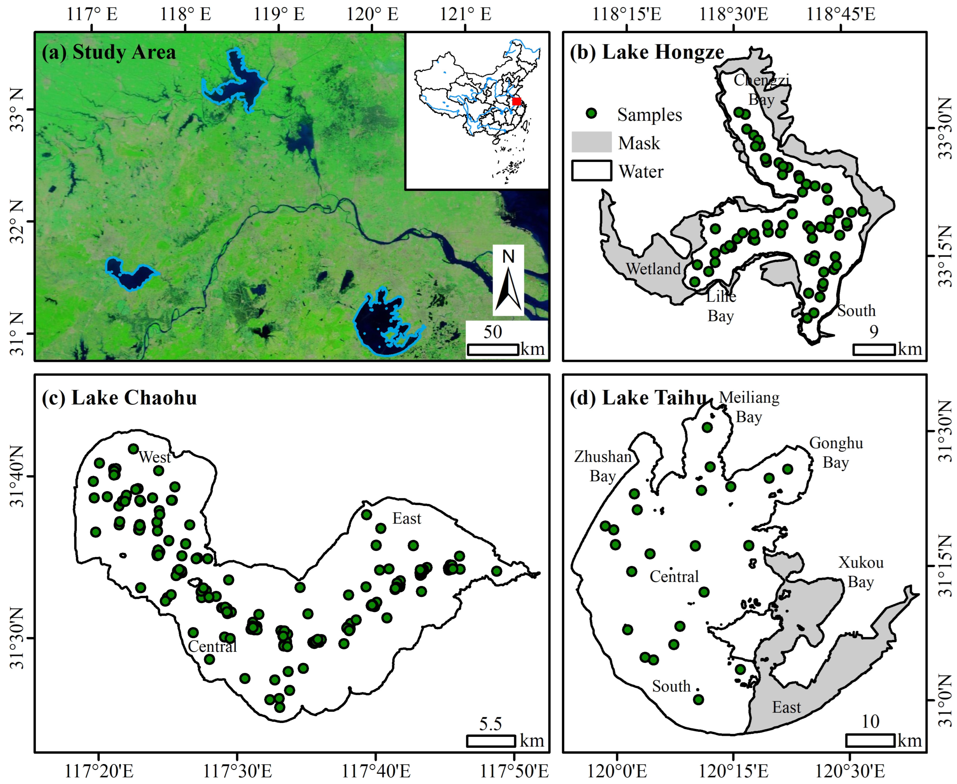
2.1. Study Area

Lake Taihu (2338 km², 30°56′–31°34′N, 119°54′–120°36′N), Lake Hongze (1577 km², 33°06′–33°40′N, 118°10′–118°52′N), and Lake Chaohu (768 km², 31°25′–31°43′N, 117°17′–117°52′N) are the third, fourth, and fifth largest freshwater lakes in China, respectively (Figure 1). The mean water depths are 1.9, 3.0, and 1.9 m, and the mean Secchi disk depths are 0.40, 0.27, and 0.27 m in Lake Taihu, Lake Chaohu, and Lake Hongze, respectively [21]. Xukou Bay and the southeastern part of Lake Taihu mostly contain aquatic vegetation, including emergent, floating-leaved, free-floating, and submerged hydrophytes [22]. Lake Hongze is relatively turbid, and the aquatic vegetation in the western part is widely distributed [23]. To ensure the accuracy of Chla data, the growth range of aquatic vegetation in Lake Taihu and Lake Hongze was masked.

2.2. Water Sampling and Measurements

A total of 54 days were selected for field sampling in Lake Chaohu, Lake Hongze, and Lake Taihu from 2013 to 2018. The water samples were filtered through a GF/F glass fiber membrane with an aperture of 47 mm, and the filter membranes were frozen and soaked in an acetone solution with a concentration of 90% for light-proof extraction. The extraction solution was placed in a colorimetric plate, and the concentration of Chla at the sample site was calculated after the absorbance was measured by a UV2700 (Shimadzu, Tokyo, Japan) spectrophotometer [24].

2.3. Satellite Image Acquisition and Processing

GOCI data were downloaded from the Korea Ocean Satellite Center (KOSC) (http://kosc.kiost.ac.kr/, accessed on 1 June 2022), covering a target area of 2500 km × 2500 km centered on Korea (36°N, 130°E). The area was observed from May 2011 to March 2021, with a spatial resolution of 500 m and a temporal resolution of 1 h, providing 8 field images from 8:16 to 15:16 (UTC + 8). GOCI L1B data covering the three lakes was processed on the SeaDAS (Version 7.5.3) platform and used to derive R_rc by removing Rayleigh scattering signals [25].

The spatial resolution of the GOCI-II sensor has been increased to 250 m, and the number of spectral bands has been increased from 8 to 12 (Figure 2). The satellite transit frequency has been extended to 10 images per day from 7:15 to 16:15 (UTC + 8), which provides higher applicability for monitoring inland lakes. Due to the short online time of GOCI-II data, the SeaDAS platform cannot process first-level data temporarily. Therefore, R_rc data processed by the GOCI-II atmospheric correction (G2AC) algorithm was obtained from the official website (https://www.nosc.go.kr/, accessed on 1 April 2023). G2AC was based on the atmospheric correction algorithm of GOCI and attained favorable performance in both clear and turbid water [26].

Cloudless images for this study region were selected from GOCI and GOCI-II data. The number of available images of Lake Chaohu, Lake Hongze, and Lake Taihu from 2011 to 2022 is shown in Figure 3. Inland water does not meet the assumptions of the standard near-infrared atmospheric correction algorithm, and GOCI lacks a shortwave infrared band [27]; therefore, the accuracy of the existing atmospheric correction methods and effective pixel numbers can hardly satisfy the monitoring needs. Therefore, R_rc was used in this study to build an inversion model for Chla. In addition, to ensure the uniformity of the inversion results, the resolution of the satellite images was resampled to 250 m. To verify the continuity and availability of the two sensors, GOCI and GOCI-II synchronous data were selected for comparison. From January to March 2021, a total of 215 images (77 scenes of Lake Chaohu, 72 scenes of Lake Hongze, and 66 scenes of Lake Taihu) were derived. Match-up pairs within the three lakes were randomly selected with an interval time of less than 1 min, and samples with a CV > 10% were excluded.

2.4. Mask Determination and Match-Up Procedures

Non-water pixels, such as clouds, cloud shadows, sun glint, algal blooms, and aquatic vegetation, affect the accuracy of model development; therefore, it is necessary to confirm the considered mask rules. Combining statistical samples and prior knowledge, when the three conditions of R_rc(490) > 0.14, R_rc(555) > 0.16, and R_rc(660) > 0.15 are satisfied, the pixel can be determined as a cloud or sun glint pixel, while for R_rc(555) < 0.07, it is a cloud shadow pixel. The threshold of the cyanobacteria and macrophyte index (CMI) was set to 0.02; if the value is lower than this threshold, the pixel is masked as aquatic vegetation [28]. The AFAI has been proven to be effective in identifying algal blooms with GOCI data [19], with a threshold of 0.01 to eliminate algal bloom pixels. Highly turbid water can also lead to high Chla inversion results [29]; thus, combined with the characteristics of the AFAI and adjusted floating algae height (AFAH) [30], when AFAI > −0.01 and AFAH < −0.006 were simultaneously met, the pixel was removed. In addition, considering the influence of the adjacency effect in the nearshore, a one-pixel range along the boundary of the water was masked.

The interval between the satellite transit time and the sampling time was controlled within 0.5 h, and a coefficient of variation (CV) < 10% in a 3 × 3 pixel window was set to reduce the impact of spatial heterogeneity [31]. A total of 327 match-up pairs were finally selected through the above restrictive rules, and the number of sample points in Lake Chaohu, Lake Hongze, and Lake Taihu was 237, 65, and 25, respectively (Figure 1). In addition, in order to effectively analyze the diural variation in Chla, the data were classified according to the curve trend after fitting the quadratic equation. Data with at least six available images in one day were counted for statistical analysis. Moreover, images accounting for less than 30% of the total number of pixels or images with a large difference in the number of pixels on the same day after being masked were eliminated.

2.5. Chla Inversion Algorithms

Many Chla empirical inversion models have been developed with high accuracy for different satellites and water regions (

Table 1. Representative empirical models for estimating Chla using field data and satellite data. Note that the IGAG was used to detect green algae blooms, the AFAI was used to observe diurnal changes in cyanobacteria blooms, and the ABI was proposed to measure the algal biomass.

ID	Model Name	Algorithm Form	Study Area	Data Source	R2	Reference
1	Four band algorithms (FBA)	$\begin{array}{l}\mathrm{FBA}=\frac{1/R_{rs}(662)-1/R_{rs}(693)}{1/R_{rs}(740)-1/R_{rs}(705)}\\ \mathrm{Chl}a=0.0097\mathrm{FBA}-0.1268\end{array}$	Lake Taihu, China	In situ data	0.97	Le (2009) [32]
2	Three band algorithms (TBA)	$\begin{array}{l}\mathrm{TBA}=(1/R_{rs}(680)-1/R_{rs}(745))R_{rs}(865)\\ \mathrm{Chl}a=116.04\mathrm{TBA}-51.18\end{array}$	Lake Taihu, China	GOCI	0.35	Duan (2010) [7]
3	Fluorescence line height (FLH)	$\begin{array}{l}\mathrm{FLH}=R_{rc}(680)-R_{rc}(660)-((R_{rc}(745)-R_{rc}(660))\ast \frac{680-660}{745-660})\\ \mathrm{Chl}a={101.056\mathrm{FLH}}^{0.5057}\end{array}$	Clear and turbid watersaround Korea and Japan	GOCI	0.90	Kim (2016) [33]
4	Band ratio (BR)	$\begin{array}{l}\mathrm{BR}=1.8875+0.8296(1-{0.2241}^{\lg (R_{rs}(745)/R_{rs}(680))})\\ \mathrm{Chl}a{=10}^{BR}\end{array}$	Lake Taihu, China	GOCI	0.71	Guo (2020) [17]
5	Normalized difference chlorophyll index (NDCI)	$\begin{array}{l}\mathrm{NDCI}=\frac{R_{rs}(708)-R_{rs}(665)}{R_{rs}(708)+R_{rs}(665)}\\ \mathrm{Chl}a=14.039+86.115\mathrm{NDCI}+194.325{\mathrm{NDCI}}^2\end{array}$	4 estuaries and bays, USA	MERIS	0.90	Mishra (2012) [34]
6	Normalized green–red difference index (NGRDI)	$\begin{array}{l}\mathrm{NGRDI}=\frac{R_{rc}(560)-R_{rc}(681)}{R_{rc}(560)+R_{rc}(681)}\\ \mathrm{Chl}a={0.8724\mathrm{e}}^{7.0508\mathrm{NGRDI}}\end{array}$	Lake Poyang, China	MERIS	0.70	Feng (2015) [25]
7	Spectral index (SI)	$\mathrm{SI}=\frac{e^{R_{rc}(645)}-e^{R_{rc}(859)}}{e^{R_{rc}(645)}+e^{R_{rc}(859)}}$	Lake Taihu, China	MODIS	0.72	Shi (2017) [35]
8	RF	Rrs	228 lakes, Global	MODIS	0.51	Cao (2022) [14]
9	Extreme gradient boosting tree (BST)	Rrc	67 lakes, China	Landsat 8-Operational Land Imager (OLI)	0.79	Cao (2020) [4]
10	IGAG	$\mathrm{IGAG}=\frac{R_{rc}(555)+R_{rc}(660)}{R_{rc}(745)-R_{rc}(660)}+\frac{R_{rc}(745)}{R_{rc}(660)}$	Yellow Sea and East China Sea	GOCI	/	Son (2012) [36]
11	AFAI	$\mathrm{AFAI}=R_{rc}(745)-R_{rc}(660)-((R_{rc}(865)-R_{rc}(660))\ast \frac{745-660}{865-660})$	Lake Taihu, China	GOCI	/	Qi (2018) [19]
12	ABI	$\mathrm{ABI}=(R_{rs}(645)-R_{rs}(469))\ast \frac{555-469}{645-469}-(R_{rs}(859)-R_{rs}(469))\ast \frac{555-469}{859-469}$	Lake Chaohu, China	MODIS	/	Hu (2021) [37]

). By referring to models in previous studies, indices were calculated according to similar GOCI bands, and the performance of various empirical models was comparatively analyzed. Based on model equations commonly used in the literature and the growth trend in training data, three types of equations, including linear, quadratic polynomial, and exponential equations, were selected. Moreover, the random forest model was added to the comparison study, and the model with a higher Chla inversion accuracy was determined for Lake Chaohu, Lake Hongze, and Lake Taihu. Random forest is a highly flexible machine learning approach that constructs independent decision trees based on the bagging concept, and these trees are selected by using a randomized training scheme, which ensures the accuracy of training and judgments [6]. In the modeling process, too many decision trees can reduce efficiency, and too few can reduce accuracy. Thus, the GridSearchCV method was used to adjust the parameters (i.e., n estimators, max_depth, max_features, etc.) to account for the accuracy and efficiency of model operation. In addition, given that Chla is closely related to algal blooms, certain indices, such as the AFAI, index of floating green algae for the GOCI sensor (IGAG), and algal biomass index (ABI), were selected for comparison. Among the 327 match-up pairs, 218 samples were adopted as the training dataset, and 109 samples comprised the validation dataset.

2.6. Model Calibration and Validation

The coefficient of determination (R²), root mean square error (RMSE) (Equation (1)), mean absolute percentage error (MAPE) (Equation (2)), unbiased percentage difference (UPD) (Equation (3)), and coefficient of variation (CV) (Equation (4)) were selected as metrics for sample screening and model validation, and the inversion accuracy of the Chla model was quantitatively evaluated.

$$\mathrm{RMSE}=\sqrt{\frac{1}{N}{\displaystyle \sum _{i=1}^N{(X_i-Y_i)}^2}}$$

(1)

$$\mathrm{MAPE}=\frac{1}{N}{\displaystyle \sum _{i=1}^N\frac{|X_i-Y_i|}{X_i}}\times 100\%$$

(2)

$$\mathrm{UPD}=\frac{1}{N}{\displaystyle \sum _{i=1}^N\frac{|X_i-Y_i|}{X_i+Y_i}}\times 200\%$$

(3)

$$\mathrm{CV}=\frac{\sqrt{{\displaystyle \sum _{j=1}^N{(R_j-\overline{R})}^2/N}}}{\overline{R}}\times 100\%$$

(4)

where N is the number of samples, $X_i$ and $Y_i$ are the corresponding values at point $i$, $R_j$ is the value of $j$ in the 3 × 3 window and $\overline{R}$ is the mean pixel value within the window.

3. Results

3.1. Consistency in R_rc of the GOCI and GOCI-II Data

The scatter density plots (Figure 4) for different bands (only six bands were involved in this paper) showed that R_rc of the two sensors exhibited favorable consistency (R² > 0.94, MAPE < 8.82%, and UPD < 9.27%). According to the linear relationship between the GOCI and GOCI-II R_rc values in different bands, a linear conversion of GOCI-II R_rc values was performed to derive Chla inversion results.

3.2. Establishment and Comparison of Chla Inversion Models

3.2.1. Correlation of Dominant Factors

Based on the 327 match-up pairs, the R_rc of each band was extracted, and index factors were calculated (Table 1). The correlation between the index factors and measured Chla was significantly higher than that with the single-band factors (

Table 2. Correlation between the different factors and measured Chla. The first column provides single-band factors, and the name and formula of the index factors are provided in the second and third columns, respectively, of Table 1. The band order in brackets is the band used from left to right in the formula.

Single-Band Factor	R2	Index Factor	R2	Index Factor	R2
B1	0.13	AFAI (B7, B5, B8)	0.78	FLH (B6, B5, B7)	0.66
B2	0.04	ABI (B5, B3, B4, B8)	0.58	IGAG (B4, B5, B7)	0.47
B3	0.06	B6/B5	0.34	NDCI1 (B6, B5)	0.34
B4	0.08	B7/B5	0.70	NDCI2 (B7, B3)	0.40
B5	0.27	B7/B6	0.74	NGRDI (B4, B6)	0.41
B6	0.29	B8/B7	0.26	SI (B5, B8)	0.68
B7	0.18	FBA1 (B4, B5, B7, B6)	0.32	TBA1 (B5, B4, B6)	0.40
B8	0.21	FBA2 (B5, B6, B8, B7)	0.48	TBA2 (B6, B7, B8)	0.59

). Previous studies have shown that blue bands (413, 443, and 490 nm) contribute little to the estimation of Chla in eutrophic and turbid water and are also affected by the uncertainty in atmospheric correction [6]. R² between the red and near-infrared bands and Chla was higher than that with the blue and green shortwave bands; thus, longwave bands were used when building the index factors. The index factors with R² > 0.6 were the AFAI, B7/B5, B7/B6, FLH, and SI (hereinafter referred to as dominant factors), and they were used in the comparison of the empirical model and random forest model. Eight single bands and five dominant factors were selected from the GOCI data as feature variables to build the RF model (recorded as Chla-RF).

3.2.2. Construction and Validation of Empirical Models

The model equations with high R² values were quadratic polynomials and exponential equations (

Table 3. Correlation between the dominant factors and model equations (R²). The quadratic polynomial and exponential equations with a higher R² for each dominant factor and model equation are noted in bold in Table 3. Among them, the equation with the highest value of R² among exponential equations was selected for comparison.

Model Equation	AFAI	B7/B5	B7/B6	FLH	SI
y = a × x + b	0.600	0.487	0.544	0.405	0.443
y = a × x2 + b × x + c	0.764	0.668	0.675	0.485	0.589
y = a × exp(b × x)	0.782	0.678	0.690	0.505	0.618
y = a × exp(b × x) + c	0.781	0.694	0.696	0.402	0.425
y = a × exp(b × x + c)	0.068	0.677	0.689	0.023	0.087
y = 100/(1 + exp(a × x + b))	0.655	0.522	0.562	0.452	0.509

). R² of the quadratic polynomial equations was lower than that of the exponential equations (Figure 5). In the range of 0–20 μg/L, training of the quadratic polynomial equations did not conform to the monotonous trend in Chla, whereas the trend in the exponential equation results was more realistic. The R² values of the training and validation data indicated the order of AFAI > B7/B6 > B7/B5 > SI > FLH, and the model was best established by using the AFAI (R² = 0.79, RMSE = 12.63 μg/L). In summary, for Lake Chaohu, Lake Hongze, and Lake Taihu, the AFAI with an exponential equation (recorded as Chla-AFAI) could better reflect Chla.

3.2.3. Development and Validation of the RF Model

Regarding the single-band factors, the accuracy of the model with B4-B8 (B4, B5, B6, B7, and B8) was higher than that with all eight bands used (

Table 4. Training and validation of the RF model with different factors. Note that B1-B8 denotes B1, B2, B3, B4, B5, B6, B7, and B8; similarly, B4-B8 denotes B4, B5, B6, B7, and B8. For each type of comparison, the highest accuracy of training and validation is noted in bold.

ID	Factor	Training (R2)	Validation (R2)
1	B1–B8	0.90	0.63
	B4–B8	0.90	0.67
	B5–B8	0.88	0.66
2	B4–B8, AFAI	0.92	0.82
	B4–B8, B7/B5	0.91	0.79
	B4–B8, B7/B6	0.92	0.79
	B4–B8, FLH	0.90	0.75
	B4–B8, SI	0.90	0.77
3	B4–B8, AFAI, B7/B5	0.93	0.81
	B4–B8, AFAI, B7/B6	0.93	0.81
	B4–B8, AFAI, FLH	0.93	0.81
	B4–B8, AFAI, SI	0.94	0.84
4	B4–B8, AFAI, SI, B7/B5	0.92	0.82
	B4–B8, AFAI, SI, B7/B6	0.92	0.82
	B4–B8, AFAI, SI, FLH	0.92	0.83
	B4–B8, AFAI, SI, FLH, B7/B5	0.91	0.81
	B4–B8, AFAI, SI, FLH, B7/B6	0.91	0.82
	All	0.91	0.81

). Then, five dominant factors were added as variables, and the accuracy (R² = 0.82) after adding the AFAI was higher than that after adding the other factors. The accuracy was the highest (R² = 0.84) after the SI was added, while the accuracy slightly decreased (R² = 0.81) when the other factors were added. Therefore, B4-B8, AFAI, and SI were finally selected as variables of the model. The importance of the AFAI and SI was significantly higher than that of the other single-band factors, and the importance of bands B5, B6, and B7 was higher than that of bands B4 and B8, which is relatively consistent with the correlation in Table 2.

Comparing the Chla-AFAI model (Figure 5b,c) to the Chla-RF model (Figure 6) revealed that the training (R² = 0.94, RMSE = 7.18 μg/L, MAPE = 26.26%, UPD = 22.19%) and validation results (R² = 0.84, RMSE = 11.77 μg/L, MAPE = 39.02%, UPD = 31.24%) for Chla-RF were obviously better than those for Chla-AFAI. Therefore, Chla-RF was finally selected as the inversion model for Chla in this paper, which attained better applicability for lakes with complex optical properties.

3.3. Temporal and Spatial Variations in Chla in the Three Lakes

Chla in Lake Chaohu (53.06 ± 15.24 μg/L) was higher than that in Lake Taihu (46.53 ± 14.49 μg/L), and that in Lake Hongze was the lowest (30.69 ± 14.97 μg/L). Chla in western Lake Chaohu was higher than that in eastern Lake Chaohu. In Chengzi Bay and Lihe Bay, Chla was significantly higher than that in central Lake Hongze, and Chla in Zhushan Bay, Meiliang Bay, and Gonghu Bay was higher than that in southern and central Lake Taihu.

3.3.1. Interannual Variation in Chla

The interannual Chla variation in Lake Chaohu, Lake Hongze, and Lake Taihu from 2011 to 2022 greatly differed (Figure 7); however, the mean Chla still indicated Lake Chaohu > Lake Taihu > Lake Hongze. The mean Chla in Lake Chaohu in 2019 was the highest (63.65 μg/L), while that in 2022 was the lowest (42.99 μg/L). The mean Chla decreased in 2013, reached a subpeak in 2014, and then decreased in the following three years (2015–2017). During the period from 2018 to 2022, Chla in Lake Chaohu reached its peak in 2019 and then showed a slow decline. Chla in western Lake Chaohu was significantly higher than that in eastern Lake Chaohu.

Chla in Lake Hongze changed slightly over time and showed a fluctuating decline trend from 2011 to 2019. The mean Chla in 2011 (36.67 μg/L) was the highest, while in 2016 (22.88 μg/L) and 2018 (23.78 μg/L), it was relatively low. The spatial distribution of Chla in Lake Hongze remained consistent over time, with higher Chla values in Chengzi Bay and Lihe Bay and lower Chla values in the central part of the lake.

Chla in Lake Taihu showed significant interannual variation, with the highest mean Chla in 2017 (57.19 μg/L) and the lowest mean Chla in 2013 (40.96 μg/L). The mean Chla gradually increased from 2013 and reached its peak in 2017. From 2018 to 2022, except for a secondary peak in 2019, the mean Chla in the other years showed a fluctuating decline trend. High Chla values were distributed in Meiliang Bay, Zhushan Bay, Gonghu Bay, and other northwest inlet lakes.

3.3.2. Monthly Variation in Chla

The variation in the monthly mean Chla in Lake Chaohu, Lake Hongze, and Lake Taihu from 2011–2022 was derived (Figure 8a,c,e). Chla in summer was higher than that in winter. Lake Chaohu had higher Chla levels in 2015 and 2019, while Lake Hongze had higher Chla levels in 2013, 2015, and 2022, and the values in Lake Taihu peaked in 2017 and 2019. Comparing the daily Chla values calculated by the GOCI and GOCI-II synchronous data (Figure 8b,d,f) revealed that the trend in the three lakes was consistent. The numerical difference was relatively small, which proved the consistency of the two sensors and the practicality of Chla-RF.

The spatial distribution of the monthly mean Chla in Lake Chaohu, Lake Hongze, and Lake Taihu was obtained (Figure 9). The mean Chla in Lake Chaohu was higher in September (71.15 μg/L) and August (67.15 μg/L), and lower in April (42.65 μg/L) and December (40.60 μg/L). The overall variation in Chla peaked in September and gradually decreased in October. However, from January to March, Chla in Lake Chaohu was higher than that in the other winter months, especially in February (53.63 μg/L). Chla in the west and east of Lake Chaohu was higher than that in the central lake. The month with the highest Chla value in Lake Hongze was August (40.03 μg/L), followed by March (33.17 μg/L), and the months with the lower values were June (21.56 μg/L) and November (22.32 μg/L). In Chengzi Bay and Lihe Bay, Chla was higher than that in the central lake, especially in the summer from July to September. The mean Chla in Lake Taihu was higher in September (56.34 μg/L) and August (53.45 μg/L), and the mean Chla in February (31.38 μg/L) was the lowest, followed by January (37.03 μg/L) and March (36.19 μg/L). Chla significantly increased from May, reached an annual peak in September, and then gradually decreased, with a slight increase in November (53.10 μg/L) and December (49.41 μg/L). Chla in Zhushan Bay and Meiliang Bay was significantly higher than that in other areas, especially from May to September.

3.3.3. Diurnal Variation in Chla

On the basis of the selection of effective days (327 days for Lake Chaohu, 265 days for Lake Hongze, and 352 days for Lake Taihu), three typical diurnal variation types were observed (Figure 10), and the images were classified and counted according to the three types (

Table 5. Three typical types of diurnal variation patterns in Chla.

Lake	Class	Number of Class	Day of the Year
Lake Chaohu	Class 1	25	228 ± 82
	Class 2	54	163 ± 70
	Class 3	86	211 ± 69
Lake Taihu	Class 1	31	207 ± 99
	Class 2	35	169 ± 73
	Class 3	106	190 ± 69
Lake Hongze	Class 1	26	179 ± 71
	Class 2	28	175 ± 75
	Class 3	43	176 ± 55

). During the 8 h period from 8:16 to 15:16, Chla under the first type showed a near-continuous increase (Class 1), Chla under the second type showed a near-continuous decrease (Class 2), and Chla under the third type first increased and then decreased (Class 3). The frequency of the diurnal variation in the three lakes followed the order of Class 3 > Class 2 > Class 1 (Table 5). The occurrence time of Class 3 was concentrated from May to September, while the temporal variation in Class 1 and Class 2 was relatively dispersed. The frequency of Class 3 in Lake Taihu and Lake Chaohu was higher than that of Class 1 or 2, and the frequency of the three types in Lake Hongze was relatively close.

4. Discussion

4.1. Performance and Stability of the Proposed Chla Models

To evaluate the stability of the models, different numbers were selected for validation, and the differences between Chla-RF and Chla-AFAI were compared based on R², RMSE, MAPE, and UPD (Figure 11). The performance of Chla-RF (R² > 0.94, RMSE < 8.27 μg/L, MAPE < 24.29%, UPD < 19.60%) was better than that of Chla-AFAI (R² > 0.71, RMSE < 14.21 μg/L, MAPE < 46.59%, UPD < 37.23%), indicating great advantages in stability and precision. When the sample size was small, the error of both models significantly changed. However, when the number reached 150, the standard deviation decreased, and the models tended to remain stable. In the process of model construction, the accuracy of Chla-RF improved with the increase in sample number after parameter adjustment. However, when the number reached about 240, the increase could only slightly reduce the model error. This is because the sample number is not the only parameter that determines the accuracy of the model; the number of decision trees and max_features considered when constructing the optimal model of the decision tree also have a key influence [6,38]. Therefore, the 218 training and 109 validation samples were relatively reasonable, which not only avoided overfitting problems but also ensured the accuracy of the model and improved its efficiency. Although the inversion principle of an empirical model can be easily defined during model construction, it is not applicable to different regions, and it is sensitive to noise and susceptible to extreme values [39]. Random forest, as a machine learning algorithm, can effectively deal with the complexity of the model, and the nonlinear relationship between variables and Chla can be obtained without prior knowledge [40]. At the same time, the randomness makes the model more accurate and stable, which is also reflected in Figure 11.

Sampling data of 13 October 2022 (N = 11) for Lake Hongze and GOCI-II R_rc data of the corresponding time (interval time < 1 h) were used to verify and compare the accuracy of the models. The results (Figure 12) proved that Chla-RF (R² = 0.81, RMSE = 4.61 μg/L) performed better than Chla-AFAI (R² = 0.37, RMSE = 10.88 μg/L), and the estimated Chla of Chla-RF was closer to the measured Chla than that of Chla-AFAI. We not only effectively evaluated the accuracy of Chla-RF but also verified the consistency of GOCI-II R_rc, providing a guarantee for the continuous use of GOCI series data in Chla inversion.

4.2. Uncertainties and Limitations in Model Development

The GOCI and GOCI-II data exhibit a high temporal resolution of ≥8 scenes per day, which can capture the rapid variations in Chla. However, previous studies have shown that the use of satellite data with different spatial resolutions affects the results of water color parameter inversion [23]. Compared to the high spatial resolution of Landsat (30 m) and Sentinel 2-MSI (10 m), data with a low resolution of 250 m or even 500 m still yielded a certain error in monitoring the variation in Chla [41]. Although the error could be avoided by the condition of CV < 10%, the impact of the difference in the spatial resolution between GOCI and GOCI-II could not be neglected.

Combined with the single bands and commonly used indices such as the CMI, AFAI, and AFAH, a threshold was determined to remove non-water pixels. Due to the complexity of the image reflectance, the existing threshold value cannot completely remove invalid pixels. The difficulty in distinguishing thin cloud pixels or the loss of data caused by overmasking could reduce the accuracy of Chla inversion [42]. The water pixels near land were often mixed pixels due to the low spatial resolution, which could be easily misidentified as a cyanobacteria bloom or aquatic vegetation, resulting in high Chla values at the lake boundary.

As typical lakes with complex optical properties, Lake Chaohu and Lake Taihu exhibit serious eutrophication, and Lake Hongze is turbid due to perennial sand mining activities [21]. The water situation of Lake Taihu from October to December was complicated, with serious eutrophication and turbidity [2]. Since water with high suspended matter levels produces high reflectance in visible bands, it can be misjudged as water with high Chla levels. Therefore, non-algal bloom but turbid pixels were removed by combining the AFAI and AFAH. Although the Chla inversion accuracy was ensured, this problem could not be completely resolved.

Water signals cannot be detected when algal blooms occur; thus, algal bloom pixels were removed by the AFAI, which could reduce the accuracy of the Chla inversion results. Under the comprehensive effect of wind speed, temperature, and other factors, the algal bloom variation trend mostly first increased and then decreased and often reached a maximum value of bloom area at noon [19]. However, there are still some uncertainties in the classification of the three typical diurnal variation types. In the research process, we also tried to use principal component analysis (PCA) [43] or the k-means clustering method [44]; however, due to the influence of data value and trend, the classification results of these methods are quite different from the actual types with low accuracy. In addition, a few images showed a trend of first decreasing and then increasing due to the influence of algal bloom masking in this paper. After the removal of extremely high values, Chla in the lakes showed a decreasing trend; therefore, this variation type was not considered in the analysis of diurnal variation.

4.3. Potential Reasons for the Temporal and Spatial Distributions of Chla

Lake Chaohu, Lake Hongze, and Lake Taihu exhibited similarities and differences in their spatial-temporal variations. There are nine major rivers (33 in total) entering and exiting Lake Chaohu, most of which are distributed in the western part of the lake [45]. Due to the abundance of nutrients at the inlet of the lake, algae often grow explosively; therefore, Chla in the west of Lake Chaohu was higher than that in the east [5]. Chengzi Bay in northern Lake Hongze is relatively closed, which is suitable for phytoplankton growth [46]; therefore, Chla in this area was higher than that in other areas. Chla was still high in Lihe Bay under intense aquatic vegetation growth, such as from July to September [47]. The eastern part of Gonghu Bay, as the inlet of the Water Diversion Project from the Yangtze River to Lake Taihu, also had relatively high Chla levels in the summer. The northwestern part of Lake Taihu is the main source of water pollution, and Chla in Zhushan Bay and Meiliang Bay was always high.

Overall, Chla in summer and autumn was higher than that in spring and winter. This is consistent with the rapid growth of phytoplankton in summer under the influence of various environmental factors such as light and high temperatures. In winter, the water temperature is low, with weak light and low phytoplankton growth; therefore, Chla is relatively low [35]. However, Chla in Lake Chaohu from January to March was higher than that in the winter, especially in February. The reason is that the dominant algae species caused an abnormal increase in Chla, among which Microcystis mostly grows from May to September, while Anabaena blooms in winter [37]. Due to suspended solids in May and June, the water transparency decreased in Lake Hongze. This affected chlorophyll-A photosynthesis, leading to a significant decline in Chla in June [23]. Chla in Lake Taihu slightly increased in November and December; however, a few high-value areas still emerged in the south of Lake Taihu due to the inflow of rivers such as the Tiaoxi River [19].

Lake Chaohu, Lake Hongze, and Lake Taihu showed obvious interannual variations. Due to the increase in the average annual temperature and nutrient salt input, the mean Chla showed a subpeak in 2014 in Lake Chaohu [45], which is consistent with the trend of the risk level of algal blooms proposed by Duan (2017) [5]. The high Chla in Lake Hongze in 2022 was mainly influenced by the Chla levels in March and June of the same year, which increased the overall mean. The mean Chla in Lake Hongze in 2016 and 2018 was low under the influence of a low temperature, lake inflow, precipitation, wind speed, and other factors [47]. Under the effect of factors such as an increasing total phosphorus concentration and temperature and decreasing wind speed, the mean Chla in Lake Taihu from 2013 to 2017 continued to increase. Due to the decreasing water temperature and increasing wind speed [48], the mean Chla in Lake Taihu in 2018 significantly decreased. Influenced by the rising temperature in 2019, the mean Chla in Lake Taihu also increased [49], which is consistent with the variation trend in the frequency of algal blooms proposed by Xue (2022) [41].

5. Conclusions

The GOCI and GOCI-II were consistent in terms of R_rc synchronous data, which provided the possibility for long-term use of satellite remote sensing data with high temporal resolution (1 h). The accuracy of the random forest model in Lake Chaohu, Lake Hongze, and Lake Taihu was obviously higher than that of the empirical model, and the accuracy and stability of the inversion of Chla in optically complex lakes were enhanced. This study revealed the temporal and spatial pattern changes in Chla in the three lakes from 2011 to 2022, providing a reference for water environment monitoring and protection. Although random forest requires a large number of samples, it will certainly have a broader application prospect in remote sensing inversion because of its outstanding advantages in dealing with complex nonlinear problems. The spatial resolution of GOCI-II data has been increased to 250 m and combined with high temporal resolution and abundant spectral information, it holds a prominent edge in Chla monitoring, providing an important data source for short-term algal bloom observation and prediction.

References

1. Beck, R.; Zhan, S.; Liu, H.; Tong, S.; Yang, B.; Xu, M.; Ye, Z.; Huang, Y.; Shu, S.; Wu, Q.; et al. Comparison of satellite reflectance algorithms for estimating chlorophyll-a in a temperate reservoir using coincident hyperspectral aircraft imagery and dense coincident surface observations. Remote Sens. Environ. 2016, 178, 15–30. [Google Scholar] [CrossRef]
2. Huang, C.; Yang, H.; Zhu, A.; Zhang, M.; Lü, H.; Huang, T.; Zou, J.; Li, Y. Evaluation of the Geostationary Ocean Color Imager (GOCI) to monitor the dynamic characteristics of suspension sediment in Taihu Lake. Int. J. Remote Sens. 2015, 36, 3859–3874. [Google Scholar] [CrossRef]
3. Palmer, S.C.J.; Kutser, T.; Hunter, P.D. Remote sensing of inland waters: Challenges, progress and future directions. Remote Sens. Environ. 2015, 157, 1–8. [Google Scholar] [CrossRef]
4. Cao, Z.; Ma, R.; Duan, H.; Pahlevan, N.; Melack, J.; Shen, M.; Xue, K. A machine learning approach to estimate chlorophyll-a from Landsat-8 measurements in inland lakes. Remote Sens. Environ. 2020, 248, 111974. [Google Scholar] [CrossRef]
5. Duan, H.; Tao, M.; Loiselle, S.A.; Zhao, W.; Cao, Z.; Ma, R.; Tang, X. MODIS observations of cyanobacterial risks in a eutrophic lake: Implications for long-term safety evaluation in drinking-water source. Water Res. 2017, 122, 455–470. [Google Scholar] [CrossRef]
6. Shen, M.; Luo, J.; Cao, Z.; Xue, K.; Qi, T.; Ma, J.; Liu, D.; Song, K.; Feng, L.; Duan, H. Random forest: An optimal chlorophyll-a algorithm for optically complex inland water suffering atmospheric correction uncertainties. J. Hydrol. 2022, 615, 128685. [Google Scholar] [CrossRef]
7. Duan, H.; Ma, R.; Zhang, Y.; Loiselle, S.A.; Xu, J.; Zhao, C.; Zhou, L.; Shang, L. A new three-band algorithm for estimating chlorophyll concentrations in turbid inland lakes. Environ. Res. Lett. 2010, 5, 44009. [Google Scholar] [CrossRef]
8. Huang, X.; Zhu, J.; Han, B.; Jamet, C.; Tian, Z.; Zhao, Y.; Li, J.; Li, T. Evaluation of Four Atmospheric Correction Algorithms for GOCI Images over the Yellow Sea. Remote Sens. 2019, 11, 1631. [Google Scholar] [CrossRef]
9. Jiang, G.; Loiselle, S.A.; Yang, D.; Ma, R.; Su, W.; Gao, C. Remote estimation of chlorophyll a concentrations over a wide range of optical conditions based on water classification from VIIRS observations. Remote Sens. Environ. 2020, 241, 111735. [Google Scholar] [CrossRef]
10. Zhang, F.; Li, J.; Wang, C.; Wang, S. Estimation of water quality parameters of GF-1 WFV in turbid water based on soft classification. Natl. Remote Sens. Bull. 2023, 27, 769–779. [Google Scholar] [CrossRef]
11. Pan, Y.; Guo, Q.; Sun, J. Advances in remote sensing inversion method of chlorophyll a concentration. Sci. Surv. Mapp. 2017, 42, 43–48. [Google Scholar] [CrossRef]
12. Kolluru, S.; Tiwari, S.P. Modeling ocean surface chlorophyll-a concentration from ocean color remote sensing reflectance in global waters using machine learning. Sci. Total Environ. 2022, 844, 157191. [Google Scholar] [CrossRef] [PubMed]
13. Zhu, X.; Guo, H.; Huang, J.J.; Tian, S.; Xu, W.; Mai, Y. An ensemble machine learning model for water quality estimation in coastal area based on remote sensing imagery. J. Environ. Manag. 2022, 323, 116187. [Google Scholar] [CrossRef] [PubMed]
14. Cao, Z.; Shen, M.; Kutser, T.; Liu, M.; Qi, T.; Ma, J.; Ma, R.; Duan, H. What water color parameters could be mapped using MODIS land reflectance products: A global evaluation over coastal and inland waters. Earth-Sci. Rev. 2022, 232, 104154. [Google Scholar] [CrossRef]
15. Speiser, J.L.; Miller, M.E.; Tooze, J.; Ip, E. A comparison of random forest variable selection methods for classification prediction modeling. Expert Syst. Appl. 2019, 134, 93–101. [Google Scholar] [CrossRef]
16. Li, Y.; Shi, K.; Zhang, Y.; Zhu, G.; Qin, B.; Zhang, Y.; Liu, M.; Zhu, M.; Dong, B.; Guo, Y. Remote sensing of column-integrated chlorophyll a in a large deep-water reservoir. J. Hydrol. 2022, 610, 127918. [Google Scholar] [CrossRef]
17. Guo, Y.; Huang, C.; Zhang, Y.; Li, Y.; Chen, W. A Novel Multitemporal Image-Fusion Algorithm: Method and Application to GOCI and Himawari Images for Inland Water Remote Sensing. IEEE Trans. Geosci. Remote 2020, 58, 4018–4032. [Google Scholar] [CrossRef]
18. Lei, S.; Xu, J.; Li, Y.; Du, C.; Liu, G.; Zheng, Z.; Xu, Y.; Lyu, H.; Mu, M.; Miao, S.; et al. An approach for retrieval of horizontal and vertical distribution of total suspended matter concentration from GOCI data over Lake Hongze. Sci. Total Environ. 2020, 700, 134524. [Google Scholar] [CrossRef]
19. Qi, L.; Hu, C.; Visser, P.M.; Ma, R. Diurnal changes of cyanobacteria blooms in Taihu Lake as derived from GOCI observations. Limnol. Oceanogr. 2018, 63, 1711–1726. [Google Scholar] [CrossRef]
20. Prak, M.; Jung, H.C.; Lee, S.; Ahn, J.; Bae, S.; Choi, J. The GOCI-II Early Mission Ocean Color Products in Comparison with the GOCI Toward the Continuity of Chollian Multi-satellite Ocean Color Data. Korean J. Remote Sens. 2021, 37, 1281–1293. [Google Scholar] [CrossRef]
21. Xue, K.; Ma, R.; Duan, H.; Shen, M.; Boss, E.; Cao, Z. Inversion of inherent optical properties in optically complex waters using sentinel-3A/OLCI images: A case study using China's three largest freshwater lakes. Remote Sens. Environ. 2019, 225, 328–346. [Google Scholar] [CrossRef]
22. Luo, J.; Li, X.; Ma, R.; Li, F.; Duan, H.; Hu, W.; Qin, B.; Huang, W. Applying remote sensing techniques to monitoring seasonal and interannual changes of aquatic vegetation in Taihu Lake, China. Ecol. Indic. 2016, 60, 503–513. [Google Scholar] [CrossRef]
23. Cao, Z.; Duan, H.; Shen, M.; Ma, R.; Xue, K.; Liu, D.; Xiao, Q. Using VIIRS/NPP and MODIS/Aqua data to provide a continuous record of suspended particulate matter in a highly turbid inland lake. Int. J. Appl. Earth Obs. 2018, 64, 256–265. [Google Scholar] [CrossRef]
24. Jeffrey, S.W.; Humphrey, G.F. New spectrophotometric equations for determining chlorophylls a, b, c1 and c2 in higher plants, algae and natural phytoplankton. Biochem. Physiol. Pflanz. 1975, 167, 191–194. [Google Scholar] [CrossRef]
25. Feng, L.; Hu, C.; Han, X.; Chen, X.; Qi, L. Long-Term Distribution Patterns of Chlorophyll-a Concentration in China's Largest Freshwater Lake: MERIS Full-Resolution Observations with a Practical Approach. Remote Sens. 2015, 7, 275–299. [Google Scholar] [CrossRef]
26. Ahn, J.; Park, Y.; Ryu, J.; Lee, B.; Oh, I.S. Development of atmospheric correction algorithm for Geostationary Ocean Color Imager (GOCI). Ocean Sci. J. 2012, 47, 247–259. [Google Scholar] [CrossRef]
27. Wang, M.; Jiang, L. Atmospheric Correction Using the Information From the Short Blue Band. IEEE Trans. Geosci. Remote 2018, 56, 6224–6237. [Google Scholar] [CrossRef]
28. Liang, Q.; Zhang, Y.; Ma, R.; Loiselle, S.; Li, J.; Hu, M. A MODIS-Based Novel Method to Distinguish Surface Cyanobacterial Scums and Aquatic Macrophytes in Lake Taihu. Remote Sens. 2017, 9, 133. [Google Scholar] [CrossRef]
29. Xu, J.; Liu, H.; Lin, J.; Lyu, H.; Dong, X.; Li, Y.; Guo, H.; Wang, H. Long-term monitoring particulate composition change in the Great Lakes using MODIS data. Water Res. 2022, 222, 118932. [Google Scholar] [CrossRef]
30. Xue, K.; Ma, R.H.; Cao, Z.G.; Hu, M.; Li, J. Applicability evaluation and method selection in detecting cyanobacterial bloom using HY-1C/D CZI data for inland lakes. Natl. Remote Sens. Bull. 2023, 27, 171–186. [Google Scholar] [CrossRef]
31. Qi, L.; Hu, C.; Duan, H.; Barnes, B.; Ma, R. An EOF-Based Algorithm to Estimate Chlorophyll a Concentrations in Taihu Lake from MODIS Land-Band Measurements: Implications for Near Real-Time Applications and Forecasting Models. Remote Sens. 2014, 6, 10694–10715. [Google Scholar] [CrossRef]
32. Le, C.; Li, Y.; Zha, Y.; Sun, D.; Huang, C.; Lu, H. A four-band semi-analytical model for estimating chlorophyll a in highly turbid lakes: The case of Taihu Lake, China. Remote Sens. Environ. 2009, 113, 1175–1182. [Google Scholar] [CrossRef]
33. Kim, W.; Moon, J.; Park, Y.; Ishizaka, J. Evaluation of chlorophyll retrievals from Geostationary Ocean Color Imager (GOCI) for the North-East Asian region. Remote Sens. Environ. 2016, 184, 482–495. [Google Scholar] [CrossRef]
34. Mishra, S.; Mishra, D.R. Normalized difference chlorophyll index: A novel model for remote estimation of chlorophyll-a concentration in turbid productive waters. Remote Sens. Environ. 2012, 117, 394–406. [Google Scholar] [CrossRef]
35. Shi, K.; Zhang, Y.; Zhou, Y.; Liu, X.; Zhu, G.; Qin, B.; Gao, G. Long-term MODIS observations of cyanobacterial dynamics in Lake Taihu: Responses to nutrient enrichment and meteorological factors. Sci. Rep. 2017, 7, 40326. [Google Scholar] [CrossRef]
36. Son, Y.B.; Min, J.; Ryu, J. Detecting massive green algae (Ulva prolifera) blooms in the Yellow Sea and East China Sea using Geostationary Ocean Color Imager (GOCI) data. Ocean Sci. J. 2012, 47, 359–375. [Google Scholar] [CrossRef]
37. Hu, M.; Zhang, Y.; Ma, R.; Xue, K.; Cao, Z.; Chu, Q.; Jing, Y. Optimized remote sensing estimation of the lake algal biomass by considering the vertically heterogeneous chlorophyll distribution: Study case in Lake Chaohu of China. Sci. Total Environ. 2021, 771, 144811. [Google Scholar] [CrossRef] [PubMed]
38. Yu, X.; Zhao, G.; Chang, C.; Yuan, X.; Wang, Z. Random Forest Classifier in Remote Sensing Information Extraction:A Review of Applications and Future Development. Remote Sens. Inf. 2019, 34, 8–14. [Google Scholar] [CrossRef]
39. Wang, J.; Xiaodan, W.; Dujuan, M.; Jianguang, W.; Qing, X. Remote sensing retrieval based on machine learning algorithm: Uncertainty analysis. Natl. Remote Sens. Bull. 2023, 27, 790–801. [Google Scholar] [CrossRef]
40. Lary, D.J.; Alavi, A.H.; Gandomi, A.H.; Walker, A.L. Machine learning in geosciences and remote sensing. Geosci. Front. 2016, 7, 3–10. [Google Scholar] [CrossRef]
41. Xue, K.; Ma, R.; Cao, Z.; Shen, M.; Hu, M.; Xiong, J. Monitoring Fractional Floating Algae Cover Over Eutrophic Lakes Using Multisensor Satellite Images: MODIS, VIIRS, GOCI, and OLCI. IEEE Trans. Geosci. Remote 2022, 60, 4211715. [Google Scholar] [CrossRef]
42. Lin, J.; Huang, T.; Zhao, X.; Chen, Y.; Zhang, Q.; Yuan, Q. Robust Thick Cloud Removal for Multitemporal Remote Sensing Images Using Coupled Tensor Factorization. IEEE Trans. Geosci. Remote 2022, 60, 5406916. [Google Scholar] [CrossRef]
43. Kim, S.; Yoon, H. Application of classification coupled with PCA and SMOTE, for obtaining safety factor of landslide based on HRA. Bull. Eng. Geol. Environ. 2023, 82, 381. [Google Scholar] [CrossRef]
44. Xue, K.; Ma, R.; Wang, D.; Shen, M. Optical Classification of the Remote Sensing Reflectance and Its Application in Deriving the Specific Phytoplankton Absorption in Optically Complex Lakes. Remote Sens. 2019, 11, 184. [Google Scholar] [CrossRef]
45. Yuan, J.; Cao, Z.G.; Ma, J.; Shen, M.; Qi, T.; Duan, H. Remote sensed analysis of spatial and temporal variation in phenology of algal blooms in Lake Chaohu since 1980s. J. Lake Sci. 2023, 35, 57–72. [Google Scholar]
46. Liu, G.; Li, Y.; Lv, H.; Mu, M.; Lei, S.; Wen, S.; Bi, S.; Ding, X. Remote Sensing of Chlorophyll-a Concentrations in Lake Hongze Using Long Time Series MERIS Observations. Environ. Sci. 2017, 38, 3645–3656. [Google Scholar] [CrossRef]
47. Li, Y.; Zhang, Z.; Cheng, J.; Zou, L.; Zhang, Q.; Zhang, M.; Gong, Z.; Xie, S.; Cai, Y. Water quality change and driving forces of Lake Hongze from 2012 to 2018. J. Lake Sci. 2021, 33, 715–726. [Google Scholar] [CrossRef]
48. Wu, D.; Jia, G.; Wu, H. Chlorophyll-a concentration variation characteristics of the algae-dominant and macro-phyte-dominant areas in Lake Taihu and its driving factors, 2007–2019. J. Lake Sci. 2021, 33, 1364–1375. [Google Scholar] [CrossRef]
49. Qin, Z.; Ruan, B.; Yang, J.; Wei, Z.; Song, W.; Sun, Q. Long-Term Dynamics of Chlorophyll-a Concentration and Its Response to Human and Natural Factors in Lake Taihu Based on MODIS Data. Sustainability 2022, 14, 16874. [Google Scholar] [CrossRef]
Figure 1. (a) Location of Lake Chaohu, Lake Taihu, and Lake Hongze in China. The spatial distributions of samples in (b) Lake Hongze, (c) Lake Chaohu, and (d) Lake Taihu are shown.
Remotesensing 15 04886 g001
Figure 2. Spectral response functions of (a) GOCI and (b) GOCI-II in different spectral ranges. Note that the bands marked with * are new bands of GOCI-II.
Remotesensing 15 04886 g002
Figure 3. Number of images of Lake Chaohu, Lake Hongze, and Lake Taihu in different months.
Remotesensing 15 04886 g003
Figure 4. Consistent verification results for different bands based on GOCI and GOCI-II data.
Remotesensing 15 04886 g004
Figure 5. Training and validation of the inversion model for the dominant factor (a,d,g,j), and (m) show the training results for the quadratic polynomial equation with five factors, namely, the AFAI, B7/B5, B7/B6, FLH, and SI, respectively; (b,e,h,k), and (n) show the training results for the exponential equation; (c,f,i,l), and (o) show the validation results for the exponential equation.
Remotesensing 15 04886 g005
Figure 6. Training and validation of the RF model on Chla estimation: (a) importance of seven variables; (b) training; and (c) validation.
Remotesensing 15 04886 g006
Figure 7. Yearly mean Chla from 2011 to 2022 in (a) Lake Chaohu, (b) Lake Hongze, and (c) Lake Taihu. Note that the GOCI data for 2011 started in May.
Remotesensing 15 04886 g007
Figure 8. Time series of the monthly mean Chla of GOCI and GOCI-II from 2011 to 2022 in (a) Lake Chaohu, (c) Lake Hongze, and (e) Lake Taihu. Daily mean Chla of GOCI and GOCI-II from January to March 2021 in (b) Lake Chaohu, (d) Lake Hongze, and (f) Lake Taihu.
Remotesensing 15 04886 g008
Figure 9. Monthly mean Chla in (a) Lake Chaohu, (b) Lake Hongze, and (c) Lake Taihu.
Remotesensing 15 04886 g009
Figure 10. Three typical types of Chla diurnal variation patterns in the three lakes: (a) shows images of Class 1 (near-continuous increase), (b) shows images of Class 2 (near-continuous decrease), (c) shows images of Class 3 (first an increase and then a decrease), and (df) show corresponding images for three dates. (a1f1) show Lake Chaohu, (a2f2) show Lake Hongze, and (a3f3) show Lake Taihu.
Remotesensing 15 04886 g010
Figure 11. Error of the models with different numbers of samples: (a) R2, (b) RMSE, (c) MAPE, and (d) UPD.
Remotesensing 15 04886 g011
Figure 12. Location of the samples in (a) Lake Hongze and (b) validation of the models.
Remotesensing 15 04886 g012