Supervised versus Semi-Supervised Urban Functional Area Prediction: Uncertainty, Robustness and Sensitivity

Abstract

To characterize a community-scale urban functional area using geo-tagged data and available land-use information, several supervised and semi-supervised models are presented and evaluated in Hong Kong for comparing their uncertainty, robustness and sensitivity. The following results are noted: (i) As the training set size grows, models’ accuracies are improved, particularly for multi-layer perceptron (MLP) or random forest (RF). The graph convolutional network (GCN) (MLP or RF) model reveals top accuracy when the proportion of training samples is less (greater) than 10% of the total number of functional areas; (ii) With a large amount of training samples, MLP shows the highest prediction accuracy and good performances in cross-validation, but less stability on same training sets; (iii) With a small amount of training samples, GCN provides viable results, by incorporating the auxiliary information provided by the proposed semantic linkages, which is meaningful in real-world predictions; (iv) When the training samples are less than 10%, one should be cautious using MLP to test the optimal epoch for obtaining the best accuracy, due to its model overfitting problem. The above insights could support efficient and scalable urban functional area mapping, even with insufficient land-use information (e.g., covering only ~20% of Beijing in the case study).

1. Introduction

Land use is defined by the function, or functions, characterizing humans’ use of an area of land, which mostly falls within six main categories, including agricultural, residential, recreational, commercial, industrial and transportation [1], in which the last four are the main contributors for urban area coverage. Commercial land use is land being used for the sale of goods or services for financial profit, including central business districts and shopping centers. Residential land use is the land used for housing. Recreational land use in urban areas includes city parks, playing fields, hiking and biking trails, etc. Industrial land use is the land used in manufacturing and storing, etcetera. Transport land use is the land delegated to the moving or transportation of goods and commuting people from one spot to another; that is, roads, highways, railroads and airports.

Urbanization is a process whereby populations move from rural to urban areas, enabling cities and towns to grow [2,3], and the process typically brings the need for more housing and jobs, associating with a need for land use change. That is, agricultural or natural recreational types of land use must be converted to residential, business, industrial and transportation types [4,5]. During the renewal of a city, different functional areas with relatively homogeneous internal functional land use are gradually formed to meet the various needs of people’s daily life and they are considered as basic spatial units implementing urban plans [6]. The combination and distribution of different areas constitute the structure of the city [7].

Efforts have been made to monitor real urban functional land use patterns [8], and to compare with the urban development plan, which is important for sustainable urban development. Some of the urban functional areas may be inevitably sculpted by anthropogenic activities, rather than following the initial masterplan, due to multiple driving factors, including local geographic/topographic conditions [9,10], economic purposes [11,12], etc. Thus, diagnosing differences between plan and reality enables an improved future urban planning, such as modifications for planning transportation and recreational spaces [13,14]. Besides, detailed urban functional maps and the dynamics of urban functional area change make a possible estimation for urban resilience in facing natural hazards or climate change [14,15,16,17,18], and for the ecological impact, due to urban sprawl, developing pattern, clustering, trend and functional land use interrelationships [19,20,21,22,23,24].

Nevertheless, before commencing all those analyses, a precise knowledge of the distribution of urban functional areas is necessary, which depends on the classification model, the amount of training data, different combinations of training data, etc. The unsupervised clustering methods exhibit the ability to discover various functional areas, yet ultimately require manual identification of the properties of individual clusters, which could bring about large uncertainty [25]. Recently, artificial intelligence (AI) and machine learning (ML) developers have generated AI and ML to “think more intelligently”, like humans, making decisions with supervised and semi-supervised models on urban functional area analysis [26,27,28]. Later, GeoAI and artificial intelligence, together with a geographical information system (GIS), performs well in numerous tasks via combining the strong modeling ability of AI and geospatial characteristics (see for example [29,30,31,32]). Still, less effort has been made for diagnosing the sensitivities of performances which are related to the selection of the classification models, discrepancies in training data sets, and the method for quantifying model uncertainty. Previous works assess classification accuracies by comparing results with planning maps and online maps (e.g., [28,33,34,35,36]), or using land use attributes extracted from human activities [27], but very few have leveraged standardized land use datasets with non-empirical means to determine the viability of classification models [37].

Research using geotagged training data adds new perspectives to data mining and to categorizing urban functional land use on a community scale. Geotagging is the process of appending geographic coordinates to media-based on the location of a mobile device [38]. Geotags usually consist of coordinates, such as latitude and longitude, but may also include bearing, altitude and place names, which can be applied to photos, videos, or QR codes, and could also include time stamps or other contextual information [38]. The point of interest (POI) data is one of the most popular geo-tagged data [26,39], used for sensing urban functional area characteristics associated with analysis methods based on GIS and GeoAI [8,37,40].

However, data requirements in number and quality are different for diverse supervised and semi-supervised ML models [41]. For example, traditional non-graph structured supervised models may not capture the complex interactions and connections between urban functional elements [30], which results in a larger requirement of training data. In comparison, graph-based classification models require relatively less training samples (i.e., support a semi-supervised learning) due to their ability to combine semantic linkages between urban functional areas [27,30]. Efficient methods, however, for building linkages are essential for the performance of graph-based classification models [27].

In this study, first, the basic study unit (i.e., functional area) is designed in Hong Kong, according to urban road networks, to obtain a relatively more homogeneous functional property (see [36,42]), followed by data-labeling on the basic study unit, which is the process of identifying raw data and adding meaningful labels to provide context for machine learning. After applying the supervised and semi-supervised ML models to achieve the urban functional area classification, the models’ performances, in terms of uncertainty, robustness and sensitivity, will be compared to give insights into model selection strategies for different scenarios. The resulted insights are further supported by a case study carried out in Beijing.

2. Materials and Methods

Three data sets are used as inputs: the point of interest (POI) dataset, the open street map (OSM) dataset and a public land use dataset. The POI data used in this study is collected from the Amap platform, which consists of attributes including longitudes, latitudes, type (see Appendix A,

Table A1. POI categories used in this paper.

ID	POI Category	ID	POI Category
0	Automobile Service Related	135	Stationary Store
1	Filling Station	136	Sports Store
2	Other Energy Station	137	Commercial Street
3	Automobile Maintenance/Decoration	138	Clothing Store
4	Car Wash	139	Franchise Store
5	Automobile Club	140	Special Trade House
6	Automobile Rescue	141	Personal Care Items Shop
7	Automobile Parts Sales	142	Daily Life Service Place
8	Automobile Rental	143	Travel Agency
9	Used Automobile Dealer	144	Information Centre
10	Charging Station	145	Ticket Office
11	Automobile Sales	146	Post Office
12	Volkswagen Franchised Sales	147	Post Office
13	Honda Franchised Sales	148	Logistics Service
14	Audi Franchised Sales	149	Telecom Office
15	General Motors Franchised Sales	150	Professional Service Firm
16	BMW Franchised Sales	151	Job Center
17	Nissan Franchised Sales	152	Water Supply Service Office
18	Renault Franchised Sales	153	Electric Supply Service Office
19	Mercedes-Benz Franchised Sales	154	Beauty and Hairdressing Store
20	Toyota Franchised Sales	155	Repair Store
21	Subaru Franchised Sales	156	Photo Finishing
22	Peugeot Citroen Franchised Sales	157	Bath & Massage Center
23	Peugeot Citroen	158	Laundry
24	Mitsubishi Franchised Sales	159	Agency
25	Fiat Franchised Sales	160	Move Service
26	Ferrari Franchised Sales	161	Lottery Store
27	Hyundai Franchised Sales	162	Funeral Facilities
28	KIA Franchised Sales	163	Baby Service Place
29	Ford Franchised Sales	164	Shared Device
30	JAGUAR Franchised Sales	165	Sports & Recreation Places
31	Land Rover Franchised Sales	166	Sports Stadium
32	Porsche Franchised Sales	167	Golf Related
33	DFM Franchised Sales	168	Recreation Center
34	Geely Franchised Sales	169	Holiday & Nursing Resort
35	Chery Franchised Sales	170	Recreation Place
36	Chrysler Franchised Sales	171	Theatre & Cinema
37	ROEWE Sales	172	Medical and Health Care Service Place
38	MG Sales	173	Hospital
39	JAC Sales	174	Special Hospital
40	Hongqi Sales	175	Clinic
41	Chang’an Sales	176	Emergency Center
42	Haima Sales	177	Disease Prevention Institution
43	BAIC MOTOR Sales	178	Pharmacy
44	Great Wall Sales	179	Veterinary Hospital
45	Luxgen Sales	180	Accommodation Service Related
46	GAC Trumpchi Sales	181	Hotel
47	Truck Sales	182	Hostel
48	Dongfeng Truck Sales	183	Tourist Attraction Related
49	SINOTRUK Sales	184	Park & Square
50	FAW Jiefang Sales	185	Park & Plaza
51	Foton Truck Sales	186	Scenery Spot
52	Shaanxi Heavy-duty Truck Sales	187	Commercial House Related
53	Beiben Trucks Sales	188	Industrial Park
54	JAC Truck Sales	189	Building
55	CAMC Sales	190	Residential Area
56	Chengdu Dayun Automotive Sales	191	Governmental & Social Groups Related
57	Mercedes-Benz Truck Sales	192	Governmental Organization
58	MAN Sales	193	Foreign Organization
59	SCANIA Sales	194	Democratic Party
60	Volvo Truck Sales	195	Social Group
61	Qoros Sales	196	Public Security Organization
62	Automobile Repair	197	Traffic Vehicle Management
63	Automobile Comprehensive Repair	198	Industrial and Commercial Taxation Institution
64	Volkswagen Franchised Repair	199	Science & Education Cultural Place
65	Honda Franchised Repair	200	Museum
66	Audi Franchised Repair	201	Exhibition Hall
67	General Motors Franchised Repair	202	Convention & Exhibition Center
68	BMW Franchised Repair	203	Art Gallery
69	Nissan Franchised Repair	204	Library
70	Renault Franchised Repair	205	Science & Technology Museum
71	Mercedes-Benz Franchised Repair	206	Planetarium
72	Toyota Franchised Repair	207	Cultural Palace
73	Subaru Franchised Repair	208	Archives Hall
74	Peugeot Citroen Franchised Repair	209	Arts Organization
75	Peugeot Citroen	210	Media Organization
76	Mitsubishi Franchised Repair	211	School
77	Fiat Franchised Repair	212	Research Institution
78	Ferrari Franchised Repair	213	Training Institution
79	Hyundai Franchised Repair	214	Driving School
80	KIA Franchised Repair	215	Transportation Service Related
81	Ford Franchised Repair	216	Airport Related
82	JAGUAR Franchised Repair	217	Railway Station
83	Land Rover Franchised Repair	218	Port & Marina
84	Porsche Franchised Repair	219	Coach Station
85	DFM Franchised Repair	220	Subway Station
86	Geely Franchised Repair	221	Light Rail Station
87	Chery Franchised Repair	222	Bus Station
88	Chrysler Franchised Repair	223	Commuter Bus Station
89	ROEWE Repair	224	Parking Lot
90	MG Repair	225	Border Crossing
91	JAC Repair	226	Taxi
92	Hongqi Repair	227	Ferry Station
93	Chang’an Repair	228	Ropeway Station
94	Haima Repair	229	Loading & Unloading Area
95	BAIC MOTOR Repair	230	Finance & Insurance Service Institution
96	Great Wall Repair	231	Bank
97	Luxgen Repair	232	Bank Related
98	GAC Trumpchi Repair	233	ATM
99	Truck Repair	234	Insurance Company
100	Dongfeng Truck Repair	235	Securities Company
101	SINOTRUK Repair	236	Finance Company
102	FAW Jiefang Repair	237	Enterprises
103	Foton Truck Repair	238	Famous Enterprise
104	Shaanxi Heavy-duty Truck Repair	239	Company
105	Beiben Trucks Repair	240	Factory
106	JAC Truck Repair	241	Farming, Forestry, Animal Husbandry and Fishery Base
107	CAMC Repair	242	Road Furniture
108	Chengdu Dayun Automotive Repair	243	Warning Sign
109	Mercedes-Benz Truck Repair	244	Toll Gate
110	MAN Repair	245	Service Area
111	SCANIA Repair	246	Traffic Light
112	Volvo Truck Repair	247	Signpost
113	Qoros Repair	248	Place Name & Address
114	Motorcycle Service Related	249	Natural Place Name
115	Motorcycle Sales	250	Transportation Place Name
116	Motorcycle Repair	251	Address Sign
117	Food & Beverages Related	252	City Center
118	Chinese Food Restaurant	253	Landmark Buildings
119	Foreign Food Restaurant	254	The hot names
120	Fast Food Restaurant	255	Public Facility
121	Leisure Food Restaurant	256	Newsstand
122	Coffee House	257	Public Phone
123	Tea House	258	Public Toilet
124	Icecream Shop	259	Emergency Shelter
125	Bakery	260	Incidents and Events
126	Dessert House	261	Public Event
127	Shopping Related Places	262	Emergency
128	Shopping Plaza	263	Indoor facilities
129	Convenience Store	264	Pass Facilities
130	Home Electronics Hypermarket	265	Gate of Buildings
131	Supermarket	266	Gate of Street House
132	Plants & Pet Market	267	Virtual Gate
133	Home Building Materials Market	268	Special corridor
134	Comprehensive Market

) and rating scores, etc., which provide information about real-world geographical locations on which human activities take place [10]. A Python language-based web crawler is developed for accessing and storing the JSON-formatted POI data: (https://gitee.com/pickup20/multi-modal-paper/tree/mastere/data, POI data was accessed on 1 March 2022). The OSM dataset includes detailed world-wide road network and part of the land use information. The road network consists of multiple classes of roads, of which the classes of primary, secondary and tertiary are used. The main drawbacks of land use information in OSM data are the inadequacy in some areas and incorrect records. The recently updated OSM data is downloaded from https://www.openstreetmap.org/ accessed on 3 April 2022. Finally, the land use dataset of Hong Kong (Land Utilization in Hong Kong, LUHK) with 10 × 10 m spatial resolution is used for testing the classification accuracy, which is downloaded from https://www.pland.gov.hk/pland_en/info_serv/open_data/landu/ accessed on 16 April 2022.

The identification and classification scheme of an urban functional area (see Figure 1) consists of commercial, residential, public service, recreational and transportation. Here, for diagnosing more details about urban central areas, agricultural and industrial urban functional land use types mentioned in the first chapter are excluded and replaced by public service land use type, including schools, institutions and administration facilities.

2.1. Preprocessing

The input data (e.g., OSM and POI) attain a unified coordinate system by map projection transformation as the known functional land use datasets; then, they are reclassified into a unified classification scheme (see Table 1) for further categorizing, feature extraction, semantic linkage and model comparison. The following processes are introduced:

Segmentation: Urban road network data is used to divide the study area into basic study units (i.e., areas), according to the segmentation method proposed by [42]. The initial OSM road networks are line vector features. Followed by transforming the line vectors to polygon vectors (using the ArcGIS 10.7 software), polygons with an area less than 0.001 km² are merged into the closest polygon through a morphological closing manipulation, which eliminates the scattered objects while preserving the shapes and sizes of larger objects.

Labeling: The segmented polygons are labeled/categorized (using the Zonal Statistic Tool in ArcGIS 10.7), by retrieving the functional land use type with the highest coverage within them. Occupation percentage of the labeled class is calculated for further possible bias testing (see Section 3.1.4). Note that in our case study, only when the highest coverage of the functional land use type exceeds 50%, a valid functional area is attained; otherwise, the function of this area remains unknown.

Table 1. Functional land use types in this study associated with OSM functional land use dataset and the Land Utilization in Hong Kong (LUHK) dataset.

Functional Land Use Types in This Paper	OSM Land Use Category	Land Utilization in Hong Kong (LUHK) Category
Commercial	Retail	Commercial/Business and Office
Residential	Residential	Private Residential
		Public Residential
		Rural Settlement
Public service	University	Government, Institutional and Community Facilities
	Museum
	Public
Recreational	Garden	Open Space and Recreation
	Leisure
	Park
	Recreation Ground
Transportation	Railway	Roads and Transport Facilities
		Railways
		Airport
		Port Facilities
Not available (NA)	Other	Other

Table 1. Functional land use types in this study associated with OSM functional land use dataset and the Land Utilization in Hong Kong (LUHK) dataset.

Functional Land Use Types in This Paper	OSM Land Use Category	Land Utilization in Hong Kong (LUHK) Category
Commercial	Retail	Commercial/Business and Office
Residential	Residential	Private Residential
		Public Residential
		Rural Settlement
Public service	University	Government, Institutional and Community Facilities
	Museum
	Public
Recreational	Garden	Open Space and Recreation
	Leisure
	Park
	Recreation Ground
Transportation	Railway	Roads and Transport Facilities
		Railways
		Airport
		Port Facilities
Not available (NA)	Other	Other

2.2. Feature Extraction

2.2.1. POI Embedding for Functional Area Vectorizing

Representation methods, such as the Word2Vec and the Term Frequency-Inverse Document Frequency (TF-IDF), in the natural language-processing field, enable the parse or process of natural language to a standard feature vector format for present models. Here, the Term Frequency-Inverse Document Frequency (TF-IDF) is used to obtain a standard feature vector for each functional area from its related POI categories.

Importance of POI categories within the functional area (represented by the TF value): The frequency of occurrence for the $i$th POI category, $PO{I}_i$, providing a weight of its importance within the specific functional area, which is calculated as:

$$T{F}_{ARE{A}_j,PO{I}_i}=\frac{Freq\left(ARE{A}_j,PO{I}_i\right)}{{{\displaystyle \sum }}_{i=0}^{C}Freq\left(ARE{A}_j,PO{I}_i\right)}$$

(1)

where AREA represents one specific functional area out of all areas, with a total number of N, and j is a counting integer ranging from 0 to N. $Freq\left(ARE{A}_j, PO{I}_i\right)$ is the number of occurrences of a specific POI category ($PO{I}_i$) in a given area ($ARE{A}_j$), with the integer i ranging from 0 to C.

Importance of POI category among all functional areas (represented by the IDF value): the Inverse Document Frequency (IDF) value of a given POI category, $ID{F}_{PO{I}_i}$, is calculated as:

$$ID{F}_{PO{I}_i}=ln\frac{N}{1+{{\displaystyle \sum }}_{j=0}^{N}IsPresent\left(ARE{A}_j,PO{I}_i\right)}$$

(2)

where:

$$IsPresent\left(ARE{A}_j,PO{I}_i\right)=\left\{\begin{array}{c}1, Freq\left(ARE{A}_j,PO{I}_i\right)>0\\ 0,Freq\left(ARE{A}_j,PO{I}_i\right)=0\end{array}\right.$$

(3)

This value indicates the overall view of a POI category in the whole study region. That is, the more frequently the POI category occurs among all the functional areas, the lower is the IDF value.

Combination (TF-IDF): Thus, a normalized Term Frequency-Inverse Document Frequency (TF-IDF) feature vector for each functional area, $TFID{F}_{ARE{A}_j}$, can be calculated for a further supervised or semi-supervised classification:

$$TFID{F}_{ARE{A}_j}=\frac{1}{\sqrt{{{\displaystyle \sum }}_{i=0}^C{\left(T{F}_{ARE{A}_j,PO{I}_i}·ID{F}_{PO{I}_i}\right)}^2}}{\left(T{F}_{ARE{A}_j,PO{I}_0}·ID{F}_{PO{I}_0},T{F}_{ARE{A}_j,PO{I}_1}·ID{F}_{PO{I}_1},\dots ,T{F}_{ARE{A}_j,PO{I}_C}·ID{F}_{PO{I}_C}\right)}^T$$

(4)

The similarity among TF-IDF feature vectors from each functional area is also used for a further mapping of the land use distribution (detailed information see Section 2.2.2).

2.2.2. Similarity Measurement for Functional Area Semantic Linkage

Pairwise relations or linkages of functional areas have been considered to be useful information in big data based urban computation [27]. Together with the TF-IDF feature vector of the functional areas, a graph could be obtained for further exploration of the implicit information among all functional areas, so as to improve the final urban functional area classification. The linkages could be simply derived by the normalized TF-IDF feature vectors.

Semantic similarity: A graph consists of nodes and their linkages. Here, the nodes are areas with the associated normalized TF-IDF feature vectors $TFID{F}_{AREA}$, and the linkages are calculated as the cosine similarity of TF-IDF feature vectors from two different areas, $Sim\left(TFID{F}_{ARE{A}_m},TFID{F}_{ARE{A}_n}\right)$:

$$Sim\left(TFID{F}_{ARE{A}_m},TFID{F}_{ARE{A}_n}\right)=\frac{TFID{F}_{ARE{A}_m}·TFID{F}_{ARE{A}_n}}{\Vert TFID{F}_{ARE{A}_m}\Vert ·\Vert TFID{F}_{ARE{A}_n}\Vert }$$

(5)

where m, n representing different functional areas, are integers ranging from 0 to N. Threshold is set as 0.7 for separating the final interdependencies or similarities among all the functional areas (see similar link prediction strategy in [43]). Values exceeding the threshold indicate that there is a noticeable interrelationship between two functional areas. The final linkages are organized by an adjacency matrix, $A,$ with each element calculated as:

$$A_{m,n}=\left\{\begin{array}{c}Sim\left(ARE{A}_m,ARE{A}_n\right), Sim\left(ARE{A}_m,ARE{A}_n\right)>0.7\\ 0, Sim\left(ARE{A}_m,ARE{A}_n\right)\le 0.7\end{array}\right.$$

(6)

2.3. Urban Functional Area Prediction Models

Both supervised and semi-supervised models are commonly used for classification tasks. The differences here are that only the normalized TF-IDF feature vectors (calculated from Section 2.2.1) are required by supervised models, e.g., support vector machine (SVM, [44]), random forest (RF, [45]) and multi-layer Pperceptron (MLP, [46]), while both the normalized TF-IDF feature vectors and their linkages (Section 2.2.2) should serve as input for semi-supervised models, e.g., graph convolutional network (GCN, [41]), and comparison (see

Table 2. Characteristics and implementation details of 5 models compared in this study.

Model		Training Sample Quantity	Hyperparameters	Python Library
Supervised	SVM	Large	Value of the slack variable (In Soft Margin term)	Scikit-learn
	RF-128	Large	Number of Decision Trees	Scikit-learn
	RF-200
	MLP	Large	(a) Number of Hidden Layers (b) Corresponding Neurons (c) Weighting and Focusing Factors (In Focal Loss Function)	Pytorch
Semi-supervised	GCN	Relatively Less	Similarity Thresholds (In Semantic Linkage)	Pytorch-Geometric

). Followed by an introduction, five models (four supervised versus one semi-supervised) are built and compared in the application analysis (Section 3).

2.3.1. Supervised Models

Support Vector Machine (SVM): A SVM is a supervised machine learning algorithm used for both classification and regression, which has become exceedingly popular, due to its relative simplicity and flexibility in addressing a range of classification problems, even in studies where sample sizes may be limited [44,46]. After providing the SVM model sets of labeled training data for each category, it defines a decision boundary (i.e., a hyperplane) by maximizing the width of the gap between two categories to best separate them. Note that SVM is a binary classification method, which classifies objects into two groups of “True” and “False”. Thus, a simple workaround of One-vs.-Rest is implemented to obtain a multi-class classification (for details, see [47]).

Random Forest (RF): RF is a classic ensemble learning model, which is built based on decision trees to provide results about modeling predictions and behavior analysis [45]. Each decision tree in RF represents a distinct instance of the classification of data input into the random forest by integrating the entropy function to measure the loss between the prediction and the true label. RF considers the instances individually, taking the one with the majority of votes from decision trees as the selected prediction.

Multi-layer Perceptron (MLP): MLP is a widely applied supervised neural network model, which consists of three types of layers: (a) the input layer receives the input signal to be processed; (b) the output layer displays results from the required task, e.g., prediction and classification; (c) the hidden layers (with arbitrary number) are placed in between the input and output layer, which are the true computational engine of the MLP [46]. Training data flows in the forward direction from input to output layer, and the neurons in the MLP are trained with the back propagation learning algorithm; thus, they approximate any continuous function for unknown pattern classification, recognition, prediction and approximation. Note that a focal loss function (proposed by Lin, et al. [48]) is used to address the class imbalance problem during the training process [37,49], which poses a problem in machine learning when the numbers of training samples for different classes vary greatly:

$$FL\left(p_t\right)=-{\alpha }_t{\left(1-p_t\right)}^{\gamma }log\left(p_t\right)$$

(7)

where t represents the classified type. The focal loss adds a factor, ${\alpha }_t{\left(1-p_t\right)}^{\gamma }$, to the standard cross entropy criterion, −$log\left(p_t\right)$, to reduce the relative loss for well-classified examples. Here, $p_t$ is the softmax-normalized t-th output of the model, and ${\alpha }_t$ is a weighting factor corresponding to the model’s t-th output. γ is for reducing well-classified examples loss, thus, forcing the model to focus on hard and misclassified objects, thereby improving the model performance.

2.3.2. Semi-Supervised Model: Graph Convolutional Network

Unlike traditional machine learning (e.g., SVM, RF, MLP) lacking consideration of graph structured semantic linkage, graph-based models have the potential to predict urban land use types with a small number of training data, which is meaningful in the real-world prediction. This could be achieved via measuring the semantic linkages or their similarity distances, etc. [27]. The requirements of training data are largely reduced for these models compared to others, i.e., they could be trained in a semi-supervised manner.

Kipf and Welling [41] proposed a multi-layer graph convolutional network to scale linearly in the number of graph edges and learn hidden layer representations that encode both features of nodes and the graph structure. For a GCN model with $L$ hidden layers, the forward propagation rule of graph convolution is given by:

$$H^{\left(l+1\right)}=f\left(H^{\left(l\right)},A\right)=\sigma \left(D^{-\frac{1}{2}}A{D}^{-\frac{1}{2}}{H}^{\left(l\right)}{W}^{\left(l\right)}\right)$$

(8)

where $H^{\left(0\right)}$ represents TF-IDF in each area, and $H^{\left(l\right)}$ is for i-th neural network layer outputs. $\sigma \left(·\right)$ is a non-linear activation function, like the ReLU (see [41]). $A$ is a representative description of the graph structure in the form of an adjacency matrix (self-connection is included, see Section 2.2.2). D is the diagonal node degree matrix of $A$, and $W^{\left(l\right)}$ is a weight matrix for the i-th convolutional layer.

2.4. Accuracy Assessment

The proposed supervised and semi-supervised models will be trained on a series of training sets, while being evaluated on the test sets in chapter 3. Two widely used metrics are used for measuring the prediction precision and precision for each individual type:

$$predictionaccuracy=\frac{\#\left(correctpredictions\right)}{\#\left(totalpredictions\right)}$$

(9)

$$useraccurac{y}_{typ{e}_i}=\frac{\#\left(correctprediction{s}_{typ{e}_i}\right)}{\#\left(prediction{s}_{typ{e}_i}\right)}·100\%$$

(10)

where #($·$) is the count of the corresponding predictions. As suggested by [50], the prediction accuracy is the fraction of the number of correct predictions over all the predictions. User accuracy is the probability that a value predicted to be in a certain class really is in that class. The probability is based on the fraction of correctly predicted values to the total number of values predicted to be in a class.

3. Results

For a model comparison and sensitivity test, the above-mentioned four supervised and one semi-supervised models are applied over the central urban region of Hong Kong (~91.13 km²), for which locally complete data sets of urban functional land use are available and accessible. Specifically, the study region includes the Central and West, Wanchai, Eastern District, Kwun Tong, Kowloon City, Sham Shui Po and Yau Tsim Mong districts (see Figure 2a). After segmentation, this region is divided into 469 functional areas, which will be labeled and represented by feature vectors for further classification (for related histogram see Figure 2b). The frequency distribution of the logarithm area of the basic study units (functional areas) is plotted in Figure 2b; the mean (standard deviation) and median values are 0.139 (0.625) and 0.064 km², respectively. There is a total number of 171,704 POI points located in the study region. The related kernel density distribution shows hotspots in the economic central regions of Mongkok, Central district and Causeway Bay (see Figure 2c). Local urban functional land use is 100% (available from the LUHK dataset, Figure 2d), which provides an ideal study area for validating the candidates of the supervised and semi-supervised models. The total urban functional areas consist of 53.3% residential, 11.9% recreational, 17.1% commercial, 15.8% public service and 1.9% transportation areas (Figure 2d).

3.1. Model Comparison

The five selected supervised and semi-supervised models are trained on a series of training sets with increasing number of training samples (ranging from 2% to 90% of the 469 functional areas). For the cases whose number of training samples are critically small (less than 5%), we manually select areas as training samples to ensure there are no types missing in the training set. Otherwise, the training/test sets are randomly split from all areas in the study region (see Appendix,

Table A2. Statistics of the training sets used for model comparison experiment.

Percentage of Raining Sample (%)	Area Type	Number of Samples	Percentage of Raining Sample (%)	Area Type	Number of Samples
2	Commercial	1	40	Commercial	34
	Residential	3		Residential	97
	Public service	3		Public service	30
	Recreational	2		Recreational	23
	Transportation	1		Transportation	4
4.7	Commercial	6	50	Commercial	42
	Residential	4		Residential	123
	Public service	4		Public service	32
	Recreational	4		Recreational	32
	Transportation	4		Transportation	5
10	Commercial	8	80	Commercial	65
	Residential	19		Residential	196
	Public service	8		Public service	62
	Recreational	8		Recreational	46
	Transportation	4		Transportation	5
20	Commercial	25	90	Commercial	79
	Residential	42		Residential	222
	Public service	19		Public service	63
	Recreational	6		Recreational	48
	Transportation	2		Transportation	9
30	Commercial	24
	Residential	69
	Public service	25
	Recreational	20
	Transportation	2

).

3.1.1. Sensitivity on Training Set Size

Figure 3a displays the accuracy changes along an increasing number of training samples, from which the following results are noted:

• Although models’ accuracies are improved as the amount of training data increases, disparities could be diagnosed from the model comparison. RF, MLP and GCN show an obvious higher accuracy and improving potential (see the tendency of the accuracies to the training sample percentage) as the number of training samples increases;
• Supervised models (e.g., RF and MLP) indicate advantages with large number of training samples in terms of the accuracies. For example, MLP is with the top accuracies when the number of training samples is beyond around 10%. The RF-128 and RF-200 models show slightly improvements compared with MLP with the percentage of training samples equal to 30% and 40%. As the number of training samples keeps rising (greater than 40%), MLP wins again in terms of accuracy;
• Semi-supervised models indicate advantages with a small number of training samples. That is, the GCN model is within the top accuracy, from 0.65 to 0.70, when the number of training samples is less than 10%. However, the potential of the GCN model is of underperformance when the number of training samples increases, compared with supervised models of RF and MLP;
• All models are tested five times with the same amount and combination of training data for monitoring model stability by calculating the standard deviations (Std.) of the result accuracies (see the colored shadows in Figure 3a). SVM and GCN reveal better model stability (smaller Std.), compared with RF and MLP. As the model stability of MLP depends on the number of training data, it shows high instability with a small number of training data, but it improves (and become even better than RF) with a large number of training data.

In general, RF and MLP (GCN) are better choices when presented with sufficient (insufficient) amounts of training data, while lacking training data (<10%) can significantly reduce the supervised model’s accuracy.

3.1.2. Training Performances: Small vs. Large Number of Training Data

Different training performances under the same number of training sample conditions (here 10% and 50% are selected for comparison, and the prediction accuracy is the fraction of the number of correct predictions over the total number of samples) indicate (Figure 3b,c):

Small number of training data (10%): The best testing accuracy of MLP and GCN are similar with the number of epochs of ~200. However, GCN is better, because the testing accuracy of MLP first increases as the epoch increases but then decreases, which indicates an overfitting phenomenon: the production of an analysis that corresponds too closely or exactly to a particular set of data may, therefore, fail to fit to additional data or to predict future observations reliably [51].

Large number of training data (50%): GCN is approaching the highest accuracy around ~150 epochs, with which MLP indicates similar testing accuracy. However, the testing accuracy of MLP keeps improving as the number of training data increases and approaches 0.8, while GCN is facing a stagnation at less than 0.7.

3.1.3. Robustness to Different Selection of Training Data

To evaluate the performance of the 5 models, a further validation is conducted. 10 independent training sets, each consisting of 10% out of all samples, are generated, based on the stratified sampling [52] strategy. Another 10 training sets, each consisting of 50% out of all samples (one sample may occur in many sets), are generated similarly for a further cross-validation (Figure 4). The models are estimated on the test sets, which consist of the other 90% or 50% samples, to observe the stability and generalization ability [53,54]. The following results are noted:

Condition of small number of training data (10%): Accuracies for all the models (SVM, two RFs, MLP and GCN) are roughly divided into three levels: MLP and GCN are in the 1st class, RFs (with 128 and 200 decision trees) are in the 2nd class, and SVM should be the last choice in terms of accuracy. For MLP and GCN (the 1st class), GVN (MLP) shows a relatively higher (lower) accuracy and a relatively higher (lower) variability. For RFs (the 2nd class), more decision trees do not necessarily increase the accuracy, but may increase the variability.

Condition of large number of training data (50%): Apart from the SVM, all models yield higher accuracies and lower variabilities with rising training set sizes (Figure 4b). The RF-200 exhibits higher accuracies than the RF-128, while the two RFs still show the highest variabilities among all models. Two neural networks (MLP and GCN) show clear improvements on the robustness, whereas the accuracies of GCN are no more competitive. The MLP exhibits the highest accuracies of around 0.8, and a low sensitivity on the selection of training samples; therefore, it is preferred under the large number of training data conditions.

Figure 4. Cross validation results associated with five classification models (a) using small number of samples (10%) for training and (b) using large number of samples (50%) for training.

Figure 4. Cross validation results associated with five classification models (a) using small number of samples (10%) for training and (b) using large number of samples (50%) for training.

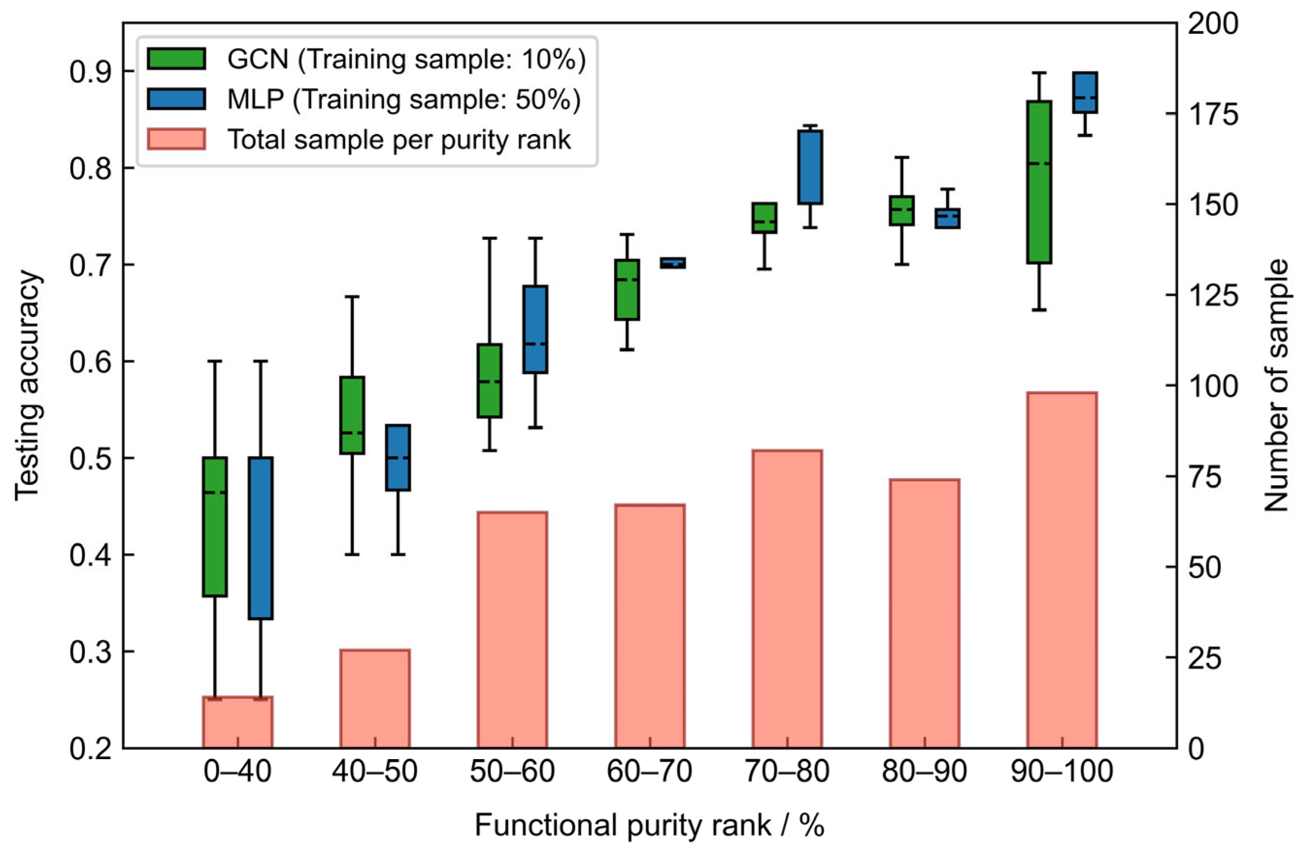
3.1.4. Impact from Different Levels of Functional Heterogeneity

To study the impact of the functional heterogeneity inside areas on the classification accuracy, 5 training sets, each consisting of 10%, are selected out of all samples (using the same stratified sampling method in Section 3.1.3) to train the GCN, and another 5, each consisting of 50% samples, are generated similarly to train the MLP. The occupation percentage of the labeled class (or purity) is calculated for the remaining 90% and 50% samples, based on the same method described in Section 2.1. The purity values are then segmented with an equal interval of 10% to form different purity ranks. The trained models are applied on those samples to observe the relationship between the accuracy and the purity rank. The results are plotted together with a frequency distribution of samples per purity rank in Figure 5.

Results reveal that, whether using 10% or 50% samples (to train GCN and MLP model, respectively), the classification accuracy increases with higher ranking of functional purity, and (or) larger number of samples per purity rank. On the one hand, mixed functions could blur the important features, making it more difficult for the model to distinguish the main function among compound functions. On the other hand, since there is an observed bias in the number of samples of different purities (fewer samples have low purity, as seen in Figure 5), the models may fail to learn enough knowledge to correctly classify low-purity samples. Therefore, we argue that the estimation of functional heterogeneity inside functional areas should be an important procedure in the entire workflow to indicate the confidence of classification results. For example, our experiment in Hong Kong showcases that using road network to divide and generate functional areas, the averaged purity is ~76.1%, and 90.4% samples have higher purity than 50%, meaning a reasonable overall confidence.

3.1.5. Visual Comparison

Figure 6 illustrates the details of urban functional area predictions and the comparisons with the reality maps (derived from the LUHK dataset of Hong Kong following the labeling methods in Section 2.1). In this comparison, to maximize model output differences, the number of training samples is set as 4.7% (known/unknown: 22/469) within the whole region. Images acquired from Sentinel-2A satellite with the spatial resolution of 10 × 10 m is used as a background. Given such a low quantity of training sample, the accuracy ranking from high to low is: GCN (0.68) > MLP (0.63) = RF-128 (0.63) > RF-200 (0.62) > SVM (0.55). As shown in the visual comparison, the GCN exhibits abilities to distinguish functional areas that other models fail to classify correctly. For example, the GCN model effectively identified areas characterized by hospitals and schools (universities) (as indicated by the red boxes, located near Yau Ma Tei area), as well as major business and industrial areas (as indicated by yellow boxes, located at Kwun Tong district). In addition, despite introducing the one-vs.-rest strategy, the SVM classifier failed to distinguish multi-classes within the study area (Figure 6), which may be because it lacks the ability to handle the class imbalance problem introduced in Section 2.3.1.

3.2. Case Study: Beijing

The above analyses have compared and explained model sensitivity (on the training sample size), stability or reproducibility, accuracy, and robustness (from cross validation). Constraints on model applicability are comprehensively studied, which encouraged us to test the classification framework on a very different city in China. Unlike the relatively narrower roads, denser road network and smaller blocks observed in Hong Kong, the urban structure in Beijing is much less affected by terrain factors, but more by anthropological motivations [55,56].

The GCN is outstanding with a small number of training samples, which is important because, in real-world scenarios, lacking training samples of urban functional land use is one of the significant problems, especially in China. Here, for Beijing, the functional land use information of only ~20% of the central urban area (within the 5th ring, ~1140 km²) is known (Figure 7). This small amount of training samples brings challenges and less accuracies if a supervised model (e.g., SVM, RF, MLP) is applied (see Section 3). Thus, the semi-supervised model of graph convolutional network (GCN) is selected in the following urban functional area prediction.

Applications are carried out in parallel for three sub-regions of Beijing to promote the computing efficiency and highlight the heterogeneities within sub-regions. After data processing, 1571 functional areas are generated, with 9.4% (14/149), 8.81% (52/590) and 13.21% (110/833) of the three sub-regions (inside the 2nd ring, 2nd to 4th ring, and outside the 4th ring) selected as training samples. Three sub-regions cover different periods and degrees of development of the city. The 2nd ring encircles the famous Forbidden City and other archaeological landmarks, and outside the 4th ring the area shows less POI data (Figure 7b). Therefore, TF-IDF is calculated on the entire study region scale (within the 5th ring), while the semantic linkage of the cosine similarity is calculated on sub-region scale for highlighting the heterogeneities within sub-regions (see [57,58]).

GCN based classification and validation results are shown in Figure 8. The validation is achieved through field surveys and refers to the online map provided by the Amap platform close to the POI acquisition date. 20/149, 40/590 and 50/833 areas are randomly selected for validation, and the confusion matrixes of each sub-region are derived (Figure 8b). The following results are noticed:

5.

Inside the 2nd ring, commercial, residential, public service, recreational and transportation areas are 51.0%, 8.1%, 35.6%, 4.7% and 0.7% of the related sub-region. From the 2nd to 4th ring, commercial, residential, public service, recreational and transportation areas are 62.7%, 3.1%, 19.7%, 13.9% and 0.7% of the related sub-region. And outside the 4th ring, commercial, residential, public service, recreational and transportation areas are 60.3%, 6.7%, 15.2%, 11.6% and 6% of the related sub-region;

6.

The classification accuracies for three sub-regions are 0.60, 0.83 and 0.69, respectively, and 0.73 for the whole study area. The belt sub-region between the 2nd and 4th ring roads contains a complex distribution of various functional regions, yet exhibits the highest accuracy among three sub-regions. This is in agreement with the relatively high variability observed in the robustness test in Section 3.1.3;

7.

Confusion matrixes indicate relatively higher user accuracies of residential (and recreational) functional land use from 64% to 88% (67% to 100%). The user accuracy of commercial (and public service) functional land use varies in three subareas from 40% to 80% (and 50% to 83%). Transportation functional land use is with less accuracy, which is probably because its low density;

8.

More specifically, public service is located more in the north of the city, while transportation occurs more on the south. On the east side of the 2nd ring, Beijing Central Business District is clearly displaced (the clustered dark red colors). From the 2nd to 4th ring, the well-identified public service areas show the existence of corresponding institutes and universities, especially in the north. To the northwest part of the third sub-region, recreational areas, such as the Summer Palace and Yuanmingyuan, compose distinctive clusters (see the areas colored with dark green). POI point density is relatively low in this region, indicating a lower density of buildings and commercial activities. Areas in the south part of the city are more irregular in shape (Figure 8a), which may be explained by the fact that this region is relatively less planned and developed compared with other regions.

Figure 8. (a) Functional area prediction result within the 5th ring road of Beijing; (b) confusion matrixes of the 3 sub-regions, respectively. The row-normalized matrixes where diagonal element are user accuracies of the corresponding functional land use types.

Figure 8. (a) Functional area prediction result within the 5th ring road of Beijing; (b) confusion matrixes of the 3 sub-regions, respectively. The row-normalized matrixes where diagonal element are user accuracies of the corresponding functional land use types.

4. Discussion

4.1. Sensitivity and Accuracy

The accuracy-efficiency tradeoff: Neural networks are complex architectures and require enormous amounts of training data with good quality to produce viable results. For one neural network, as the size of the training data grows, so does the output accuracies. This is in agreement with [59,60]. However, in choosing different supervised and semi-supervised models, it is not necessarily the more training data the better. An efficient training set size could be selected, according to the cost of the training data and the required output accuracy (Figure 3a). For example, with a 5% training sample, GCN reaches an accuracy of 0.68; with a 40% training sample, RF reaches an accuracy of 0.8; while, with a 80% training sample, MLP reaches an accuracy of 0.85. In this study, the semi-supervised GCN model has better performance in urban functional land use prediction, using only a small number (5%) of training samples, which is meaningful in large-scale, real-world applications.

Reproducibility: Lack of reproducibility in machine learning, which is a complex and growing issue exacerbated by a lack of code transparency, can affect safety, reliability and the detection of bias. In choosing supervised and semi-supervised models, reproducibility comes from two aspects: applying a model multiple times with the same training set (Figure 3a), and a different combination of the same amount of training data (see the cross validation in Figure 4). That is, to obtain a more reliable urban functional land use classification, a model with high reproducibility (less variable in the cross validation) is recommended. In this study, GCN is more stable with the same training set, but varies more in cross-validation with 10% training samples (Figure 4a). MLP is less stable with the same training set, but varies less in cross-validation. And for RF, the increasing of the number of decision tree may not increase the final accuracy, but may increase the model’s instability. This is also reported in previous papers such as [61].

4.2. When Is Machine Learning Application the Best Choice?

As the size of a neural network’s architecture grows, so does its requirement for the amounts of training data. Thus, with a large amount of training samples, model selection and validation would be easy. For example, in modifying present urban functional land use plans with keeping most of the original designs, supervised models such as RF and MLP could be selected. However, there is normally limited training data available in real-world applications. In such cases, supervised classifiers that once have performed well may fail, while exploiting the limited data by incorporating their sematic linkages will produce viable results; see, for example, with 5% training sample, GCN reaches an accuracy of 0.68. This is in agreement with previous research [27], which feeds both feature vectors and different linkages of functional areas (such as the origin and destination pairs of taxi trips) into a GCN model and obtains a lower error. As also implied in previous research [31], the forward and backward training processes of GCN are effectively equivalent to geographical weighted regression (GWR), which makes it suitable in understanding geographical phenomena.

4.3. Limitation and Future Work

Almost always labeled data is essential for machine learning (ML) models. Without enough high-quality labeled data, the use of ML is not recommended. Meanwhile, most ML algorithms work better when there is a spatial balanced or quantitatively equaled distribution for each urban functional area types. In addition, the overfitting problem is noticed when applying MLP over Hong Kong, but in the real application, there may not be enough samples for a validation set to monitor the training process and the overfitting problem. Thus, one should be cautious to apply MLP when there is less than 10% of the whole regions with known classification categories.

In addition to POI data used in this study, other geographical and remote sensing indexes could also improve the classification accuracy [62]. Other similarity methods could also be used to measure the linkage among urban functional areas (see the Moran’s I index and high-resolution image features for example [62,63]). In addition, different segmentation (e.g., OSM based in this study) and different study scale (e.g., sub-regions in Beijing) and urban functional characteristics in neighborhoods, communities, or even regions [37,62], result in varied prediction accuracy. Therefore, each specific method should be considered simultaneously with the available data source, the cost and efficiency for a better outcome. And for future work, within the basic study units, functional characteristics are actually mixed and require more detailed decomposition techniques to better represent the development intensities and interactions in a downscaled situation [27,39]. Furthermore, to deal with the current poor performance diagnosing low-purity samples (Figure 5), new techniques may be needed in the model training process, to specifically improve the ability to discriminate them

5. Conclusions

Formal land use refers to the qualitative attributes of land surface, while functional land use indicates its socioeconomic function. The formal land use map can be created with aerial or remote sensing images, but it is difficult to infer any functional attributes from these observations, especially for urban land use. City planners and other agencies have undertaken surveys to assign or infer the functional characteristics on basic urban areas under their jurisdiction [39]. Such an endeavor is often time-consuming, as the urban landscape is constantly changing with the construction/renovation of infrastructures, new commercial/residential/industrial developments, and the modification of existing uses [20,57,64]. Present geotagged data, e.g., point of interest (POI) data, bring new perspectives in data mining and supplement for defining urban functional area characteristics by associating with machine learning techniques. However, to our knowledge, there are still questions that need to be answered in using present geotagged data to diagnose urban functional areas, such as: When is a machine learning application the best choice? How to select a machine learning model? And what is the model’s uncertainty, robustness and sensitivity?

Therefore, in this study, three supervised (SVM, RF, MLP) and one semi-supervised machine learning model (GCN) are selected. For both supervised and semi-supervised models, a normalized Term Frequency-Inverse Document Frequency (TF-IDF) feature vector for each functional area is calculated as model inputs for the three supervised (SVM, RF, MLP) models. Both the TF-IDF feature vector and the cosine similarity of the TF-IDF feature vectors from two different areas are calculated as model inputs for the semi-supervised GCN model. Followed by the uncertainty, robustness and sensitivity tests (see Section 3), the following results are noticed:

• As the amount of training sample grows, models’ accuracies are improved, but with different potentials. GCN model is with the top accuracy, from 0.65 to 0.70, when the number of training samples is less than 10%, while MLP and RF show top accuracies when the number of training samples exceeds around 10%;
• With a large amount of training samples, which is normally in the modification of existing urban functional area maps, RF and MLP could be the best selection. However, one should note that MLP is less stable with the same training set, but varies less in cross-validation. For RF, the increasing of the number of decision trees may not increase the final accuracy, but may increase the model’s instability;
• With a small amount of training samples, which is normally the case in the real world, GCN could provide viable results by incorporating the auxiliary information provided by the proposed semantic linkages. For example, with the incorporating of the similarity-based semantic linkage, the model could be trained using only 5% of the total samples and produce an accuracy of 0.68;
• In the perspective of the model overfit problem, which could be ignored in the real application due to lacking enough testing samples, when the training samples is less than 10%, we suggest choosing GCN for the urban functional land use prediction, and one should be cautious using MLP, by testing the optimal epoch for obtaining the best accuracy.

References

1. Duranton, G.; Puga, D. Chapter 8—Urban Land Use. In Handbook of Regional and Urban Economics; Duranton, G., Henderson, J.V., Strange, W.C., Eds.; Elsevier: Amsterdam, The Netherlands, 2015; pp. 467–560. [Google Scholar]
2. Cai, D.; Fraedrich, K.; Guan, Y.; Guo, S.; Zhang, C. Urbanization and the thermal environment of Chinese and US-American cities. Sci. Total Environ. 2017, 589, 200–211. [Google Scholar] [CrossRef] [PubMed] [Green Version]
3. Xing, Q.; Sun, Z.; Tao, Y.; Shang, J.; Miao, S.; Xiao, C.; Zheng, C. Projections of future temperature-related cardiovascular mortality under climate change, urbanization and population aging in Beijing, China. Environ. Int. 2022, 163, 107231. [Google Scholar] [CrossRef] [PubMed]
4. Asabere, S.B.; Acheampong, R.A.; Ashiagbor, G.; Beckers, S.C.; Keck, M.; Erasmi, S.; Schanze, J.; Sauer, D. Urbanization, land use transformation and spatio-environmental impacts: Analyses of trends and implications in major metropolitan regions of Ghana. Land Use Policy 2020, 96, 104707. [Google Scholar] [CrossRef]
5. Dadashpoor, H.; Azizi, P.; Moghadasi, M. Land use change, urbanization, and change in landscape pattern in a metropolitan area. Sci. Total Environ. 2019, 655, 707–719. [Google Scholar] [CrossRef] [PubMed]
6. Hu, S.; He, Z.; Wu, L.; Yin, L.; Cui, H. A framework for extracting urban functional regions based on multiprototype word. Computers Environ. Urban Syst. 2019, 80, 101442. [Google Scholar] [CrossRef]
7. Goldstein, J.H.; Caldarone, G.; Duarte, T.K.; Ennaanay, D.; Hannahs, N.; Mendoza, G.; Polasky, S.; Wolny, S.; Daily, G.C. Integrating ecosystem-service tradeoffs into land-use decisions. Proc. Natl. Acad. Sci. USA 2012, 109, 7565–7570. [Google Scholar] [CrossRef] [Green Version]
8. Frias-Martinez, V.; Frias-Martinez, E. Spectral clustering for sensing urban land use using Twitter activity. Eng. Appl. Artif. Intell. 2014, 35, 237–245. [Google Scholar] [CrossRef] [Green Version]
9. Zhai, W.; Bai, X.; Shi, Y.; Han, Y.; Peng, Z.R.; Gu, C. Beyond Word2vec: An approach for urban functional region extraction and identification by combining Place2vec and POIs. Comput. Environ. Urban Syst. 2019, 74, 1–12. [Google Scholar] [CrossRef]
10. Gao, S.; Janowicz, K.; Couclelis, H. Extracting urban functional regions from points of interest and human activities on location-based social networks. Trans. GIS 2017, 21, 446–467. [Google Scholar] [CrossRef]
11. Sanchez, T.W.; Shumway, H.; Gordner, T.; Lim, T. The prospects of artificial intelligence in urban planning. Int. J. Urban Sci. 2022, 1–16. [Google Scholar] [CrossRef]
12. Zhang, J.; He, X.; Yuan, X.-D. Research on the relationship between Urban economic development level and urban spatial structure—A case study of two Chinese cities. PLoS ONE 2020, 15, e0235858. [Google Scholar] [CrossRef] [PubMed]
13. Du, M.; Zhang, X.; Mora, L. Strategic Planning for Smart City Development: Assessing Spatial Inequalities in the Basic Service Provision of Metropolitan Cities. J. Urban Technol. 2021, 28, 115–134. [Google Scholar] [CrossRef]
14. Cariolet, J.-M.; Colombert, M.; Vuillet, M.; Diab, Y. Assessing the resilience of urban areas to traffic-related air pollution: Application in Greater Paris. Sci. Total Environ. 2018, 615, 588–596. [Google Scholar] [CrossRef] [PubMed]
15. Hao, H.; Wang, Y. Disentangling relations between urban form and urban accessibility for resilience to extreme weather and climate events. Landsc. Urban Plan. 2022, 220, 104352. [Google Scholar] [CrossRef]
16. Kim, D.; Song, S.-K. Measuring changes in urban functional capacity for climate resilience: Perspectives from Korea. Futures 2018, 102, 89–103. [Google Scholar] [CrossRef]
17. Ouyang, X.; Wei, X.; Li, Y.; Wang, X.-C.; Klemeš, J.J. Impacts of urban land morphology on PM2. 5 concentration in the urban agglomerations of China. J. Environ. Manag. 2021, 283, 112000. [Google Scholar] [CrossRef]
18. Yu, Z.; Jing, Y.; Yang, G.; Sun, R. A new urban functional zone-based climate zoning system for urban temperature study. Remote Sens. 2021, 13, 251. [Google Scholar] [CrossRef]
19. Yao, Y.; Liu, P.; Hong, Y.; Liang, Z.; Wang, R.; Guan, Q.; Chen, J. Fine-scale intra- and inter-city commercial store site recommendations using knowledge transfer. Trans. GIS 2019, 23, 1029–1047. [Google Scholar] [CrossRef]
20. Klapka, P.; Kraft, S.; Halás, M. Network based definition of functional regions: A graph theory approach for spatial distribution of traffic flows. J. Transp. Geogr. 2020, 88, 102855. [Google Scholar] [CrossRef]
21. Zhao, P.; Luo, A.; Liu, Y.; Xu, J.; Li, Z.; Zhuang, F.; Sheng, V.S.; Zhou, X. Where to Go Next: A Spatio-Temporal Gated Network for Next POI Recommendation. IEEE Trans. Knowl. Data Eng. 2022, 34, 2512–2524. [Google Scholar] [CrossRef]
22. Shen, G.; Zhao, Z.; Kong, X. GCN2CDD: A Commercial District Discovery Framework via Embedding Space Clustering on Graph Convolution Networks. IEEE Trans. Ind. Inform. 2022, 18, 356–364. [Google Scholar] [CrossRef]
23. Yang, J.; Wang, Y.; Xiu, C.; Xiao, X.; Xia, J.; Jin, C. Optimizing local climate zones to mitigate urban heat island effect in human settlements. J. Clean. Prod. 2020, 275, 123767. [Google Scholar] [CrossRef]
24. Lyu, Y.; Wang, M.; Zou, Y.; Wu, C. Mapping trade-offs among urban fringe land use functions to accurately support spatial planning. Sci. Total Environ. 2022, 802, 149915. [Google Scholar] [CrossRef]
25. Guan, Q.; Zhou, J.; Wang, R.; Yao, Y.; Qian, C.; Zhai, Y.; Ren, S. Understanding China’s urban functional patterns at the county scale by using time-series social media data. J. Spat. Sci. 2022, 1–19. [Google Scholar] [CrossRef]
26. Cai, M. Natural language processing for urban research: A systematic review. Heliyon 2021, 7, e06322. [Google Scholar] [CrossRef] [PubMed]
27. Zhu, D.; Zhang, F.; Wang, S.; Wang, Y.; Cheng, X.; Huang, Z.; Liu, Y. Understanding Place Characteristics in Geographic Contexts through Graph Convolutional Neural Networks. Ann. Am. Assoc. of Geogr. 2020, 110, 408–420. [Google Scholar] [CrossRef]
28. Xu, N.; Luo, J.; Wu, T.; Dong, W.; Liu, W.; Zhou, N. Identification and portrait of urban functional zones based on multisource heterogeneous data and ensemble learning. Remote Sens. 2021, 13, 373. [Google Scholar] [CrossRef]
29. Zhang, W.; Liu, H.; Liu, Y.; Zhou, J.; Xu, T.; Xiong, H. Semi-Supervised City-Wide Parking Availability Prediction via Hierarchical Recurrent Graph Neural Network. IEEE Trans. Knowl. Data Eng. 2022, 34, 3984–3996. [Google Scholar] [CrossRef]
30. Kim, N.; Yoon, Y. Effective Urban Region Representation Learning Using Heterogeneous Urban Graph Attention Network (HUGAT). arXiv preprint 2022, arXiv:2202.09021. [Google Scholar]
31. Zhu, D.; Liu, Y.; Yao, X.; Fischer, M.M. Spatial regression graph convolutional neural networks: A deep learning paradigm for spatial multivariate distributions. GeoInformatica 2022, 26, 645–676. [Google Scholar] [CrossRef]
32. Geng, X.; Li, Y.; Wang, L.; Zhang, L.; Yang, Q.; Ye, J.; Liu, Y. Spatiotemporal Multi-Graph Convolution Network for Ride-Hailing Demand Forecasting. Proc. AAAI Conf. Artif. Intell. 2019, 33, 3656–3663. [Google Scholar] [CrossRef]
33. Chi, J.; Jiao, L.; Dong, T.; Gu, Y.; Ma, Y. Quantitative identification and visualization of urban functional area based on POI data. J. Geomat 2016, 41, 68–73. [Google Scholar]
34. Miao, R.; Wang, Y.; Li, S. Analyzing urban spatial patterns and functional zones using sina Weibo POI data: A case study of Beijing. Sustainability 2021, 13, 647. [Google Scholar] [CrossRef]
35. Li, Y.; Liu, C.; Li, Y. Identification of Urban Functional Areas and Their Mixing Degree Using Point of Interest Analyses. Land 2022, 11, 996. [Google Scholar] [CrossRef]
36. Zhang, X.; Du, S.; Wang, Q. Hierarchical semantic cognition for urban functional zones with VHR satellite images and POI data. ISPRS J. Photogramm. Remote Sens. 2017, 132, 170–184. [Google Scholar] [CrossRef]
37. Zhan, X.; Ukkusuri, S.V.; Zhu, F. Inferring Urban Land Use Using Large-Scale Social Media Check-in Data. Netw. Spat. Econ. 2014, 14, 647–667. [Google Scholar] [CrossRef]
38. Wong, K.S.; Tanaka, K. Data embedding for geo-tagging any contents in smart device. In Proceedings of the 2014 IEEE Region 10 Symposium, Kuala Lumpur, Malaysia, 14–16 April 2014. [Google Scholar]
39. Hu, Y.; Han, Y. Identification of Urban Functional Areas Based on POI Data: A Case Study of the Guangzhou Economic and Technological Development Zone. Sustainability 2019, 11, 1385. [Google Scholar] [CrossRef] [Green Version]
40. Iranmanesh, A.; Cömert, N.Z.; Hoşkara, Ş.Ö. Reading urban land use through spatio-temporal and content analysis of geotagged Twitter data. GeoJournal 2022, 87, 2593–2610. [Google Scholar] [CrossRef]
41. Kipf, T.; Welling, M. Semi-Supervised Classification with Graph Convolutional Networks. arXiv 2016, arXiv:1609.02907. [Google Scholar]
42. Yuan, J.; Zheng, Y.; Xie, X. Discovering regions of different functions in a city using human mobility and POIs. In Proceedings of the 18th ACM SIGKDD international conference on Knowledge discovery and data mining 2012, Association for Computing Machinery, Beijing, China, 12–16 August 2012; pp. 186–194. [Google Scholar]
43. Liu, W.; Lü, L. Link prediction based on local random walk. EPL (Europhys. Lett.) 2010, 89, 58007. [Google Scholar] [CrossRef] [Green Version]
44. Cortes, C.; Vapnik, V. Support-vector networks. Mach. Learn. 1995, 20, 273–297. [Google Scholar] [CrossRef]
45. Breiman, L. Random forests. Mach. Learn. 2001, 45, 5–32. [Google Scholar] [CrossRef] [Green Version]
46. Saravanan, R.; Sujatha, P. A State of Art Techniques on Machine Learning Algorithms: A Perspective of Supervised Learning Approaches in Data Classification. In Proceedings of the 2018 Second International Conference on Intelligent Computing and Control Systems (ICICCS), Madurai, India, 14–15 June 2018. [Google Scholar]
47. Aly, M. Survey on multiclass classification methods. Neural Netw 2005, 19, 9. [Google Scholar]
48. Lin, T.Y.; Goyal, P.; Girshick, R.; He, K.; Dollár, P. Focal Loss for Dense Object Detection. IEEE Trans. Pattern Anal. Mach. Intell. 2017, 99, 2999–3007. [Google Scholar]
49. Woldesemayat, E.M.; Genovese, P.V. Urban Green Space Composition and Configuration in Functional Land Use Areas in Addis Ababa, Ethiopia, and Their Relationship with Urban Form. Land 2021, 10, 85. [Google Scholar] [CrossRef]
50. Junker, M.; Hoch, R.; Dengel, A. On the evaluation of document analysis components by recall, precision, and accuracy. In Proceedings of the Fifth International Conference on Document Analysis and Recognition ICDAR’99 (Cat. No. PR00318), Bangalore, India, 22 September 1999. [Google Scholar]
51. Dietterich, T. Overfitting and undercomputing in machine learning. ACM Comput. Surv. (CSUR) 1995, 27, 326–327. [Google Scholar] [CrossRef]
52. Parsons, V.L. Stratified sampling. Wiley StatsRef Stat. Ref. Online 2014, 1–11. [Google Scholar]
53. Stone, M. Cross-validation:a review. Ser. Stat. 1978, 9, 127–139. [Google Scholar] [CrossRef]
54. Xu, K.; Hu, W.; Leskovec, J.; Jegelka, S. How Powerful are Graph Neural Networks? ArXiv 2019, arXiv:1810.00826. [Google Scholar]
55. Ganesan, S.; Lau, S.S.Y. Urban challenges in Hong Kong: Future directions for design. Urban Des. Int. 2000, 5, 3–12. [Google Scholar] [CrossRef]
56. Liu, G.; Yang, Z.; Chen, B.; Ulgiati, S. Monitoring trends of urban development and environmental impact of Beijing, 1999–2006. Sci. Total Environ. 2011, 409, 3295–3308. [Google Scholar] [CrossRef] [PubMed]
57. Zhang, X.; Du, S. A Linear Dirichlet Mixture Model for decomposing scenes: Application to analyzing urban functional zonings. Remote Sens. Environ. 2015, 169, 37–49. [Google Scholar] [CrossRef]
58. Wang, J.-F.; Zhang, T.-L.; Fu, B.-J. A measure of spatial stratified heterogeneity. Ecol. Indic. 2016, 67, 250–256. [Google Scholar] [CrossRef]
59. van Engelen, J.E.; Hoos, H.H. A survey on semi-supervised learning. Mach. Learn. 2020, 109, 373–440. [Google Scholar] [CrossRef] [Green Version]
60. Li, C.; Wang, J.; Wang, L.; Hu, L.; Gong, P. Comparison of Classification Algorithms and Training Sample Sizes in Urban Land Classification with Landsat Thematic Mapper Imagery. Remote Sens. 2014, 6, 964–983. [Google Scholar] [CrossRef] [Green Version]
61. Jin, H.; Stehman, S.V.; Mountrakis, G. Assessing the impact of training sample selection on accuracy of an urban classification: A case study in Denver, Colorado. Int. J. Remote Sens. 2014, 35, 2067–2081. [Google Scholar] [CrossRef]
62. Zhang, K.; Ming, D.; Du, S.; Xu, L.; Ling, X.; Zeng, B.; Lv, X. Distance Weight-Graph Attention Model-Based High-Resolution Remote Sensing Urban Functional Zone Identification. IEEE Trans. Geosci. Remote Sens. 2022, 60, 1–18. [Google Scholar] [CrossRef]
63. Wu, Y.; Zhuang, D.; Labbe, A.; Sun, L. Inductive Graph Neural Networks for Spatiotemporal Kriging. Proc. AAAI Conf. Artif. Intell. 2021, 35, 4478–4485. [Google Scholar] [CrossRef]
64. Wang, Y.; Wang, T.; Tsou, M.-H.; Li, H.; Jiang, W.; Guo, F. Mapping Dynamic Urban Land Use Patterns with Crowdsourced Geo-Tagged Social Media (Sina-Weibo) and Commercial Points of Interest Collections in Beijing, China. Sustainability 2016, 8, 1202. [Google Scholar] [CrossRef]
Figure 1. A flowchart illustrating the five stages of the functional area type identification and classification conducted in this paper.
Remotesensing 15 00341 g001
Figure 2. (a) Geographical setting of the study region, Hong Kong, China. The research is carried out within the red lines; (b) histogram statistics of the size for the functional area; (c) kernel density distribution of Point of Interest (POI) points; and (d) the functional land use distribution derived from the dataset of Land Utilization in Hong Kong (LUHK), including five categories: commercial, residential, public service, recreational and transportation.
Remotesensing 15 00341 g002
Figure 3. (a) Comparing training set size dependence associated with five functional area classification models: support vector machine (SVM), random forest (RF-128 and RF-200), multi-layer perceptron (MLP) and graph convolutional network (GCN), indicating a best performance with GCN under semi-supervised situation and a best performance with MLP under supervised situation; (b) and (c) the testing accuracy and testing loss curves for MLP and GCN during model trainings.
Remotesensing 15 00341 g003
Figure 5. The correlation between accuracy and different functional purities with the frequency distribution of purity ranks.
Remotesensing 15 00341 g005
Figure 6. Visual comparison between ground truth and five functional land use prediction results obtained from SVM, RF-128, RF-200, MLP and GCN. The number of training samples is set as 4.7% (known/unknown: 22/469) of the total region, and the accuracy is highlighted accordingly.
Remotesensing 15 00341 g006
Figure 7. (a) Geographical setting of the study region, Beijing, China. The research is carried out within the 5th ring road (marked by the red line); (b) histogram statistics of the size for the functional area; (c) kernel density distribution of local point of interest (POI) points; and (d) the functional land use distribution obtained from the open street map land use dataset, including five categories: commercial, residential, public service, recreational and transportation.
Remotesensing 15 00341 g007