Multi-Level Fusion Indoor Positioning Technology Considering Credible Evaluation Analysis

Abstract

Aiming at the problems of the low robustness and poor reliability of a single positioning source in complex indoor environments, a multi-level fusion indoor positioning technology considering credible evaluation is proposed. A multi-dimensional electromagnetic atlas including pseudolites (PL), Wi-Fi and a geomagnetic field is constructed, and the unsupervised learning model is used to sample in the latent space to achieve a feature-level fusion positioning. A location credibility evaluation method is designed to improve the credibility of the positioning system through a multi-dimensional data quality evaluation and heterogeneous information auxiliary constraints. Finally, a large number of experiments were carried out in the laboratory environment, and, finally, about 90% of the positioning error was better than 1 m, and the average positioning error was 0.56 m. Compared with several relatively advanced positioning methods (Inter-satellite CPDM/Epoch-CPDS/Z-KPI) at present, the average positioning accuracy is improved by about 56%, 83.5% and 82.9%, respectively, which verifies the effectiveness of the algorithm. To verify the effect of the proposed method in a practical application environment, the proposed positioning system is deployed in the 2022 Winter Olympics venues. The results show that the proposed method has a significant improvement in the positioning accuracy and continuity.

1. Introduction

Location information is the basis for the development of a digital and intelligent society, an important part of the Internet of Everything, and has been fully penetrated into human daily life. Global navigation satellite system (GNSS) application fields are almost ubiquitous, including air, sea, ground and rail transportation and management, smart grids, telecommunication systems and financial systems, smartphone positioning and location services, autonomous driving and other scenarios. The birth of the GNSS is revolutionizing the world’s politics, military, technology, culture and many other aspects [1,2]. However, the common focus of industry and academia, the PNT (positioning, navigation and timing) technology in the GNSS signal denial environment, has not been solved, especially the indoor positioning technology in the PNT, which has not been able to achieve a fundamental breakthrough. Generally, indoor positioning technology includes active positioning means and passive positioning means [3,4]. Among them, active positioning needs to rely on infrastructure base stations and wireless access points in the environment, such as Wi-Fi [5,6,7], UWB (ultra-wideband) [8,9,10], sound [11,12,13], Bluetooth [14,15,16], etc., usually using localization methods such as TOA (time of arrival) [17,18], TDOA (time difference of arrival) [19], TOF (time of flight) [20], AOA (angle of arrival) [21] and fingerprint matching [22]. Passive positioning usually refers to the positioning system based on the target’s own sensors, such as the inertial sensor-based pedestrian dead reckoning (PDR) to achieve the target’s position recursion [23], which includes heading estimation [24], step state detection [25] and step estimation [26].

Although there are many types of indoor positioning technologies, in harsh indoor environments such as multi-occlusion, strong interference, rich multi-path and non-LOS, a single positioning signal or positioning feature often inevitably leads to information loss, errors and other unreliable information phenomena. This will make it difficult to meet the continuous and stable indoor high-precision positioning requirements only by relying on certain positioning feature information. Multi-source information fusion positioning technology can fuse a variety of positioning feature information to overcome the problem when the system cannot be positioned normally due to problems such as information loss, environmental interference and signal transmission delay. Therefore, it is necessary to combine other positioning source information to improve the stability and practicability of the system. Based on the above ideas, this paper designs a multi-dimensional atlas fusion positioning technology based on pseudolites, Wi-Fi and a geomagnetic field. Among them, pseudolites have the advantage of being highly compatible with GNSS navigation satellites, enabling continuous indoor and outdoor positioning based on the same user terminal, and gradually become an important signal source in the field of indoor positioning [27]. For example, a positioning method based on pseudolite fingerprints proposed in [27] can effectively solve the positioning problem in non-LOS environments, but only uses a single data source information and cannot deal with problems such as signal loss. In the literature [28,29], the method based on a carrier difference search and the method of a Doppler frequency shift velocity measurement were designed, both of which achieved sub-meter positioning accuracy, but did not consider the influence of signal non-LOS.

In response to the above problems, this paper integrates the most common Wi-Fi signals in indoor buildings and zero-cost geomagnetic field information to achieve a lightweight, high-precision and stable indoor positioning solution as much as possible. In terms of the fusion method, a feature extraction model based on a CNN network-assisted variational autoencoder is designed, drawing on the advantages of deep learning in feature extraction. Among them, CNN is used to extract the inter-pixel features of the multi-dimensional electromagnetic atlas, and the autoencoder is used to learn the distribution of the feature space. Combined with noise reduction processing, the anti-interference of the positioning system is improved. The specific contributions are as follows:

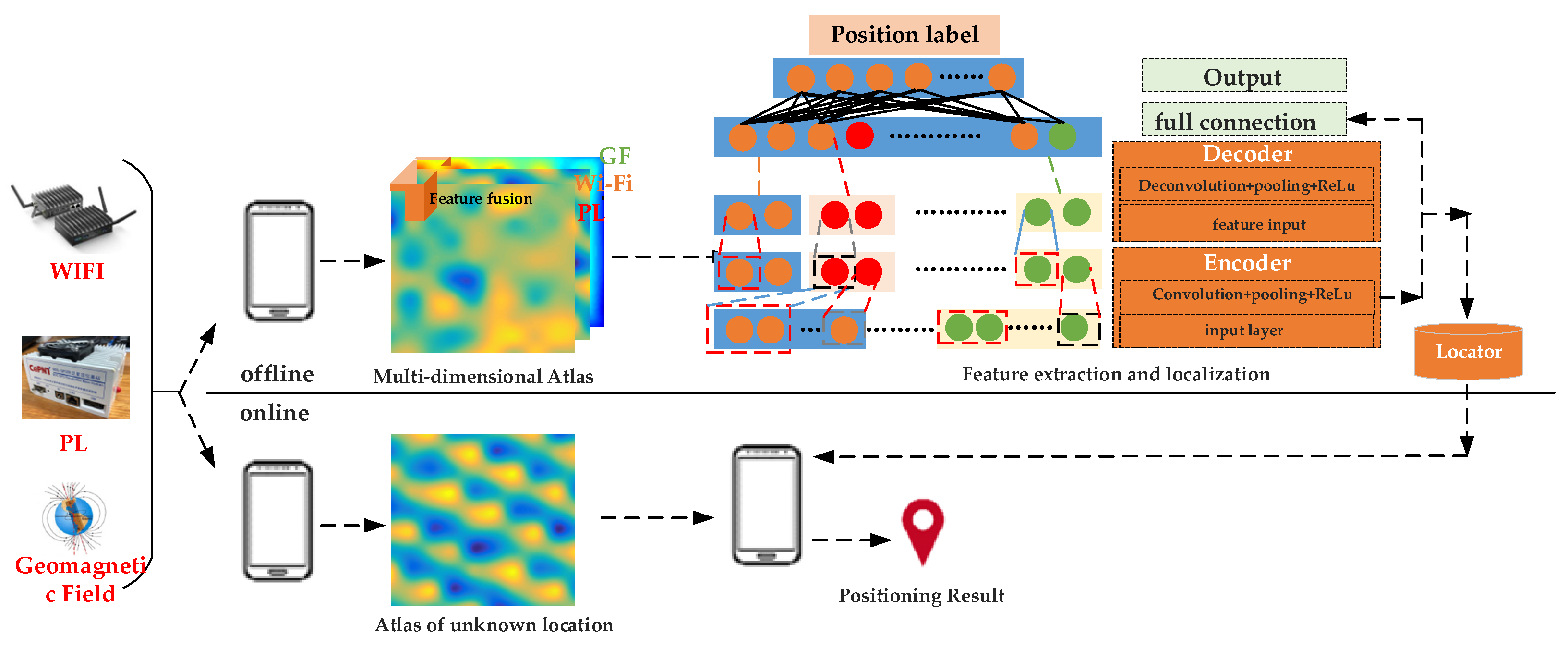
• Aiming at the problems of a single data type and poor robustness in traditional localization, a multi-dimensional feature fusion localization method based on deep learning is proposed. A deep convolutional neural network-assisted denoising variational autoencoder (DVAE-CNN) localization model is designed. The latent feature extraction and fusion are carried out on the multi-dimensional electromagnetic signal map including pseudolite, Wi-Fi and geomagnetic information in the indoor environment. Finally, by establishing the mapping relationship between the multi-dimensional deep features and the spatial position, the absolute position estimation of the target in the indoor environment is realized.
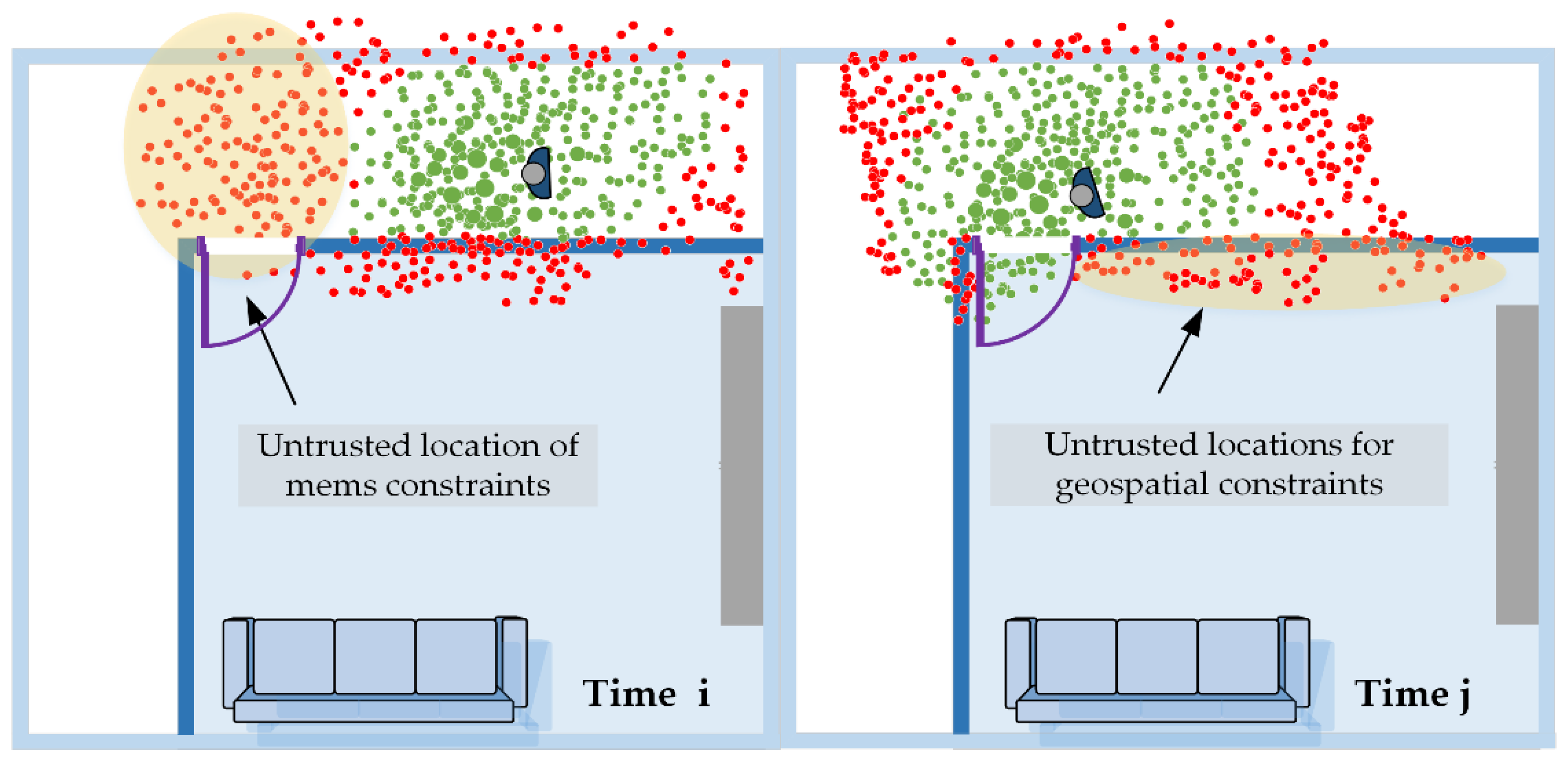
• Aiming at the problems of the poor continuity and low reliability of positioning results caused by the occlusion and interference of indoor positioning signals, a credible evaluation and analysis method based on the combination of an unsupervised autoencoder and particle filter is proposed. The multi-source heterogeneous data quality evaluation model, geographic prior information and MEMS sensor information are effectively integrated, and the positioning performance is improved by constraining the particle state transition equation and weight update method.
• In order to verify the performance of the positioning method, a large number of experiments were carried out in the test field environmen. Finally, the effectiveness of the proposed multi-level fusion positioning’s trusted positioning was verified, and a high-precision positioning better than 1 m (90%) was achieved. At the same time, the proposed method was successfully applied to the large stadiums of the 2022 Beijing Winter Olympics, providing continuous high-precision location services for security, epidemic prevention and other operation teams, and promoting the development of indoor positioning industrialization.

The rest of this paper is organized as follows: In the second part, the work related to this research content is introduced, and the indoor pseudolites, Wi-Fi and geomagnetic distribution characteristics are comprehensively analyzed. The proposed positioning technology framework and workflow are described in Section 3. The fusion details of the deep learning-based indoor localization techniques are introduced in Section 4. In Section 5, the localization performance of the proposed method is verified through extensive experiments. In the last section, the article is summarized, and the strengths and limitations of the method are discussed, as well as some future work to be undertaken.

2. Related Work

The positioning method based on fingerprint feature matching is not easily interfered with by factors such as multipath and non-LOS, so it has become one of the commonly used positioning techniques. However, in the fingerprint matching positioning theory, the positioning error will be affected by environmental changes. Generally speaking, it mainly comes from the representation of the feature and the position ambiguity problem.

In the first aspect, the characterization method of features is mainly reflected in the structure of features and the calculation method of feature similarity [30]. Different fingerprint feature composition methods and different feature similarity calculation methods will affect the performance of the matching and positioning. For example, in reference [31], the authors analyzed the long-term variation of fingerprint data in detail. At the same time, 3D positioning is achieved through higher fine-grained data features combined with Bayesian inference. In addition, a method for the distance prediction of a received signal indicator (RSSI) in a complex indoor environment is proposed in [32]. The technology of the transceiver height and Fresnel ranging is considered to better adapt to the path loss of the RSSI. From the perspective of signal characteristic transmission, it is helpful to improve the indoor positioning performance. The spatial discrimination of the feature is an important indicator to measure the performance of the characterization method of the feature. The higher the spatial discrimination of the feature, the higher the resolution in the physical space, and the higher the accuracy that can be obtained when it is used for positioning. Therefore, the feature discrimination is one of the main sources of errors in the fingerprint identification system. On the other hand, the problem of location ambiguity that different locations exhibit similar feature fingerprints is also a source of error [32]. Typically, local ambiguity occurs when similar signals appear at close positions, but is susceptible to local blurring, whereas magnetic field fingerprints are the opposite. Another example is that the fingerprint data of the pseudolite carrier phase have the problem of ambiguity and an ambiguous area of positioning, but the local area has a high spatial resolution, which can achieve higher-precision positioning. Therefore, in complex positioning scenarios, it is difficult to obtain a high spatial discrimination degree only by a certain positioning feature. In this case, using multi-source information to characterize fingerprint features is a powerful means to improve the spatial discrimination degree of features. However, the current feature characterization methods mostly use feature combination, and the similarity calculation model of features is relatively fixed, so this restricts the improvement of the spatial discrimination of features. Therefore, the spatial distribution characteristics of the electromagnetic field in the indoor space environment are analyzed in detail, and the specific analysis is as follows.

(1) PL carrier phase difference data are a stable and reliable fingerprint information, which can characterize the moving direction and environmental occlusion of the target. As shown in Figure 1, the two-dimensional distribution of the carrier phase difference (CPD) between the multiple signals of the homologous array pseudolite is plotted in the physical space, and the horizontal and vertical coordinates are the dimensions of the analysis area (unit: m). Not hard to find, when the positioning area increases, there are more ambiguous areas in the pseudolite carrier phase, resulting in a larger positioning error. In addition, there are differences in the number of pseudolites received in different regions, and the quality of the received signals will also be interfered with by the environment. Therefore, it is difficult to achieve large-scale and stable high-precision positioning only by using pseudolite data as fingerprints.

(2) The Wi-Fi wireless network gradually covers most of the indoor areas. Using the existing Wi-Fi infrastructure for positioning is a low-cost and lightweight solution. Traditional RSS fingerprinting is one of the most popular positioning methods. Usually, Wi-Fi RSS data are used to build a radio map, and online real-time matching is used to obtain a rough location. Figure 2 shows the signal strength distribution of the four APs (access points) in the test area, which can generally be used to distinguish geographic locations. However, it will lead to large localization errors due to low spatial resolution.

(3) The ubiquitous geo-magnetic field is a potential indoor positioning technology that does not depend on infrastructure. There are several ways to locate it using geomagnetic information. One is to use magnetic field information to calculate the heading, which is usually used in a PDR algorithm. However, it is easy to be affected by building materials, and the estimation accuracy is not high. On the contrary, another method is to use the magnetic field anomaly as a unique feature to distinguish different indoor areas or indoor and outdoor areas, and its advantages are low cost and low energy consumption. However, the degree of discrimination of geomagnetic signals is limited, and it is difficult to achieve high-precision indoor positioning. It is experimentally confirmed in [33] that the influence of moving objects is very limited, with almost no influence at a distance of one meter. Moreover, although there are differences in the data collected by different devices and different device orientations, the shape of the data curve on the same path is the same, so the method of subtracting the mean is usually used for preprocessing to achieve data standardization. As shown in Figure 3, the spatial distribution differences of the X, Y, Z axes and modulus of the geomagnetic field are plotted, which shows that it has a certain ability to distinguish locations.

Based on the above analysis, the length and width of the picture represent the length and width of the test geographic area, respectively, and the color depth represents the signal space difference. The three types of information are collected in the same area, and the spatial resolution scale (signal variation range/geospatial size) has a higher big difference. Therefore, the fundamental reason why pseudolite signals, Wi-Fi and geomagnetic information can be fused lies in their complementary position resolution capabilities. Conceptually, the navigation signal and Wi-Fi are a kind of radio, and the signal transmission distance is affected by the distance. For example, the area with a long distance will lead to a weak signal strength or even loss of signal lock, and the coverage is limited. The geomagnetic field is global navigation information, and the distribution of the magnetic field is related to the built environment, which is unique to the scene. Therefore, combining the three will be able to achieve a higher resolution and wider coverage positioning capabilities.

3. Method

The technical route of the proposed algorithm is shown in Figure 4. The realization of the positioning algorithm includes two parts: the offline stage and the online stage. The offline stage includes the acquisition and processing of multi-dimensional electromagnetic data, as well as the construction and training of feature models and locators, and then packaged into lightweight models that can be used in engineering applications. The online stage includes two parts: calling the model and real-time positioning. The credible evaluation model, the locator model, the MEMS sensor information and the prior geographic information are fused through the particle filter algorithm to achieve rapid positioning in the indoor building environment.

3.1. Multi-Dimensional Electromagnetic Atlas Fusion Positioning Technology

In this section, a localization method based on a multi-dimensional electromagnetic atlas is proposed. By building a deep learning localization model, the feature extraction and analysis of the multi-source hybrid map composed of multi-source heterogeneous radio signals and geomagnetic field signals in the structured space environment are carried out. A mapping model of electromagnetic signals and location information in indoor space is established to achieve target tracking and positioning.

A VAE (variational autoencoder) is an unsupervised generative model that encodes based on a Gaussian mixture model. Simply put, any distribution can be decomposed into the superposition of several Gaussian distributions, and a VAE is used to describe the hidden variables from the perspective of probability. By extracting the data features, the distribution characteristics of the pseudo satellite, indoor Wi-Fi and geomagnetic information at different locations are abstracted, and the feature clustering of the multi-dimensional fingerprint data in the indoor environment under the hidden space are realized. Then, the learned latent features are used as an input to train the localization model. The respective distributions of the pseudolite observation data, Wi-Fi data and geomagnetic data received at any location in the indoor area can be regarded as the accumulation of the signal distributions in the integral domain. However, the process of solving the signal distribution based on basic mathematical methods is usually complicated, so this paper uses a VAE to encode the multi-dimensional input data. By extracting the latent features, the original messy fingerprint data are clustered in the two-dimensional latent space, and the regular representative deep features are obtained. Among them, the output of the model is the mean and variance of each group of data, so the latent characteristics can be regarded as a continuous distribution, and different coding results are obtained by sampling each time. Therefore, the non-linear transformation process will not cause too large a migration deviation between points at the time of encoding, which improves the error tolerance of the decoder. Since the multi-dimensional electromagnetic atlas constructed in this paper can be regarded as a multi-dimensional color image, the multi-dimensional atlas is processed by multi-layer convolution in the encoding and decoding stage by drawing on the advantages of the CNN in processing images. The purpose of noise reduction is to solve the problem that each signal source in different indoor areas may lose lock, resulting in an inconsistent number of signals collected in different areas. The basic principle block diagram of the positioning technology is shown in Figure 5.

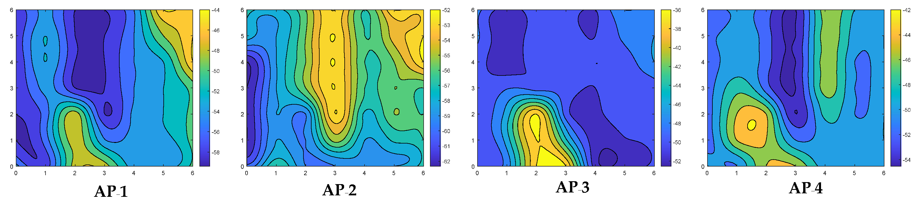
3.1.1. Information Collection and Electromagnetic Atlas Construction

Usually, the traditional fingerprint database construction is a time-consuming and labor-intensive work, which makes it difficult to popularize and apply. In order to improve the efficiency of the data collection and construction of an offline multi-dimensional atlas, a dynamic database construction device combining foot inertial navigation, multi-sensor receivers and smart phones is designed. The smartphone is mainly used for IMU initialization and error calibration, data collection and real-time data observation, and each part transmits data through Bluetooth. In the offline construction stage, the zero-speed correction method is used to eliminate the accumulated error of the foot inertial navigation to obtain relatively accurate position coordinates, which are used to mark the multi-dimensional atlas data. Here, the initial sensor calibration, Bluetooth connection, data acquisition, data storage and data upload are completed based on the self-developed acquisition software, as shown in Figure 6. In addition, the geodetic latitude and longitude coordinate system and the Gauss plane Cartesian coordinate system are used in this paper. Among them, the former is used for the space reference of the inertial measurement unit, and the latter is used for the reference frame of the final output of the positioning system, and the two are unified through conversion.

In data acquisition, since the inertial unit will generate accumulated errors for a long time, the acquisition personnel will measure multiple calibration points with real coordinates in advance in the environment. According to the positioning accuracy requirements, when the deviation between the inertial navigation output result and the calibration point position exceeds a certain range, the tester clicks the position calibration button, thereby improving the accuracy of the dataset construction.

Due to the different data types and dimensions of the collected data, it is impossible to directly construct and integrate the dataset. Therefore, the multi-dimensional heterogeneous data need to be standardized and used for the training of the positioning model. For different types of positioning data sources, the regularized data are obtained by preprocessing separately and then forming a new feature space for feature matching and positioning.

As can be seen from Figure 7, the multi-dimensional atlas information includes the inter-satellite carrier phase difference of multi-channel pseudolites, where n is the number of pseudolites channels and m is the number of Wi-Fi. Through data preprocessing, various types of data are fused to form a multi-dimensional electromagnetic atlas.

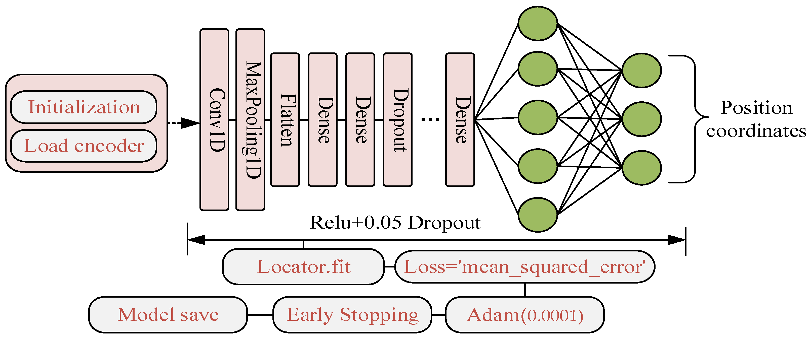
3.1.2. Positioning Model Construction and Training

In the previous section, the construction of a multi-dimensional electromagnetic atlas was completed, and various data were stacked together in the form of characteristic images. For such a dataset, a convolutional neural network-assisted denoising variational autoencoder network (DVAE-CNN) is designed.

Generally speaking, an autoencoder consists of two parts: an encoder and a decoder. The encoder maps data X to a hidden layer h, where h is the latent representation of the data. Similarly, the DVAE is also expressing and using features after mapping the original data with noise to the hidden feature space. Its purpose is to allow the encoder encoding to have some small errors when predicting the hidden variable z, and still be able to accurately represent the input data X. The goal of the DVAE is to learn the parameter $\theta$, so as to maximize the edge probability density function $p_{\theta }\left(x\right)={\displaystyle \int p_{{}_{\theta }}\left(x|z\right)}{p}_{\theta }\left(z\right)dz$, and realize the ability to recover the original data by using the features extracted from the noise data. It is usually difficult to deal with the posterior probability $p_{\theta }\left(z|\tilde{x}\right)$ and $p\left(\tilde{x},z\right)=p\left(\tilde{x}\right)p\left(z|\tilde{x}\right)$, so it is necessary to use $q_{\varphi }\left(z|\tilde{x}\right)$ to approximate. Then, we can use the joint distribution $q_{\varphi }\left(\tilde{x},z\right)$ to approximate the $p_{\theta }\left(\tilde{x},z\right)$, and then to calculate the KL (Kullback–Leibler divergence) [34] of the two distributions to calculate the similarity, there is:

$$KL\left(p_{\theta }\left(\tilde{x},z\right)\Vert q_{\varphi }\left(\tilde{x},z\right)\right)={\displaystyle \iint p_{\theta }\left(\tilde{x},z\right)\log \frac{p_{\theta }\left(\tilde{x},z\right)}{q_{\varphi }\left(\tilde{x},z\right)}}dzdx$$

(1)

The KL divergence is optimized so that the two distributions are as close as possible. Among them, the latent variable $z$ is constrained by resampling [34], so that the hidden feature z can represent the characteristics of the noise observation data x, so there are:

$$KL\left(p_{\theta }\left(\tilde{x},z\right)\Vert q_{\varphi }\left(\tilde{x},z\right)\right)={\mathrm{E}}_{x\sim p_{\theta }\left(\tilde{x}\right)}\left[{\displaystyle \int p_{\theta }\left(z|\tilde{x}\right)\log \frac{p_{\theta }\left(\tilde{x}\right)p_{\theta }\left(z|\tilde{x}\right)}{q_{\varphi }\left(\tilde{x},z\right)}dz}\right]$$

(2)

Since $\log \frac{p_{\theta }\left(\tilde{x}\right)p_{\theta }\left(z|\tilde{x}\right)}{q_{\varphi }\left(\tilde{x},z\right)}=\log p_{\theta }\left(\tilde{x}\right)+\log \frac{p_{\theta }\left(z|\tilde{x}\right)}{q_{\varphi }\left(\tilde{x},z\right)}$, Equation (2) can be simplified as:

$$KL\left(p_{\theta }\left(x,z\right)\Vert q_{\varphi }\left(\tilde{x},z\right)\right)={\mathrm{E}}_{x\sim p_{\theta }\left(\tilde{x}\right)}\left[\log p_{\theta }\left(\tilde{x}\right)\right]+{\mathrm{E}}_{x\sim p_{\theta }\left(\tilde{x}\right)}\left[{\displaystyle \int p_{\theta }\left(z|\tilde{x}\right)\log \frac{p_{\theta }\left(z|\tilde{x}\right)}{q_{\varphi }\left(\tilde{x},z\right)}dz}\right]$$

(3)

Then, because of $KL\left(p_{\theta }\left(\tilde{x},z\right)\Vert q_{\varphi }\left(\tilde{x},z\right)\right)\ge 0$ and $q_{\varphi }\left(\tilde{x},z\right)=q_{\varphi }\left(\tilde{x}|z\right)q_{\varphi }\left(z\right)$, so

$$\log p_{\theta }\left(\tilde{x}\right)\ge -\left[{\displaystyle \int p_{\theta }\left(z|\tilde{x}\right)\log \frac{p_{\theta }\left(z|\tilde{x}\right)}{q_{\varphi }\left(x|z\right)q_{\varphi }\left(z\right)}dz}\right]$$

(4)

Among them, $-\left[{\displaystyle \int p_{\theta }\left(z|\tilde{x}\right)\log \frac{p_{\theta }\left(z|\tilde{x}\right)}{q_{\varphi }\left(x|z\right)q_{\varphi }\left(z\right)}dz}\right]$ is the lower limit (ELBO, evidence lower bound objective) of the function. At this time, only the ELBO needs to be constrained, so there are:

$$ELBO\left(\theta ,\varphi ,\tilde{x}\right)=-KL\left(p_{\theta }\left(z|\tilde{x}\right)\Vert q_{\varphi }\left(z\right)\right)+{\mathrm{E}}_{z\sim p_{\theta }\left(z|\tilde{x}\right)}\left[\log q_{\varphi }\left(x|z\right)\right]$$

(5)

In the above Equation (5), the latent variable $z$ is usually regarded as a standard normal distribution, which can effectively prevent the variational encoder from degenerating to AE after processing.

$p_{\theta }\left(z|\tilde{x}\right)\sim N\left(\mu \left(\tilde{x}\right),{\sigma }^2\left(\tilde{x}\right)\right)$, the distribution can be fitted by building a neural network, $\tilde{x}$ is the input data, the mean is $\mu \left(\tilde{x}\right)$ and the variance is ${\sigma }^2\left(\tilde{x}\right)$ as the output of the neural network, where $\varphi$ and $\theta$ are the parameters of the encoder and decoder, respectively, and the second term on the right side of the equation represents the reconstruction error as $E_p\left(\log q\right)$, so Equation (5) can be written as:

$$-KL\left(p_{\theta }\left(z|\tilde{x}\right)\Vert q_{\varphi }\left(z\right)\right)=\frac{1}{2}{\displaystyle \sum _{m=1}^M\left(1+\log {\left({\sigma }_m\right)}^2-{\left({\mu }_m\right)}^2-{\left({\sigma }_m\right)}^2\right)}$$

(6)

where $m$ is the $m$-th dimension of the latent variable z, M is the dimension of the latent variable and ${\mu }_m$ and ${\sigma }_m$ represent the m-th variable of the mean and variance of the general normal distribution $p_{\theta }\left(z|\tilde{x}\right)$, respectively.

The above content describes the basic process of a VAE model feature extraction, which can model the distribution of radio signals in the indoor space environment, which greatly improves the performance of the indoor positioning of wireless signals. Since three different types of data are imaged in this paper, the data input to the VAE network is actually a multi-dimensional image. Therefore, this paper chooses to use the convolutional neural network, CNN, to process the feature extraction. Based on the multi-layer convolution operation, the correlation between image pixels can be learned, thereby improving the generalization ability of the model. Combining the CNN with other methods helps the network to excel in spatial relationships. At the same time, the convolutional layer is an important part of the deep neural network, combined with the powerful generative model capability of the autoencoder. It helps to reconstruct its output through deep feature recognition as well as high-fidelity encoding. The basic framework is to use several convolutional layers for feature extraction in the encoder, and a corresponding deconvolutional layer to mirror the network in the decoder.

Specifically, the CNN is used for feature extraction in the encoding process. The CNN can use the spatial structure of data to understand data and is a feedforward neural network. Suppose $\omega$ is the scale of the input matrix, $K$ is the scale of the convolution kernel, $s$ is the sliding step and the number of layers to add 0 is $p$, then the calculation for Equation (7) of the characteristic graph ${\omega }^{\prime }$ obtained by the convolution calculation is:

$${\omega }^{\prime }=\frac{\left(\omega +2p-K\right)}{s}+1$$

(7)

After the convolution operation is completed, the feature amount (data compression) is usually reduced by pooling, and the maximum and average pooling methods are generally used. In this section, after obtaining the multi-dimensional electromagnetic map $V$, we obtain the intermediate variable $Z$ through the convolutional network $c\left(K,V,s\right)$, and then share it to the entire network to calculate the loss function $J\left(V,K\right)$. At this time, the tensor $G$ that satisfies Equation (8) will be obtained after backpropagation.

$$G_{i,j,k}=\frac{\partial }{\partial K_{i,j,k,l}}J\left(V,K\right)={\displaystyle \sum _{m,n}{G}_{i,m,n}{V}_{j,\left(m-1\right)\times s+k,\left(n-1\right)\times s+l}}$$

(8)

If this layer is not the last layer of the network, we need to take the gradient of $V$ by Equation (9), so that the error is further backpropagated.

$$\begin{array}{ll}h{\left(K,G,s\right)}_{i,j,k}& =\frac{\partial }{\partial V_{i,j,k}}J\left(V,K\right)\\ & ={\displaystyle \sum _{\begin{array}{l}\hspace{1em}\hspace{1em} l,m\\ \hspace{1em}\hspace{1em} s.t.\\ \left(l-1\right)\times s+m=j\end{array}}{\displaystyle \sum _{\begin{array}{l}\hspace{1em}\hspace{1em} n,p\\ \hspace{1em}\hspace{1em} s.t.\\ \left(n-1\right)\times s+p=k\end{array}}{\displaystyle \sum _q{K}_{q,i,m,p}{G}_{q,l,n}}}}\end{array}$$

(9)

In Equation (9), $i$ represents the $i$-th output channel, and the output rows and columns correspond to $j$ and $k$, respectively. $l$ represents the $l$-th input channel, and the input row offset and column offset correspond to $m$ and $n$, respectively. Generally speaking, in the process of transformation from input to output, the non-linear operation is realized by adding the offset term. The specific network framework is shown in Figure 8.

Based on the constructed DVAE-CNN localization model, it is necessary to first train a two-dimensional CNN-assisted DVAE to obtain a feature extraction model, and then train a DVAE-assisted one-dimensional CNN classifier to obtain a localization model. Specifically, to construct a 2D CNN network-assisted variational autoencoder network, we call this part the pre-training stage. The encoder of this hybrid network uses a convolutional network for the feature extraction of multi-dimensional information and obtains the most representative features through a max-pooling method. In the decoder, quasi-convolution is also used to restore the sampled latent feature vector to obtain a reconstructed image, and, finally, the network is trained by optimizing the reconstruction error and KL error until the model converges.

Figure 8 shows the structure of the DVAE-CNN model and reflects the pre-training process of the model. The definition of the network loss function is the key to the success of the model. We design the loss function to include the KL loss and the reconstruction loss as shown in Equation (5), so that it can be well reconstructed according to the given input atlas. Its purpose is to fit the entire distribution rather than just the image itself. After the CNN-assisted DVAE network training is completed, the encoder model can be obtained. At this time, a 1-dimensional CNN locator is constructed based on the model. The input is the output of the encoder, and the output is the two-dimensional coordinates of the position, as shown in Equation (10):

$$a_j={\displaystyle \sum _{i=1}^{c}f\left(w_j\otimes x_i+b_j\right)\forall j=\left[1,k\right]}$$

(10)

where $w_j$ and $b_j$ represent the jth weight and bias term, $\otimes$ represents the convolution operation, $x_i$ represents the i-th latent feature and $a_j$ represents the output of the j-th convolutional layer [35].

Each feature map is then sub-sampled by max pooling, and the weight w is iteratively updated using the backpropagation algorithm to reduce the loss function between the initial prediction (estimated class) and the label (true class). Gradient descent is the most common first-order optimization algorithm in machine learning and deep learning, and RMSProp and Adam are gradient-based first-order optimizations for stochastic objective function algorithms. In this paper, Adam is selected as the final optimizer according to the actual training effect, and the one-dimensional feature vector is obtained and passed to the FC (fully connected layer), and the position coordinates are estimated through Relu. The locator model architecture is shown in Figure 9.

The output of the encoder is converted into the input format of the CNN model through the Reshape method. At this time, the input feature is the high-level latent feature z related to the position, and the output is the position coordinate of the target. Pseudo code is shown in Algorithm 1.

Algorithm 1: Positioning Model Training Process

Input:  Multi-dimensional radio signal map; Position coordinates(x,y).   Output: Locator model B.   1:    Data preprocessing (data normalization, input data interception, adding noise, data-level division including training, testing and validation data);   2:    while encoder model learning do   3:       Initialize the deep learning network DVAE-CNN model, set hyperparameters, etc.;   4:       Load the training data level into the DVAE-CNN model;   5:       Calculate the mean and variance of the distribution and then sample the latent variable z;   6:       Obtain the reconstructed data through the decoder;   7:       Calculate the error between the model reconstructed data and the original data;   8:       Determine whether the model has converged to the set threshold. If the conditions are met, set the early stop mechanism to end the training. If not, go to step 6;   9:       Fine-tune the network, update the parameters using the backpropagation algorithm and repeat steps 4–6 until the model converges;   10:  Save encoder model A;   11:  while locator model learning do   12:     Initialize the localization model parameters consisting of model A and convolutional classification network;   13:     Model training by model A and (x,y), if the convergence conditions are met, stop early, if not, repeat step 9;   14:   Save locator model B.

3.1.3. Positioning Model Encapsulation and Call

When the DVAE-CNN network learns the available feature and position mapping relationship from a large amount of data, it will be packaged into a mobile executable file, which is usually used for real-time positioning applications and fusion with other sensory information. The model needs the mobile application flow chart of the model in the training phase as shown in Figure 10.

The stability and reliability of the positioning system are the key elements in practical engineering applications. Usually, the positioning performance is often unreliable due to poor data quality and external environment interference. Facing the above problems, considering the data level and result level, combined with the deep learning model and filter fusion algorithm, a positioning credibility evaluation system is designed to further improve the positioning performance.

3.2. Credible Evaluation System Design

3.2.1. Credible Assessment of Data Quality of Multi-Dimensional Electromagnetic Atlases

In real-time positioning, due to factors such as environmental interference and equipment anomalies, the real-time acquired data and the training data are often quite different, resulting in increased positioning errors. Therefore, evaluating the quality of the observation data to further reduce the erroneous localization results is brought into the fusion framework as the observation value, and it is very important to improve the reliability and accuracy of the system.

Given the strong modeling ability of autoencoder network models for any complex distribution, they have attracted extensive attention in the field of anomaly detection in recent years. Therefore, in this section, a multi-dimensional atlas quality evaluation method based on the reconstruction error loss is proposed. The schematic diagram is shown in Figure 11. We evaluate the quality of the real-time multi-dimensional atlas by taking full advantage of the reconstruction error during encoder and decoder training.

Specifically, in the offline stage, the multi-dimensional electromagnetic signal data in the environment are collected for training, and the distribution model of the wireless signal in the environment is obtained. During the training process, the generalization ability and robustness of the model are improved by adding noise. Generally speaking, the reconstruction error of normal data is small, and the reconstruction error of abnormal data is large. Therefore, the online stage identifies abnormal data by setting a reconstruction error threshold. Based on the above processing, the influence of errors caused by environmental factors and equipment factors can be effectively reduced, thereby improving the positioning accuracy. According to Equation (6), the reconstruction error can be expressed as:

$${\mathrm{E}}_{z\sim p_{\theta }\left(z|x\right)}\left[\log q_{\varphi }\left(x|z\right)\right]=\frac{1}{L}{\displaystyle \sum _{l=1}^L\log q_{\varphi }\left(x{|z}^l\right)}$$

(11)

Among them, L represents the number of samples from the distribution $q_{\varphi }\left(x|z\right)$, and α in the figure is the set threshold, which is determined through experiments considering factors such as positioning performance and environment. The locator is shown in Figure 9 introduced above.

3.2.2. Credible Evaluation of Prior Geographic Information Assistance

Indoor GIS (geographic information system) is an important development direction of a current geographic information system, mainly including an indoor map, indoor topology, indoor space geometry, indoor image and indoor 3D point cloud and other information. Indoor map information can be used to improve the accuracy and reliability of indoor positioning systems [36]. The positioning trajectory will be constrained by the indoor GIS prior information and MEMS sensor information to further improve the credibility and stability of the positioning results in this section. Some criteria are used to eliminate the unreasonable location information that does not conform to the pedestrian movement law, so as to improve the reliability of the positioning result.

An adaptive particle filter algorithm is used as a ‘location filter’ based on building map information as well as pedestrian motion information. It can constrain the location distribution of particle swarms through corridor boundaries, doors and windows and other building structures, while using inertial sensor information to limit particle movement distances. The specific process includes the following five steps:

(a) In the initialization stage, it includes two parts: filter algorithm initialization and positioning network initialization. The particle set is set to $H=\left\{x^i|i=1,2,\cdots ,n\right\}$, where $n$ is the number of particles and the particle state space contains the position coordinates and the initial movement step $\left(x,y,L_0\right)$. The initialization of the location network generally requires loading the same parameters as those used in training to complete the location estimation.

(b) In the target position prediction stage, the PDR algorithm in Equation (12) based on the terminal MEMS sensor is used as the state transition equation of the particle to realize the prediction of the particle position. The schematic diagram of the algorithm is shown in Figure 12:

$$\left[\begin{array}{l}{x}_k\\ y_k\end{array}\right]=\left[\begin{array}{l}{x}_{k-1}\\ y_{k-1}\end{array}\right]+\left[\begin{array}{l}{L}_k·\sin \theta \\ L_k·\cos \theta \end{array}\right]$$

(12)

where the position at time $k-1$ is $\left(x_{k-1},y_{k-1}\right)$, the position coordinate at time $k$ is $\left(x_k,y_k\right)$ and $\theta$ is the moving direction of the particle. Due to the relatively poor accuracy of the direction sensor, this paper sets $\theta$ as a random direction.

The travel distance $L_k$ at time $k$ is obtained from the step size estimation model of Equation (13), which improves the reliability of the particle update. In this study, the algorithm of the literature [37] is used to calculate the pedestrian moving step size based on the acceleration information of the MEMS sensor and, then, to dynamically update the particle moving step size.

$$L=A\left(\left(a_{\max }-a_{\min }\right)\times 3.5+\sqrt[4]{a_{\max }-a_{\min }}\right)$$

(13)

Here, the estimated parameter $A$ is generally determined through the analysis of the measured data. $a_{\max }$ and $a_{\min }$, respectively, correspond to the maximum and minimum acceleration of a single step in the process of traveling. Through the above steps, the adaptive particle state update is realized, which further improves the degree of the freedom of the system positioning.

(c) In the update weights stage, the weights are updated by comparing the difference between the predicted value and the true value. In practical application, it will be defined as an unreliable result due to the phenomenon that some particles “pass through the wall” in the process of state transition.

(d) In the resampling stage, after the weights are updated, the real value prediction of the position is realized by eliminating the particles with smaller weights. However, if the above operation makes the particles smaller than a certain threshold, resampling is required to prevent particle degradation.

(e) In the trusted position estimation stage, the possible positions of the particles are superposed according to the weight value to obtain the final estimated result. The schematic diagram of the trusted evaluation mechanism based on heterogeneous information is shown in Figure 13, where the red dot is an untrustworthy location and the green dot is a possible location at the next time.

To sum up, the credibility evaluation system mainly includes the multi-dimensional data credibility evaluation model and the heterogeneous information-assisted evaluation in this section. The reliability of the positioning results is improved by the common constraints of the two, and the performance of the positioning system is improved. The specific algorithm flow is shown in the following Algorithm 2.

Algorithm 2: Credibility Evaluation System Design

Input:  Multi-dimensional electromagnetic data x, dimension of the atlas M, particle number n, particle step size $L_0$, particle direction, credible evaluation threshold $\alpha$;   Output:  Reconstruction error e; reliable localization result $P$.   1: Initialization: Randomly generate a group of particles according to certain rules; preprocessing of multi-dimensional electromagnetic atlas; build the credibility evaluation model $\eta$ and initialize the model parameters;   2: The encoder model is trained by using the multi-dimensional electromagnetic atlas x to obtain the credibility evaluation model $\eta$ matching the dataset;   3: Use $\eta$ to evaluate the real-time data x;   4: if the reconstruction error e satisfies the credible evaluation threshold $\alpha$ then   5: Execute step 7;   6: else propose the data x at the current moment, and repeat step 3;   7: Using the multi-dimensional data x and positioning model to obtain real-time positioning results $P^{\prime }$;   8: while a new motion measurement do   9: for each particle do   10: Update the current position by the following equation $\left[\begin{array}{l}{x}_k\\ y_k\end{array}\right]=\left[\begin{array}{l}{x}_{k-1}\\ y_{k-1}\end{array}\right]+\left[\begin{array}{l}{L}_k·\sin \theta \\ L_k·\cos \theta \end{array}\right]$ the position at time $k-1$ is $\left(x_{k-1},y_{k-1}\right)$, the position coordinate at time $k$ is $\left(x_k,y_k\right)$, the distance traveled before and after time is $L_k$ by Equation (13) and $\theta$ is the random movement direction of the particle;   11: Update the weight information by the equation $\omega =\frac{1}{\sqrt{2\pi }{\sigma }_{\omega }}\exp \left\{-\frac{{\left|s-P^{\prime }\right|}^2}{2{\sigma }_{\omega }{}^2}\right\}$, where $s$ is the particle state at the current moment and ${\sigma }_{\omega }$ is the measurement deviation.   12:   if particles pass through building walls then   13: Set the weight of the corresponding particle to 0, that is, to eliminate possible abnormal positions;   14: end if   15: if the number of particles is less than the set threshold then   16: Resample: Generate a new set of particles by roulette sampling;   17: end if   18: Obtain the current positioning result $P$ through the particle state and weight;   19: end for   20: end while

4. Discussion

In this section, there are mainly two parts of the experiment. First, the performance of the localization model is verified. In addition, the performance of several commonly used models is compared on the same dataset to verify the advantages of the proposed model. Then, the localization performance of the proposed system is tested in different indoor scenes, respectively.

4.1. Characteristic Analysis of Positioning Model in Laboratory Environment

The test site shown in Figure 14 is selected, including two floors, and the test area of each floor is about 17 m × 23 m. In the top hollow area in the scene, an 8-element antenna array with a radius of 2 m is evenly arranged. Since only the horizontal positioning accuracy is compared in this paper, the method of uniform distribution is selected to meet the principle of minimum positioning error precision factor, and the existing 5 public Aps in the environment are used. In the positioning scene, a test path including line of sight and non-line of sight is planned, and some reference truth values are calibrated with the total station on the path to test the static positioning accuracy. The Chinese character “Xihe” in the middle area is also used as the test track to test the high-precision positioning capability. In the dynamic positioning test, the high-precision (mm-level) optical dynamic compensation system and high-precision inertial navigation are used as the real-time dynamic accuracy analysis benchmark.

The orange test track planned on the left side of Figure 14 is the radio signal LOS area, the green track is the NLOS area and the total test length is about 156 m. The right side of Figure 14 is the second-floor area. It will penetrate the glass to reach the receiving terminal, and the length of the test track is about 116 m. Among them, the blue points are the calibration points and test points, and the star points are the starting and ending points of the test track.

4.1.1. Construction of Multi-Dimensional Electromagnetic Atlas

In the above environment, the acquisition equipment shown in Figure 6 is used to collect the data for the dynamic data, with the lowest signal frequency as the sampling rate. As the data types of various signal sources are different, each type of data are standardized and preprocessed, and then feature superposition is performed to convert it into a two-dimensional image. The dataset consists of 28 sets of carrier phase difference data, 5 sets of public AP data and three-axis geomagnetic field data, with a total of 15,000 sets of data collected. Each position corresponds to a 3D image, and the corresponding 2D coordinates are used as classification labels. A local area in the test environment is selected to show the fusion effect, as shown in Figure 15.

Usually, the feature recognition and matching technology based on deep learning often directly affect the accuracy of the model because of the quality of the dataset. As can be seen from Figure 15, the spatial resolution of the location is clearly distinguished after multi-dimensional feature fusion, and the fine-grained improvement of indoor locations will bring higher-precision localization results. At the same time, in order to improve the training efficiency of the model, the data are normalized.

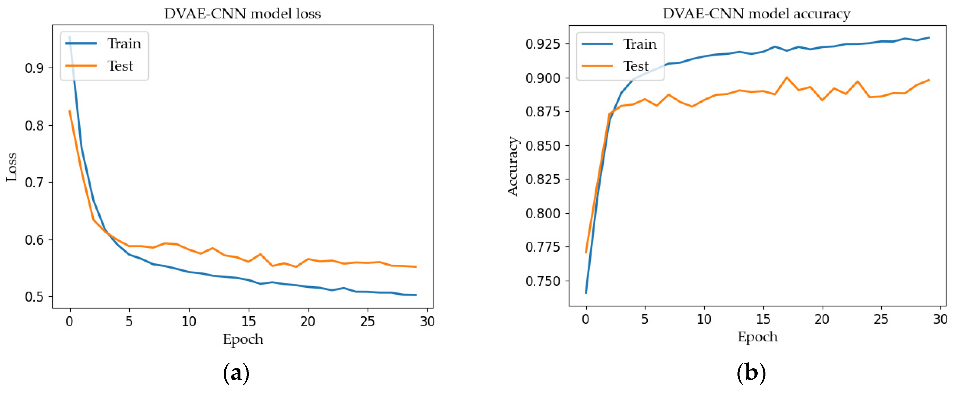
4.1.2. Model Training and Performance Comparison

The purpose of training the localization model is to obtain a set of parameters so that the classification accuracy of the model meets our localization requirements. Several architectures with a different number of layers are compared in order to make the proposed model as lightweight as possible. To make it more effective in real-time applications in terms of speed and accuracy, the hyperparameter settings for the final model structure are shown in the

Table 1. Hyperparameters of the DVAE-CNN model.

Model	Hyperparameters	Values of Parameters
DVAE-CNN	Input Size	25 × 25 (according to map)
	Convolutional layer	3 × 3 filter size, stride = 2
	Latent_dim	20
	Activation Function	ReLU (rectified liner unit)
	Number of Convolutional Layers	2
	Pooling Size	2
	Dropout	0.5
	Number of FC Layers	2
	Optimizer	Adam
	Learning Rate	0.0001
	Batch Size	32
	Epochs	500 (EarlyStopping, patience = 10, verbose = 1)
Classification Layer	Input Size	Latent_dim (20,1)
	Convolutional layer	Filter size = 32, kernel size = 5
	Max pooling1D	Pool size = 5
	Dropout	0.03
	Number of FC Layers	7
	Loss	Mean_squared_error
	Optimizer	Adam (7 × 10−4)
	Activation Function	ReLU (Rectified Liner Unit)

.

The deep learning library Kreas is used as a tool for building network models. In the construction of a DVAE-CNN network, the input layer, encoding and decoding layers composed of convolutional networks are designed. Among them, feature extraction is realized by multi-layer convolution operation, which converts the data into input images in 25 × 25 format and adds Gaussian noise. When building the encoder, in the first convolutional layer, the image is first convolved with 2 3 × 3 convolution kernels and 2 × 2 max pooling (strides = 2). The part that is not enough of a convolution kernel size is discarded, and then the second layer repeats the operation. Among them, the decoder is then constructed, which takes the result of the encoder as the input and outputs the data without added noise. The ReLU activation function is also used, which makes neurons have a sparse activation. Moreover, in order to prevent over fitting, complex model structures are not used. In addition, the dropout value of 0.5 after the full connection layer, the learning rate is 0.0001, and the loss function is the sum of the reconstruction loss and KL loss. The training model uses the backpropagation algorithm to train the entire network, and the training model is able to find the non-linear mapping relationship between the class and location information representing the reference. That is, when the change in loss function between two adjacent calculations is less than the set threshold or reaches a certain number of iterations, the network is stable, and the network parameters are saved. In order to save time and resources, the method of stopping training in advance is adopted, and the method of cross-validation is used to train repeatedly until the model converges.

When training the locator, the output of the encoder, that is, the latent feature constructed by the mean and variance in the latent space, is used as the input of the 1D convolutional network, and the output is the 2D coordinates of the positioning result. The dimension of the latent spatial feature is set to 20 in this paper. The ReLU activation function is used as the activation function, and 32 5 × 5 convolution kernels are connected to 7 fully connected layers after the convolution operation to extract the non-linear features. Finally, after configuring the loss and optimizer, the training starts. When the model converges, the sampling is stopped in advance. The 10-foldCV is determined by Stratified k-fold cross validation scores, i.e., 90% of the data are used for training and 10% for testing at each iteration. Finally, the trained model is encapsulated into an executable file for the real-time location. The training process of the model is shown in Figure 16.

As can be seen from Figure 16, the initial loss is reduced from 0.98 to 0.51, and the accuracy finally reaches 92.58%, which verifies that the model has a high classification accuracy for non-linear and non-stationary multi-dimensional atlas signals. To compare the performance advantages of the proposed model, the proposed DVAE-CNN and multiple representative models, including AE (autoencoder), VAE (variational autoencoder), AE-CNN (CNN-assisted autoencoder) and VAE-CNN (CNN-assisted variational autoencoder) are compared based on the electromagnetic atlas dataset constructed in the previous section. Due to the randomness of the sample selection, each algorithm is executed 10 times and its identification results are observed. According to previous research, the AE network structure is set as: 256-2048-200-100-80-2, including 1 input layer, 4 hidden layers and 1 output layer, the activation function is RELU, batch_size = 32, epoch = 500. The VAE network structure is set as: 256-1024-200-100-80-2, including 1 input layer, 4 hidden layers and 1 output layer. In the AE-CNN, the encoder network structure is set to: 256-1024-200-100-80-20, including 1 input layer, 3 hidden layers and 1 output layer. The 1DCNN structure is consistent with the classification CNN structure, and the output dimension is 2. The VAE-CNN model structure is consistent with the DVAE-CNN, only the part that increases the noise is removed. For each model, the positioning accuracy on the validation set will be recorded, and the standard for evaluating the positioning accuracy of the model is shown in Equation (14), and the final test result is shown in Figure 17.

$$Accuracy=\sqrt{{\left(x-x_0\right)}^2+{\left(y-y_0\right)}^2}$$

(14)

Among them, $\left(x,y\right)$ is the abscissa and ordinate of the model prediction, and $\left(x_0,y_0\right)$ is the abscissa and ordinate of the actual value.

Figure 17. Comparison of positioning accuracy of different models.

Figure 17. Comparison of positioning accuracy of different models.

As can be seen from Figure 17, the AE model has no regularization of the latent variables in the latent space, so that the latent space features of the different positions may not correspond to the positions, so the existence of fuzzy positions leads to large classification errors. The latent spatial features of the VAE are forced to be regularized by the relevant parameter settings. By optimizing the reconstruction loss and the KL loss, there is no gap between the distributions of the latent space features, and similar data will be superimposed in the same area, and the accuracy is relatively high. After combining with the CNN, the overall positioning accuracy has been significantly improved, and the average positioning accuracy has reached 1.29 m and 1.18 m, respectively, which verifies that the CNN plays a key role in the identification of the structured features of the electromagnetic atlas. After adding the denoising ability of the model to the data containing noise, the average positioning performance is further improved by 7.8%, and the dispersion of the positioning error is lower, which verifies the effectiveness of the model. In the case of a complete multi-dimensional signal reception and small environmental interference, the positioning result can achieve accurate matching with the reference position, and the positioning accuracy can achieve centimeter level. The specific comparison is shown in

Table 2. Comparison and analysis of positioning performance of various models.

Different Methods	Positioning Accuracy Using Different Methods (m)
	Maximum	Minimum	Mean
AE + Classifier	6.00	0.03	2.35
VAE + Classifier	5.12	0.04	2.28
AE-CNN	3.62	0.05	1.29
VAE-CNN	2.71	0.03	1.18
Our method	2.70	0.03	1.07

.

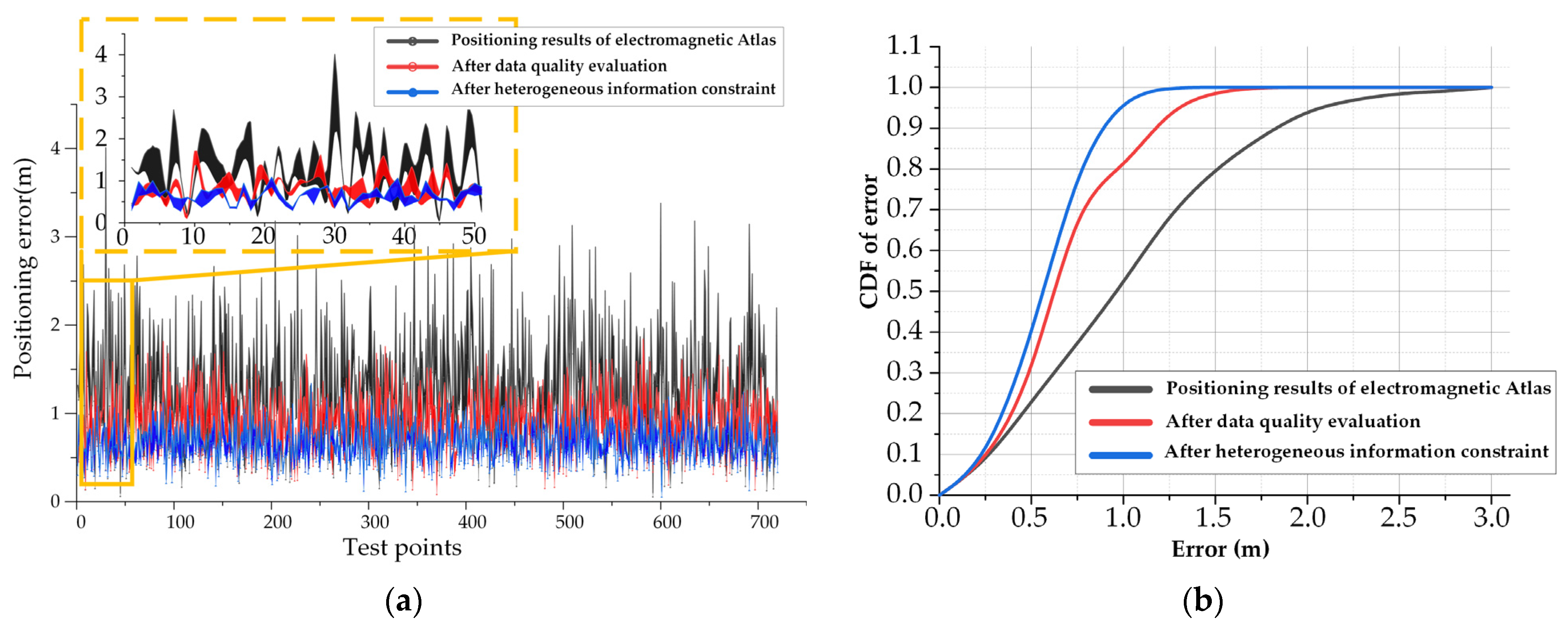
4.1.3. Analysis on the Effectiveness of Credible Evaluation Methods

In order to compare the effective constraints of the credible evaluation method on the positioning results, relevant experiments were carried out in the test field environment. After introducing the multi-dimensional graph evaluation model and the assistance of heterogeneous information, the positioning results of the set test trajectory are constrained. In order to further verify the effectiveness of the credible evaluation method in the real environment, this paper conducts a comparative test in the experimental environment, and the test results are shown in Figure 18.

As can be seen from Figure 18, the orange line is the reference track, and the positioning coordinate system is the Gaussian plane rectangular coordinate system. The black track is the positioning track of the multi-dimensional atlas, the position deviation is large and there are results of passing through the wall; these results are considered unreliable. After adding the credible evaluation model, there is a red trajectory. Through the credible analysis and elimination of the multi-dimensional data, the data at the current moment are generated in combination with historical data to ensure the continuity of the positioning results. In order to further improve the reliability of the positioning results, heterogeneous information is introduced to constrain the positioning results. It can be seen that the positioning accuracy and reliability of the fusion system are significantly improved.

In order to analyze the effectiveness of the credible evaluation system more clearly, the error bands and error cumulative distribution functions of the three trajectories are drawn, as shown in Figure 19. The use of the error band instead of the error curve is to evaluate the positioning error more scientifically and objectively through the confidence interval. The blue trajectory is the result after being constrained by the credible evaluation method. The average positioning error is 0.56 m, the maximum positioning error is 1.25 m and 95.2% of the errors are less than 1 m. Compared with the positioning results without additional evaluation, the average positioning accuracy is improved by 74.6%.

In addition, in terms of the reliability evaluation of the positioning system, it is defined as the percentage of the time when the system positioning error is less than the reliability threshold to the total observation time within a certain period of time in the specified area. When the reliability threshold is set to 1 m, the positioning reliability is improved by 88.2% after the credible evaluation is added, which verifies the effectiveness of the evaluation system.

4.1.4. Fusion Positioning Performance Evaluation

In order to verify the effectiveness of the multi-dimensional data fusion and the localization performance comparison with relatively advanced algorithms, a comparative experiment is carried out on the individual pseudolite carrier difference fingerprints [27], carrier phase difference search [28] and positioning method of fixed z-axis with known initial point [29]. Among them, a CVAE-based fingerprint positioning method is proposed in [27], which realizes the positioning by performing feature matching on multiple sets of carrier differences. In [28], an iterative search method based on the carrier difference between epochs is proposed to realize the continuous positioning. The literature [29] proposed a Doppler velocity measurement positioning method, which realizes the position prediction by measuring the target velocity and initial position.

In order to ensure the rationality of the experiment, this paper reproduces the relevant algorithms according to the parameter settings in the various literatures in the same experimental environment, and the experimental results are shown in Figure 20.

As can be seen from Figure 20, the Epoch-CPDS and Z-KPI algorithms proposed in [28,29] did not consider the localization problem in non-LOS environments. Therefore, in the test environment of this paper, the errors of these two algorithms are relatively large, and the average errors are 3.41 m and 3.38 m, respectively. The Inter-satellite CPDM algorithm proposed in document [27], since abnormal situations such as a signal loss of lock and environmental interference are not considered, the average positioning accuracy is 1.29 m, and the maximum error is 3.32 m. Compared with other methods, the method in this paper not only improves the coverage of high-precision positioning, but also improves the reliability of the positioning system. Compared with the three methods [27,28,29], the average positioning accuracy is improved by about 56%, 83.5% and 82.9%, respectively. The specific analysis is shown in the

Table 3. Comparison and analysis of positioning accuracy of various methods.

Algorithm	Mean Error (m)	90% Error (m)	Maximum Error (m)
Inter-satellite CPDM [27]	1.29	2.25	3.69
Epoch-CPDS [28]	3.42	5.00	7.82
Z-KPI [29]	3.38	5.26	7.21
Our Method	0.56	1.02	1.23

.

4.2. Positioning Performance Analysis in Real Application Scenarios

In order to verify the effect of the positioning system designed in this paper in practical applications, an application demonstration was carried out with the help of the indoor area of the venue of the Beijing 2022 Winter Olympics. Based on this positioning system, it can provide location services such as emergency command and dispatch, epidemic prevention and control, unmanned distribution and security control during the event. The venue environment is shown in Figure 21. The indoor area is about 10,000 square meters, with a total of about 16 floors. The electromagnetic environment in the venue meets the requirements of the National Radio Regulatory Commission. Based on the pseudolites, Wi-Fi and geomagnetic information in the site, a multi-dimensional electromagnetic field atlas was constructed to provide data support for high-precision positioning.

In the early deployment stage of this positioning system, the positioning capabilities of a variety of typical areas, such as indoor open areas, indoor long and narrow areas and indoor and outdoor transition areas, were tested, as shown in Figure 22.

5. Conclusions

Aiming at the problem of the low robustness of single signal source positioning performance in indoor/underground GNSS navigation signal rejection environments, a multi-level fusion positioning method based on a multi-dimensional electromagnetic atlas is proposed. A method for the dynamic acquisition and construction of a multi-dimensional electromagnetic atlas is designed. The DVAE-CNN model is used for deep feature recognition and fusion, and the mapping relationship between the spatial position and hidden features is constructed, thereby reducing the influence of environmental factors on the original observation information and improving the accuracy of the positioning system. Finally, about 90% of the positioning errors in various typical indoor environments are better than 1 m, and the average positioning error in the environment including non-LOS is 0.56 m. Compared with the current, more advanced positioning methods, the average positioning accuracy is improved by about 56%, 83.5% and 82.9%, respectively, which verifies the effectiveness of the algorithm. At the same time, the system was successfully applied to the venues of the 2022 Beijing Winter Olympics, providing high-precision location services for indoor and outdoor areas. It has to be said that the current positioning system still faces some challenges in practical use. For example, during the positioning process, the terminal antenna must not be blocked. When the terminal is placed in the user’s pocket or bag, the real-time positioning data will not be enough to ensure the positioning accuracy. These problems are also the difficulties faced by the current navigation and positioning.

References

1. Huang, L.; Li, H.; Yu, B.; Gan, X.; Wang, B.; Li, Y.; Zhu, R. Combination of smartphone MEMS sensors and environmental prior information for pedestrian indoor positioning. Sensors 2020, 20, 2263. [Google Scholar] [CrossRef] [Green Version]
2. Alarifi, A.; Al-Salman, A.; Alsaleh, M.; Alnafessah, A.; Al-Hadhrami, S.; Al-Ammar, M.A.; Al-Khalifa, H.S. Ultra wideband indoor positioning technologies: Analysis and recent advances. Sensors 2016, 16, 707. [Google Scholar] [CrossRef] [Green Version]
3. Ijaz, F.; Yang, H.K.; Ahmad, A.W.; Lee, C. Indoor positioning: A review of indoor ultrasonic positioning systems. In Proceedings of the 2013 15th International Conference on Advanced Communications Technology (ICACT), PyeongChang, Korea, 27–30 January 2013; pp. 1146–1150. [Google Scholar]
4. Basiri, A.; Lohan, E.S.; Moore, T.; Winstanley, A.; Peltola, P.; Hill, C.; e Silva, P.F. Indoor location based services challenges, requirements and usability of current solutions. Comput. Sci. Rev. 2017, 24, 1–12. [Google Scholar] [CrossRef] [Green Version]
5. Billa, A.; Shayea, I.; Alhammadi, A.; Abdullah, Q.; Roslee, M. An overview of indoor localization technologies: Toward IoT navigation services. In Proceedings of the 2020 IEEE 5th International Symposium on Telecommunication Technologies (ISTT), Shah Alam, Malaysia, 9–11 November 2020; pp. 76–81. [Google Scholar]
6. Shang, S.; Wang, L. Overview of WiFi fingerprinting-based indoor positioning. IET Commun. 2022, 16, 725–733. [Google Scholar] [CrossRef]
7. Ren, Y.; Salim, F.D.; Tomko, M.; Bai, Y.B.; Chan, J.; Qin, K.K.; Sanderson, M. D-Log: A WiFi Log-based differential scheme for enhanced indoor localization with single RSSI source and infrequent sampling rate. Pervasive Mob. Comput. 2017, 37, 94–114. [Google Scholar] [CrossRef]
8. Yang, T.; Cabani, A.; Chafouk, H. A Survey of Recent Indoor Localization Scenarios and Methodologies. Sensors 2021, 21, 8086. [Google Scholar] [CrossRef] [PubMed]
9. Witrisal, K.; Hinteregger, S.; Kulmer, J.; Leitinger, E.; Meissner, P. High-accuracy positioning for indoor applications: RFID, UWB, 5G, and beyond. In Proceedings of the 2016 IEEE International Conference on RFID (RFID), Orlando, FL, USA, 3–5 May 2016; pp. 1–7. [Google Scholar]
10. Pascacio, P.; Casteleyn, S.; Torres-Sospedra, J.; Lohan, E.S.; Nurmi, J. Collaborative indoor positioning systems: A systematic review. Sensors 2021, 21, 1002. [Google Scholar] [CrossRef]
11. Mandal, A.; Lopes, C.V.; Givargis, T.; Haghighat, A.; Jurdak, R.; Baldi, P. Beep: 3D indoor positioning using audible sound. In Proceedings of the Second IEEE Consumer Communications and Networking Conference, CCNC, Las Vegas, NV, USA, 6 January 2005; pp. 348–353. [Google Scholar]
12. Rossi, M.; Seiter, J.; Amft, O.; Buchmeier, S.; Tröster, G. RoomSense: An indoor positioning system for smartphones using active sound probing. In Proceedings of the 4th Augmented Human International Conference, New York, NY, USA, 7–8 March 2013; pp. 89–95. [Google Scholar]
13. Kim, H.G.; Kim, G.Y. Deep neural network-based indoor emergency awareness using contextual information from sound, human activity, and indoor position on mobile device. IEEE Trans. Consum. Electron. 2020, 66, 271–278. [Google Scholar] [CrossRef]
14. Faragher, R.; Harle, R. An analysis of the accuracy of bluetooth low energy for indoor positioning applications. In Proceedings of the 27th International Technical Meeting of The Satellite Division of the Institute of Navigation (ION GNSS+ 2014), Tampa, FL, USA, 8–12 September 2014; pp. 201–210. [Google Scholar]
15. Subhan, F.; Hasbullah, H.; Rozyyev, A.; Bakhsh, S.T. Indoor positioning in bluetooth networks using fingerprinting and lateration approach. In Proceedings of the 2011 International Conference on Information Science and Applications, Jeju, Korea, 26–29 April 2011; pp. 1–9. [Google Scholar]
16. Puckdeevongs, A.; Tripathi, N.K.; Witayangkurn, A.; Saengudomlert, P. Classroom attendance systems based on Bluetooth Low Energy Indoor Positioning Technology for smart campus. Information 2020, 11, 329. [Google Scholar] [CrossRef]
17. Bocquet, M.; Loyez, C.; Benlarbi-Delai, A. Using enhanced-TDOA measurement for indoor positioning. IEEE Microw. Wirel. Compon. Lett. 2005, 15, 612–614. [Google Scholar] [CrossRef]
18. Zhou, Z. An Overview of Ultra-Wideband Positioning Technology and Its Applications. In SHS Web of Conferences; EDP Sciences: Paris, France, 2022; Volume 144, p. 02001. [Google Scholar]
19. Alamu, O.; Iyaomolere, B.; Abdulrahman, A. An overview of massive MIMO localization techniques in wireless cellular networks: Recent advances and outlook. Ad Hoc Netw. 2021, 111, 102353. [Google Scholar] [CrossRef]
20. Huang, L.; Yu, B.; Li, H.; Zhang, H.; Li, S.; Zhu, R.; Li, Y. HPIPS: A high-precision indoor pedestrian positioning system fusing WiFi-RTT, MEMS, and map information. Sensors 2020, 20, 6795. [Google Scholar] [CrossRef] [PubMed]
21. Li, C.T.; Cheng, C.P.; Chen, K. Top 10 technologies for indoor positioning on construction sites. Autom. Constr. 2020, 118, 103309. [Google Scholar] [CrossRef]
22. Farid, Z.; Nordin, R.; Ismail, M. Recent advances in wireless indoor localization techniques and system. J. Comput. Netw. Commun. 2013, 2013, 185138. [Google Scholar] [CrossRef]
23. Poulose, A.; Eyobu, S.; Han, D.S. A combined PDR and Wi-Fi trilateration algorithm for indoor localization. In Proceedings of the 2019 International Conference on Artificial Intelligence in Information and Communication (ICAIIC), Okinawa, Japan, 11–13 February 2019; pp. 72–77. [Google Scholar]
24. Diaz, E.M.; Ahmed, D.B.; Kaiser, S. A review of indoor localization methods based on inertial sensors. Geogr. Fingerpr. Data Creat. Syst. Indoor Position Indoor/Outdoor Navig. 2019, 2019, 311–333. [Google Scholar]
25. Ouyang, G.; Abed-Meraim, K. A Survey of Magnetic-Field-Based Indoor Localization. Electronics 2022, 11, 864. [Google Scholar] [CrossRef]
26. Luo, R.C.; Hsu, W.L. Robust Indoor Localization Using Histogram of Oriented Depth Model Feature Map for Intelligent Service Robotics. IEEE/ASME Trans. Mechatron. 2022, 27, 4033–4044. [Google Scholar] [CrossRef]
27. Huang, L.; Gan, X.; Yu, B.; Zhang, H.; Li, S.; Cheng, J.; Wang, B. An innovative fingerprint location algorithm for indoor positioning based on array pseudolite. Sensors 2019, 19, 4420. [Google Scholar] [CrossRef] [Green Version]
28. Yu, X.; Feng, X.; Deng, Z. Research on Indoor Positioning Algorithm Based on Pseudolites. Radio Eng. 2020, 50, 85–89. [Google Scholar]
29. Gan, X.; Yu, B.; Wang, X.; Yang, Y.; Jia, R.; Zhang, H.; Wang, B. A new array pseudolites technology for high precision indoor positioning. IEEE Access 2019, 7, 153269–153277. [Google Scholar] [CrossRef]
30. Shum, L.C.; Faieghi, R.; Borsook, T.; Faruk, T.; Kassam, S.; Nabavi, H.; Iaboni, A. Indoor Location Data for Tracking Human Behaviours: A Scoping Review. Sensors 2022, 22, 1220. [Google Scholar] [CrossRef] [PubMed]
31. Alhammadi, A.; Hashim, F.; Rasid, A.M.F.; Alraih, S. A three-dimensional pattern recognition localization system based on a Bayesian graphical model. Int. Ournal Distrib. Sens. Netw. 2020, 16, 1550147719884893. [Google Scholar] [CrossRef]
32. Arigye, W.; Pu, Q.; Zhou, M.; Khalid, W.; Tahir, M.J. RSSI Fingerprint Height Based Empirical Model Prediction for Smart Indoor Localization. Sensors 2022, 22, 9054. [Google Scholar] [CrossRef] [PubMed]
33. Kuang, J.; Niu, X.; Zhang, P.; Chen, X. Indoor positioning based on pedestrian dead reckoning and magnetic field matching for smartphones. Sensors 2018, 18, 4142. [Google Scholar] [CrossRef] [PubMed] [Green Version]
34. Birkel, U.; Weber, M. Indoor localization with UMTS compared to WLAN. In Proceedings of the 2012 International Conference on Indoor Positioning and Indoor Navigation (IPIN), Sydney, NSW, Australia, 13–15 November 2012; pp. 1–6. [Google Scholar]
35. Song, W.; Lee, H.; Lee, S.H.; Choi, M.H.; Hong, M. Implementation of android application for indoor positioning system with estimote BLE beacons. J. Internet Technol. 2018, 19, 871–878. [Google Scholar]
36. Xia, H.; Zuo, J.; Liu, S.; Qiao, Y. Indoor localization on smartphones using built-in sensors and map constraints. IEEE Trans. Instrum. Meas. 2018, 68, 1189–1198. [Google Scholar] [CrossRef]
37. Gusenbauer, D.; Isert, C.; Krösche, J. Self-contained indoor positioning on off-the-shelf mobile devices. In Proceedings of the 2010 International Conference on Indoor Positioning and Indoor Navigation, Zurich, Switzerland, 15–17 September 2010; pp. 1–9. [Google Scholar]
Figure 1. Spatial distribution of PL carrier phase data.
Remotesensing 15 00353 g001
Figure 2. Spatial distribution of Wi-Fi signal strength.
Remotesensing 15 00353 g002
Figure 3. Spatial distribution of geomagnetic data.
Remotesensing 15 00353 g003
Figure 4. Structure of indoor positioning system considering credible evaluation.
Remotesensing 15 00353 g004
Figure 5. Schematic diagram of multi-dimensional electromagnetic atlas positioning.
Remotesensing 15 00353 g005
Figure 6. Schematic diagram of multi-dimensional data collection.
Remotesensing 15 00353 g006
Figure 7. Construction method of multi-dimensional electromagnetic atlas.
Remotesensing 15 00353 g007
Figure 8. DVAE-CNN model construction and pre-training process.
Remotesensing 15 00353 g008
Figure 9. Locator model training process.
Remotesensing 15 00353 g009
Figure 10. Flowchart of mobile application of positioning model.
Remotesensing 15 00353 g010
Figure 11. Multi-dimensional atlas credible assessment model.
Remotesensing 15 00353 g011
Figure 12. Schematic of PDR.
Remotesensing 15 00353 g012
Figure 13. Trusted evaluation mechanism based on heterogeneous information.
Remotesensing 15 00353 g013
Figure 14. Test environment: (a) 1st floor of test field; (b) 2nd floor of test field.
Remotesensing 15 00353 g014
Figure 15. Construction of multi-dimensional atlas dataset.
Remotesensing 15 00353 g015
Figure 16. DVAE-CNN model: (a) loss curves; (b) accuracy curves.
Remotesensing 15 00353 g016
Figure 18. Positioning trajectory considering the credible evaluation mechanism.
Remotesensing 15 00353 g018
Figure 19. Error Analysis: (a) Error band; (b) Error cumulative distribution function.
Remotesensing 15 00353 g019
Figure 20. Effectiveness test of multi-dimensional information fusion data [27,28,29].
Remotesensing 15 00353 g020
Figure 21. Application of indoor positioning system for 2022 Winter Olympics.
Remotesensing 15 00353 g021
Figure 22. Localization results of multiple typical indoor and outdoor scenes.
Remotesensing 15 00353 g022