First-Break Picking of Large-Offset Seismic Data Based on CNNs with Weighted Data

Abstract

Deep reflection seismic data are usually accompanied by large-offset data, and the accurate and rapid identification of the first arrivals of seismic records plays an important role in eliminating the effects of topography and other factors that increase with the increasing offsets. In this paper, we propose a method based on convolutional neural networks (CNNs) that can accurately identify the first arrivals of large-offset seismic data. A time window for linear dynamic correction was established to convert the raw seismic data into rectangular images so as to reduce the amount of invalid sample data and improve the training efficiency. In order to enhance the prediction effect of the far-offset first arrivals, we propose the strategy of adjusting the weight of the far-offset data to increase the weight of the far-offset data in the training dataset and, thus, to improve the first arrival accuracy. The manually picked first arrivals are used as labels and the input to the CNNs for training, and the full-offset first arrivals are the output. The travel time tomography velocity is modeled and compared based on the first arrivals obtained through manual picking, industrial software automatic picking, and CNN prediction. The results show that the application of CNNs to large-offset seismic datasets can help researchers to obtain the first arrivals at different offsets, while the inclusion of far-offset weights can effectively improve the modeling depth of the tomography inversion, and the accuracy of the results is high.

1. Introduction

Since the 1970s, many countries have successively carried out continental crustal exploration programs using deep seismic reflection technology. Deep reflection seismic exploration is a kind of seismic exploration technology that uses a large amount of a given explosive source to excite high-energy seismic waves so that they can propagate within the interior of the earth over a long distance. Its detection depth can reach close to the Moho surface, and it is a kind of seismic exploration technology used to explore the deep earth tectonic structure and continental plate undulation [1,2,3,4,5,6,7,8,9]. However, due to the long range of the line placements in deep reflection exploration and the complex structure of elevation differences, and decreasing velocity zones within the work area, the signal-to-noise ratio of long-offset data is often very low, and it is usually necessary to build a tomographic model in order to solve the static correction problem and improve the deep imaging effect. This requires the accurate identification of the first arrivals of the seismic data.

Seismic first arrivals are the direct or refracted signals that arrive first among all the signals received by the detector. Accurate first-break picking is an important process in the pre-processing stage of seismic exploration, and the results can be applied to problems such as static correction, tomographic imaging, and hypocentral location analysis. In the early exploration work, first-break picking was usually performed by experienced professionals who manually judged the type of seismic waves and, thus, picked up the first arrivals through numerous years of work. However, this method undoubtedly consumes a great deal of manpower and time. At present, as the scale of seismic exploration continues to expand and exploration technology continues to improve, the dimensionality and magnitude of seismic exploration data have increased dramatically, and the manual first-break picking method can no longer meet the needs of production in a timely manner. Therefore, the study of automatic picking methods that can accurately identify the first arrivals of seismic waves is an issue of great interest.

Over the past few decades, researchers have developed many semi-automatic and automatic algorithms for identifying first arrivals by analyzing the physical characteristics of seismic traces. A classical algorithm is the short-time and long-time average ratio (STA/LTA), which has been tested and proven to be effective [10,11,12]. In addition, there are some first-break picking algorithms, such as statistical detection [13], the K-mean eigenfunctions [14], before-and-after waveform energy ratio method [15,16], autoregressive techniques, and domain value conversion techniques, etc. All these methods have achieved certain application results in production, but they all have their own limitations. The main limitation is that most methods analyze a single seismic trace, ignoring the important property of spatial correlation between neighboring trace sets, resulting in some pickups that do not equate to the true or empirically determined first-break points. In other cases, they are limited by the data quality and cannot be used to obtain good results under low-signal-to-noise-ratio conditions. In addition, with the increase in the complexity of the work area, the workload of first-break picking is increasing, and the current algorithms, although they can adapt to the low-signal-to-noise-ratio conditions, are still computationally inefficient and even more unsuitable for the current technology, which is the most important problem faced by researchers using the traditional first-break automatic picking methods.

Since Hinton formally introduced the concept of deep learning in 2006, various geophysical processing techniques based on deep learning have been proposed [17]. The use of neural networks for first-break picking was studied early on (Michael et al., 1993). The use of artificial neural networks (ANNs) for first-break picking was studied even earlier, and this technology has been applied to controlled seismic sources, as well as microseismic data [18]. This type of method analyzes the skeleton characteristics of seismic traces, such as the STA/LTA ratio, statistical parameters, skewness, and attributes such as the amplitude and frequency of the signal, as inputs to the ANNs and classifies the first arrivals based on this information. Although such methods can adaptively classify different types of first arrivals, they are similar in concept to the traditional methods of judging the physical information of single seismic traces and still do not take advantage of the spatial correlation between seismic waveforms [19,20,21]. Convolutional neural networks (CNNs) are effective om extracting a certain range of data features for the purpose of recognition, and CNN trainers based on machine learning and deep learning have been studied for waveform classification, multichannel recognition, error repair, and microseismic recognition [22,23,24]. In addition, there are studies on automatic first-break picking based on methods such as support vector machines, convolutional image segmentation, and U-Net networks [25,26]. However, in the existing studies, only the near-offset data with good signal-to-noise ratios were tested. In the case of large-offset data, the far offsets are usually accompanied by very strong background noise, which is not applicable to the traditional first arrival methods, and the question of whether the deep learning methods can be applied to the recognition of the first arrivals of such complex seismic data needs to be tested.

In this study, we constructed a deep CNN and applied it to a two-dimensional seismic dataset with large offsets, highly developed background noise, and complex data features. Firstly, we pre-processed the seismic data and used the linear time window correction method to linearly correct the seismic data before picking up the first arrivals, smoothing out the first arrival time of the overall gun set, thus benefiting from the application of automatic picking and manual discriminatory modification correction. Secondly, we constructed a weight matrix to increase the weight of the far-offset data among the training data, providing the network with sufficient far-offset information for first-break pick up learning. Then, we built the network architecture of the CNN and set the relevant hyperparameters. After that, we conducted the first-break picking test of the large-offset seismic data based on the trained CNN and assessed the results obtained from the tomography images, which we compared with the picking results obtained by other methods. Finally, here, we summarize the conclusions obtained from the experiments.

2. Theory and Methods

2.1. Basic Principles of CNNs

Convolutional neural networks (CNNs) have representational learning capabilities and can perform the translation-invariant classification of input data according to their hierarchical structure, as well as supervised and unsupervised learning. The shared parameters of convolutional kernels and the sparsity of inter-layer connections within their hidden layers allow CNNs to learn features with a small number of calculations, such as the pixels and audio. They produce stable results without additional feature engineering requirements in regard to the data and are used in a large number of applications in computer vision, natural language processing, and other fields. Compared with other networks, the greatest advantage of CNNs is that they require fewer training parameters with a high efficiency. Thus, CNNs are still very popular deep learning models. A CNN model mainly includes a convolutional layer, a pooling layer, and a fully connected layer.

2.1.1. Convolutional Layer

The convolutional layer is the most important layer in the whole neural network, and the core part of this layer is the filter, or the so-called the convolutional kernel. The convolutional kernel has two properties, namely the size and depth, which are specified manually, while the weight parameters are randomly generated by the program during initialization, and these weights are continuously optimized in the later stage of the training process to achieve the best classification results. After the convolution calculation is completed, a function used to correct the linear unit is often added to non-linearize the data. The corresponding formula for the convolution layer is:

$${\mathrm{x}}_{\mathrm{j}}^{\mathrm{l}}=\mathrm{g}\left({\mathrm{x}}_{\mathrm{i}}^{\mathrm{l}-1}{\ast \mathrm{W}}_{\mathrm{ij}}^{\mathrm{l}}+{\mathrm{b}}_{\mathrm{j}}^{\mathrm{l}}\right)$$

(1)

where ${\mathrm{x}}_{\mathrm{i}}^{\mathrm{l}-1}$ is the output of the i-th neuron in layer $\mathrm{l}-1$, ${\mathrm{x}}_{\mathrm{j}}^{\mathrm{l}}$ is the output of the $\mathrm{j}$-th neuron in layer$\mathrm{l}$ after the convolutional operation, ${\mathrm{W}}_{\mathrm{ij}}^{\mathrm{l}}$ is the convolutional kernel, ${\mathrm{b}}_{\mathrm{j}}^{\mathrm{l}}$ is the bias, $\ast$ is the convolutional operation, and $\mathrm{g}$ is the activation function. The commonly used activations are the tanh function, sigmoid function, relu function, etc. Among these, the formula of the tanh activation function is defined as:

$$\mathrm{g}\left(\mathrm{x}\right)=\frac{{\mathrm{e}}^{\mathrm{x}}-{\mathrm{e}}^{-\mathrm{x}}}{{\mathrm{e}}^{\mathrm{x}}+{\mathrm{e}}^{-\mathrm{x}}}$$

(2)

Compared with the other two activation functions, the output interval of the tanh function is in the rage of (−1, 1), having a 0 mean, which allows it to completely outperform the sigmoid function in the hidden layers of the neural network, matching the seismic data characteristics.

In the case of convolutional layers, the feature graph of the network usually becomes deeper, allowing for deeper analysis of the input data and adequate feature extraction. The initial values of the weights and biases in the convolutional kernel are set during training, and the weights and biases in the convolutional kernel are continuously adjusted during training to achieve the best performance of the network.

2.1.2. Pooling Layer

In order to effectively reduce the network volume and the computation and improve the computation efficiency, CNNs set the pooling operation after the convolution layer. Common pooling operations include average pooling and maximum pooling, with average pooling being the average of the local features and maximum pooling being the maximum of the local features. The parameters of the pooling layer are not involved in the update iteration. Instead, this stage involves only an operation rule, which can reduce the training parameters and complexity of the network and, to some extent, improve the generalization ability of the model.

2.1.3. Fully Connected Layer

The fully connected layer is responsible for rearranging the extracted features and performing the classification, regression, or mapping of the network. After the convolution and pooling operations, the feature graph is tiled as a one-dimensional vector as the input to the fully connected layer, where each neuron is fully connected to all the neurons in the next layer. According to the task requirements, the appropriate number of fully connected layers and output layer neuron nodes are set to complete the corresponding classification or regression task, which is calculated as follows:

$${\mathrm{x}}_{\mathrm{j}}^{\mathrm{l}}=\mathrm{f}\left({\mathrm{W}}_{\mathrm{ij}}^{\mathrm{l}}{\mathrm{x}}_{\mathrm{i}}^{\mathrm{l}-1}+{\mathrm{b}}_{\mathrm{j}}^{\mathrm{i}}\right)$$

(3)

where ${\mathrm{x}}_{\mathrm{j}}^{\mathrm{l}-1}$ is the output of the $\mathrm{i}$-th neuron in layer$\mathrm{l}-1$,${ \mathrm{x}}_{\mathrm{j}}^{\mathrm{l}}$ is the output of the$\mathrm{j}$-th neuron in layer$\mathrm{l}$ after a fully connected layer, ${\mathrm{W}}_{\mathrm{ij}}^{\mathrm{l}}$ is the weight matrix, ${\mathrm{b}}_{\mathrm{j}}^{\mathrm{l}}$ is the bias, and$\mathrm{f}$ is the activation function.

To avoid overfitting, the fully connected layer is usually subjected to a random deactivation technique (dropout). Dropout is a regularization technique that reduces the complexity of the model by setting the size of the dropout value so that some nodes in the network do not participate in the training process of the CNN.

2.2. Processing Flow

2.2.1. Sample Set Production

The data used in this paper are 2D deep reflection seismic survey data, and the observation system is defined in the form of crooked lines. The length of the 2D survey line is approximately 100 km, and a total of 2921 detectors are deployed to receive the seismic data generated by 319 large explosive energy source excitations, with most of the track pitch being 50 m and the offsets of all the single-shot records being variable, in which the maximum offset can reach 40 km. Figure 1 shows the three single-shot records detected on the survey line. It can be seen that the signal-to-noise ratio is good in the case of the near offsets, and obvious background noise develops in the case of the far offsets, and it is difficult to identify the far-offset first arrivals because they are covered by noise. Overall, the signal-to-noise ratio of the data is poor, and the background noise, with surface wave interference, is highly developed. On the other hand, the data develop obvious multiple wave refraction signals, indicating the existence of high-speed regions in the subsurface. Additionally, the irregular shape of the first arrivals indicates the existence of surface fluctuation or the influence of strong downgradient zones. Thus, for this data set, we should focus on the long-wavelength static correction problems. Currently, the main methods used in industry to solve the long-wavelength static correction problem are first-break refractive wave static correction and first-break tomographic static corrections, both of which require accurate first arrivals to ensure that the correct field statics are obtained in order to observe the correct form of geological formations.

To address the above-mentioned issues, various pre-processing steps of this seismic data are required to facilitate the production of label graphs. The specific processes and methods are as follows:

(1)

Linear correction time window: When training the network, it is necessary to apply the seismic records and the corresponding first arrivals of the common shot point data to the trainer as inputs and labels, because the first arrivals only offer information such as direct waves and subsequently covered refraction waves, etc. If the full-time seismic data features are extracted for training, there will be a large amount of redundant information, and this will prolong the training time. Therefore, a linear correction time window was designed in this study to extract the seismic records close to the time of the first arrivals as the training input data. At the same time, the linear correction travel–time difference was determined according to the maximum left and right offset distances intercepted by the time window, the endpoint moments of the window function, and the difference in the seismic wave arrival time of the minimum offset so as to compress the seismic signals in the time field into a rectangular box, which can better utilize the spatial correlation of the first arrivals and reduce the input volume in order to improve the training efficiency. Figure 2 shows a comparison before and after the linear correction of the 130th and 190th shots. Although the time window does not flatten the intercepted first arrivals to a sufficient extent, it is very easy to handle, in the case of either single or multiple shots, by simply obtaining the first, last, and shot point first arrivals of each shot and then using these three values for the interception of the time window. In this paper, the time window is defined by time-shifting the timeline by $\tau /2$ in the upper and lower directions, respectively, and the mathematical expressions for the timeline and the linear correction time are calculated as:

$$\mathrm{W}\left(\mathrm{t}\right)=\{\begin{array}{c}{\mathrm{p}}_1{\mathrm{x}}_{\mathrm{i}}+{\mathrm{t}}_0 , {\mathrm{x}}_{\mathrm{i}}\le 0\\ {\mathrm{p}}_2{\mathrm{x}}_{\mathrm{i}}+{\mathrm{t}}_0 , { \mathrm{x}}_{\mathrm{i}}\ge 0\end{array}$$

(4)

$$\begin{gathered} {\mathrm{p}}_1=\left({\mathrm{t}}_{\mathrm{l}}-{\mathrm{t}}_0\right)/{\mathrm{x}}_{\mathrm{l}}, \\ {\mathrm{p}}_2=\left({\mathrm{t}}_0-{\mathrm{t}}_{\mathrm{r}}\right)/{\mathrm{x}}_{\mathrm{r}} \end{gathered}$$

(5)

$$\Delta \mathrm{t}=\{\begin{array}{c}\left(\tau ·{\mathrm{x}}_{\mathrm{i}}\right)/{\mathrm{x}}_{\mathrm{l}} , {\mathrm{x}}_{\mathrm{i}}\le 0\\ \left(\tau ·{\mathrm{x}}_{\mathrm{i}}\right)/{\mathrm{x}}_{\mathrm{r}} , {\mathrm{x}}_{\mathrm{i}}\ge 0\end{array}$$

(6)

where $W$ represents the time window function; $x$ represents the offset; $i$ is the trace index; $t_0$ represents the first arrivals at the minimum offset; $p_1$ and $p_2$ represent two different time line parameters; $x_l$ and $x_r$ represent the maximum left and right offsets of the time window intercept; $t_l$ and $t_r$ represent the first arrivals at the maximum offset; and $\Delta t$ is the degree of linear correction.

(2)

Increasing the weight of the far-offset data among the training data: Since seismic data have a good signal-to-noise ratio at the near offsets and a low signal-to-noise ratio at the far offsets, the effective signal is suppressed by noise, making it difficult to identify the first arrivals using traditional methods or industrial software. In order to improve the first-break picking accuracy of the network for the far offsets, in this paper, we propose a far-offset-data-weighting strategy, which sets all the single-shot records after the linear time window interception within 10 km of the shot location as the near-offset dataset and the rest as the far-offset dataset. In order to increase the weight of the far-offset data in the training dataset, the near-offset dataset of half of the single-shot records is randomly dropped from the training dataset, and the ratio of the near-offset dataset to the far-offset dataset is set as 1:2 to obtain the final training data. Weighting enables CNNs to learn more feature patterns of far offsets with a poor signal-to-noise ratio and the corresponding first arrivals, thus improving the prediction accuracy of the CNNs for far-offset first arrivals.

(3)

Seismic data trace editing: The detector is affected by environmental factors, the machine’s specific factors, and other factors during the work, and some invalid traces, bad traces, polarity reversal traces, etc., will appear in the data. In order to render the network unaffected by these traces, a certain number of invalid traces, abnormal data traces, polar traces, etc., are artificially added to the training data to improve the generalizability of the network.

(4)

Processing of the labels: In the process of generating labeled images, all the data points before the first arrivals are labeled as −1, and those after the first arrivals are labeled as 1. Figure 3 shows the results of the label data processing for the 190th shot. From the results, we can observe that the obtained labeled data appear to be white in the upper part and black in the lower part, and their size is consistent with the grayscale figure. The reason for this treatment is that [–1, 1] is consistent with the characteristics of seismic data, and this treatment is closer to a process of classifying the training data than that of directly outputting the first arrival time, which is more conducive to the extraction of first arrival features by the network model.

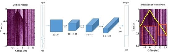
2.2.2. Network Construction

For the dataset established in this paper, we designed the convolutional neural network as a symmetric network with the same output data and data input size. In general, the hyperparameters of the convolutional neural network were variables determined based on experience and the effects of the test set. Different numbers of layers, learning rates, dropout deactivation rates, optimization methods, etc., can affect the final model results. In order to obtain the network structure with the best results, we conducted many tests using different hyperparameters. This paper only describes the effects of the different numbers of layers on the results, since using the most succinct convolutional neural network to achieve the study purpose is a popular method in research based on algorithms. The more layers there are, the higher the number of hidden layer nodes of the network and the stronger the learning ability of the network will be. However, at the same time, the network tends to fall to local minimums, and the learning speed can become very slow. We discuss two CNN network structures with different depths, named CNN-3 and CNN-4, respectively. Figure 4 shows the network models of CNN-3 and CNN-4, and their respective basic parameters are listed in

Table 1. CNN model parameters.

Layer Name	CNN-3	CNN-4
Input	[400 × 1 × 1] reshape Output: [20 × 20 × 1]
Conv1 + Pool1	[3 × 3, 32] max pool, stride 2 Output: [10 × 10 × 32]
Conv2 + Pool2	[3 × 3, 64] max pool, stride 2 Output: [5 × 5 × 64]
Conv3 + Pool3	[3 × 3, 128] max pool, stride 2 Output: [3 × 3 × 128]
Conv4 + Pool4	-	[3 × 3, 256] max pool, stride 2 Output: [2 × 2 × 256]
Ful1	[1024 × 1 × 1]
Ful2	[512 × 1 × 1]
Ful3	[480 × 1 × 1]
output	[400 × 1 × 1]

.

We trained these two networks separately, and their training samples and the other parameters involved in the training were exactly the same. In these networks, the activation functions are tanh functions, the loss functions are mean square difference functions, and the training algorithms are Adam optimization algorithms with a learning rate of 0.001. To prevent overfitting, the dropout strategy is used in the case of the fully connected layers, and the deactivation rate is set to 0.7. The loss values obtained after 200 iterations, respectively, are shown in Figure 5. It can be seen that CNN-3 has fewer layers, but it converges faster and more efficiently than CNN-4.

To provide a clearer picture of the effect of the pickup, the outputs of the network predictions are mapped according to the seismic records, and the results are shown in Figure 6. The left side of the figure shows the pickup prediction map for some of the traces based on the CNN-4 network, and the right side shows the results of the corresponding CNN-3. It can be seen that the pickup of CNN-4 is poor when there are strong noisy traces in the original seismic data, with obvious error fluctuations, while the results of CNN-3 are significantly better than those of CNN-4.

In order to represent the accuracy of the results more intuitively, the pickup correct rate metric was introduced in the experiments to evaluate the effectiveness of the models. The pickup correct rate is the ratio of the number of sample points where the error between the first-to-time point of the network prediction and the first-to-time point of the manual pickup is within two data points of the total number of pickup lanes. The correct pickup rate was calculated to be 92.8% for CNN-3 and 86.2% for CNN-4. In summary, the CNN-3 network model has a better pickup effect and higher pickup accuracy than CNN-4; thus, the CNN-3 network was finally selected in this paper.

3. Results

We applied the trained optimal network CNN-3 to the test set separated from the original shot sets. Among these, the test set has a total of 177 shots, and both the detector interval and the shot point interval are the same as those of the training set. The prediction results for the two single-shot records are shown in Figure 7. Among them, Figure 7a,e are the original records of two single shots; Figure 7b–d are the prediction results of the industrial software, unweighted CNN-3, and weighted CNN-3 based on Figure 7a; and Figure 7f–h are the prediction results of the industrial software, unweighted CNN-3, and weighted CNN-3 based on Figure 7e. The white, blue, and yellow circles represent the predictions provided by the industrial software, unweighted CNN-3, and weighted CNN-3, respectively, while the solid green line indicates the first arrivals carefully selected by manual picking from the direct and refracted waves of the seismic data. In the single figures, the small red boxes represent the zoomed-in position, and the large red boxes show the zoomed-in data. It can be seen that the industrial software performs poorly in the first-break picking of low-signal-to-noise-ratio, large-offset seismic data, while the prediction results provided by both the unweighted CNN-3 and the CNN-3 with the added far-offset weights show a better consistency with the manual picking results in the case of the near offsets. The comparison shows that the prediction results of the unweighted CNN-3 at the near offsets have anomalous starting points at some locations, while the prediction results of the weighted CNN-3 are almost accurate and outperform the manual results at some locations. The correct pickup rate was calculated to be 96.5% for the weighted CNN-3 and 92.8% for the unweighted CNN-3. The effect of the comparison between the prediction results of the two networks is especially obvious in the case of the far offsets, and it can be seen from the comparison that both of them are able to provide prediction results of the first arrivals at the far offsets, but the first arrivals predicted by the unweighted CNN-3 show a large number of local outliers due to the interference of strong noise, which significantly deviates from the correct first arrivals. The comparison of the prediction results provided by the weighted CNN-3 with the manual results shows that there is strong consistency between the two, and they are significantly better than the prediction results provided by unweighted CNN-3 in terms of accuracy and continuity.

Tomography Images Comparison

To further validate the effectiveness of the first arrivals picked by the CNNs in the case of the large-offset seismic data, we modeled the tomography velocity using the predicted first arrival results of the unweighted CNN-3 and weighted CNN-3, respectively, and compared them with the tomography velocity models obtained using the first arrivals picked manually and automatically by the industrial software. The initial velocity model was built in a layer-by-layer process based on the covered offset range size of the first arrivals obtained using each method pickup, and the velocity range of the tomography inversion from 340 m/s to 7000 m/s with a grid size of 50 m was selected based on the analysis of the apparent velocity of the direct waves and multiple refraction waves in the original seismic data. The final tomography inversion results obtained are shown in Figure 8. The tomography inversion results obtained using the manually picked first arrivals are highly indicative of subsequent static correction, as well as deep reflection migration imaging. As seen in the tomography velocity model obtained from the inversion of the manually picked first arrivals shown in Figure 8a, there is an obvious low-velocity region above 2.5 km on the surface. Figure 8b shows the tomographic velocity inversion results obtained by the automatic pickup of first arrivals using the industrial software, and its comparison with Figure 8a shows that the industrial software results demonstrate a poor recovery of the subsurface velocity structure, and there are significant differences from the real velocity structure. Comparing the tomography model obtained from the prediction results using the unweighted CNN-3 shown in Figure 8c with that shown in Figure 8a, it can be seen that they have some similarity, but this is not high, and there are obvious local outliers in the deep part of the results shown in Figure 8c. Thus, although the inversion depth of the results shown in Figure 8c is greater, the confidence level is lower. Comparing Figure 8a with the tomography model obtained using the prediction results of the weighted CNN-3 shown in Figure 8d, it can be seen that the velocity structure above approximately 3.5 km is basically the same as that shown in Figure 8a, and the interface between the high-velocity zone and the low-velocity zone is clear. Moreover, the tomography modeling depth shown in Figure 8d is significantly improved compared with the velocity modeling depth shown in Figure 8b,c, and the deep structure shown in Figure 8d has higher confidence due to the good consistency of the velocity in the shallow layers. This velocity model may be more useful for the further static correction and migration imaging of the deep reflection seismic data in order to observe the crustal morphology at a later point.

Conclusions

We constructed a first-break picking network based on weighted far-offset data and applied it to a 2D large-offset seismic dataset with strong noise. The training samples were linearly corrected using time windows to improve the training efficiency. Additionally, the training data were weighted with the far-offset data to enhance the training effect of the far offsets. The application results show that the CNNs with weights assigned to the far offsets can not only accurately pick up the first arrivals at the near offsets but can also effectively track and identify the first arrivals in the case of the far-offset seismic data covered by strong noise, which were in strong consistency with the manually picked first arrival labels. The inversion results of the tomography velocity inversion demonstrate that the first arrivals picked up by the weighted CNNs can be used to construct deeper large-scale velocity models. Comparing the first arrivals and tomography inversion results with the results obtained using the automatic industrial software, we can observe that the results obtained using the weighted CNNs constructed in this paper are better and can effectively improve the superposition of the seismic profiles.

References

1. Oliver, J.; Cook, F.; Brown, L. COCORP and the continental crust. J. Geophys. Res. Solid Earth 1983, 88, 3329–3347. [Google Scholar] [CrossRef]
2. Brown, L.; Wille, D.; Zheng, L.; DeVoogd, B.; Mayer, J.; Hearn, T.; Sanford, W.; Caruso, C.; Zhu, T.F.; Nelson, D.; et al. COCORP: New perspectives on the deep crust. Geophys. J. Int. 1987, 89, 47–54. [Google Scholar] [CrossRef] [Green Version]
3. Chadwick, R.A.; Pharaoh, T.C. The seismic reflection Moho beneath the United Kingdom and adjacent areas. Tectonophysics 1998, 299, 255–279. [Google Scholar] [CrossRef]
4. Clowes, R.; Cook, F.; Hajnal, Z.; Hall, J.; Lewry, J.; Lucas, S.; Wardle, R. Canada’s LITHOPROBE Project (Collaborative, multidisciplinary geoscience research leads to new understanding of continental evolution). Epis. J. Int. Geosci. 1999, 22, 3–20. [Google Scholar] [CrossRef] [Green Version]
5. Cook, F.A. Fine structure of the continental reflection Moho. Geol. Soc. Am. Bull. 2002, 114, 64–79. [Google Scholar] [CrossRef]
6. Zhao, W.; Kumar, P.; Mechie, J.; Kind, R.; Meissner, R.; Wu, Z.; Shi, D.; Su, H.; Xue, G.; Karplus, M.; et al. Tibetan plate overriding the Asian plate in central and northern Tibet. Nat. Geosci. 2011, 4, 870–873. [Google Scholar] [CrossRef]
7. Gao, R.; Chen, C.; Lu, Z.; Brown, L.; Xiong, X.; Li, W.; Deng, G. New constraints on crustal structure and Moho topography in Central Tibet revealed by SinoProbe deep seismic reflection profiling. Tectonophysics 2013, 606, 160–170. [Google Scholar] [CrossRef] [Green Version]
8. Lu, Z.; Gao, R.; Li, Y.; Xue, A.; Li, Q.; Wang, H.; Kuang, C.; Xiong, X. The upper crustal structure of the Qiangtang Basin revealed by seismic reflection data. Tectonophysics 2013, 606, 171–177. [Google Scholar] [CrossRef] [Green Version]
9. Zhang, P.; Gao, R.; Han, L.; Lu, Z. Refraction waves full waveform inversion of deep reflection seismic profiles in the central part of Lhasa Terrane. Tectonophysics 2021, 803, 228761. [Google Scholar] [CrossRef]
10. Stevenson, P.R. Microearthquakes at Flathead Lake, Montana: A study using automatic earthquake processing. Bull. Seismol. Soc. Am. 1976, 66, 61–80. [Google Scholar] [CrossRef]
11. Allen, R.V. Automatic earthquake recognition and timing from single traces. Bull. Seismol. Soc. Am. 1978, 68, 1521–1532. [Google Scholar] [CrossRef]
12. Baranov, S.V. Application of the wavelet transform to automatic seismic signal detection. Izv. Phys. Solid Earth 2007, 43, 177–188. [Google Scholar] [CrossRef]
13. Ross, Z.E.; Ben-Zion, Y. An earthquake detection algorithm with pseudo-probabilities of multiple indicators. Geophys. J. Int. 2014, 197, 458–463. [Google Scholar] [CrossRef] [Green Version]
14. Akram, J.; Peter, D.; Eaton, D. A k-mean characteristic function for optimizing short-and long-term-average-ratio-based detection of microseismic events. Geophysics 2019, 84, KS143–KS153. [Google Scholar] [CrossRef] [Green Version]
15. Coppens, F. First arrival picking on common-offset trace collections for automatic estimation of static corrections. Geophys. Prospect. 1985, 33, 1212–1231. [Google Scholar] [CrossRef]
16. Boschetti, F.; Dentith, M.D.; List, R.D. A fractal-based algorithm for detecting first arrivals on seismic traces. Geophysics 1996, 61, 1095–1102. [Google Scholar] [CrossRef]
17. Hinton, G.E.; Osindero, S.; Teh, Y.W. A fast learning algorithm for deep belief nets. Neural Comput. 2006, 18, 1527–1554. [Google Scholar] [CrossRef]
18. Mężyk, M.; Malinowski, M. Multi-pattern algorithm for first-break picking employing open-source machine learning libraries. J. Appl. Geophys. 2019, 170, 103848. [Google Scholar] [CrossRef]
19. McCormack, M.D.; Zaucha, D.E.; Dushek, D.W. First-break refraction event picking and seismic data trace editing using neural networks. Geophysics 1993, 58, 67–78. [Google Scholar] [CrossRef]
20. Maity, D.; Aminzadeh, F.; Karrenbach, M. Novel hybrid artificial neural network based autopicking workflow for passive seismic data. Geophys. Prospect. 2014, 62, 834–847. [Google Scholar] [CrossRef]
21. Mousavi, S.M.; Horton, S.P.; Langston, C.A.; Samei, B. Seismic features and automatic discrimination of deep and shallow induced-microearthquakes using neural network and logistic regression. Geophys. J. Int. 2016, 207, 29–46. [Google Scholar] [CrossRef] [Green Version]
22. Yuan, S.; Liu, J.; Wang, S.; Wang, T.; Shi, P. Seismic waveform classification and first-break picking using convolution neural networks. IEEE Geosci. Remote Sens. Lett. 2018, 15, 272–276. [Google Scholar] [CrossRef] [Green Version]
23. Duan, X.; Zhang, J. Multitrace first-break picking using an integrated seismic and machine learning methodPicking based on machine learning. Geophysics 2020, 85, WA269–WA277. [Google Scholar] [CrossRef]
24. Murat, M.E.; Rudman, A.J. Automated first arrival picking: A neural network approach. Geophys. Prospect. 1992, 40, 587–604. [Google Scholar] [CrossRef]
25. Qu, S.; Guan, Z.; Verschuur, E.; Chen, Y. Expression of Concern: Automatic high-resolution microseismic event detection via supervised machine learning. Geophys. J. Int. 2020, 221, 2056. [Google Scholar] [CrossRef] [Green Version]
26. Wu, H.; Zhang, B.; Li, F.; Liu, N. Semiautomatic first-arrival picking of microseismic events by using the pixel-wise convolutional image segmentation method. Geophysics 2019, 84, V143–V155. [Google Scholar] [CrossRef]
Figure 1. (ac) show random single-shot records.
Remotesensing 15 00356 g001
Figure 2. (a,b) are the original seismic records of the 130th and 190th guns; (c,d) are the linearly corrected seismic records of the 130th and 190th guns.
Remotesensing 15 00356 g002
Figure 3. (a) Seismic record after linear correction for the 190th shot; (b) the corresponding label.
Remotesensing 15 00356 g003
Figure 4. CNN-3 and CNN-4 models.
Remotesensing 15 00356 g004
Figure 5. CNN-3 and CNN-4 loss values.
Remotesensing 15 00356 g005
Figure 6. (a) Part of the predictions based on CNN-4; (b) part of predictions based on CNN-3.
Remotesensing 15 00356 g006
Figure 7. (a) Original records of a single shot; (b) predictions of the industrial software based on (a); (c) predictions of the unweighted CNN-3 based on (a); (d) predictions of the weighted CNN-3 based on (a); (e) original records of another single shot; (f) predictions of the industrial software based on (e); (g) predictions of the unweighted CNN-3 based on (e); (h) predictions of the weighted CNN-3 based on (e).
Remotesensing 15 00356 g007
Figure 8. (a) Tomography velocity model obtained by the manually picked first arrivals’ inversion; (b) tomography velocity model obtained by the inversion of the first arrivals picked by the industrial software; (c) tomography velocity model obtained by the unweighted CNN-3 results; (d) tomography velocity model obtained by the weighted CNN-3 results.
Remotesensing 15 00356 g008