Added Value of Aerosol Observations of a Future AOS High Spectral Resolution Lidar with Respect to Classic Backscatter Spaceborne Lidar Measurements

Abstract

In the context of the Atmosphere Observing System (AOS) international program, a new-generation spaceborne lidar is expected to be in polar orbit for deriving new observations of aerosol and clouds. In this work, we analyze the added values of these new observations for characterizing aerosol vertical distribution. For this, synthetic observations are simulated using the BLISS lidar simulator in terms of the backscatter coefficient at 532 nm. We consider two types of lidar instruments, an elastic backscatter lidar instrument and a high spectral resolution lidar (HSRL). These simulations are performed with atmospheric profiles from a nature run (NR) modeled by the MOCAGE chemical transport model. In three case studies involving large events of different aerosol species, the added value of the HSRL channel (for measuring aerosol backscatter profiles with respect to simple backscatter measurements) is shown. Observations independent of an a priori lidar ratio assumption, as done typically for simple backscattering instruments, allow probing the vertical structures of aerosol layers without divergence, even in cases of intense episodes. A 5-day study in the case of desert dust completes the study of the added value of the HSRL channel with relative mean bias from the NR of the order of 1.5%. For low abundances, relative errors in the backscatter coefficient profiles may lay between +40% and −40%, with mean biases between +5% and −5%.

1. Introduction

The study and monitoring of atmospheric aerosols are major issues for public health [1], the environment [2], and climate [3]. However, one of the major remaining challenges involves having good knowledge about their vertical distributions, which are necessary to document the direct and indirect effects on the climate [4]. Distinguishing a layer of particles above clouds allows quantifying the cloud albedo impact on the atmospheric warming capacity of the aerosol. This phenomenon can lead to the early evaporation of clouds, which is considered a typical semi-direct impact of particles on the climate, and a source of large uncertainty in weather prediction [5]. Moreover, it has been shown that aerosol radiative feedback induces maximum warming at low, medium, and high altitudes, depending on whether the vertical structures of the aerosols are well mixed, with concentrations increasing or decreasing with the altitude, respectively. This phenomenon has an important impact on the stability of the aerosol–planetary boundary layer (PBL) [6].

Advances in the understanding of the aerosol vertical distribution have been made possible thanks to the CALIOP (cloud–aerosol lidar with orthogonal polarization) spaceborne lidar onboard the CALIPSO (cloud–aerosol lidar and infrared pathfinder satellite observation) platform since 2006 [7,8,9]. The CALIOP instrument consists of elastic backscatter channels at two wavelengths, $\lambda$ (1064 nm, 532 nm), and lidar with a depolarization channel, which allows the observation of the vertical distribution of aerosols. This enables the creation of global and inter-annual climatologies of vertical distribution aerosols, such as desert dust (DD) [10]. The unprecedented amount of lidar data on the vertical aerosol characterization at a global scale also allowed for the development of data assimilation system(s) (DAS) for several chemical transport models (CTMs), such as MOCAGE (Modèle de Chimie Atmosphérique à Grande Échelle) and the ECMWF/IFS (European Center for Medium-Range Weather Forecast/Integrated Forecast System). However, the inversion methods of elastic backscatter lidar, such as CALIOP for deriving aerosol backscatter profiles, are based on classic algorithms (such as the work from [11,12]), which rely on assumptions about the optical properties of the atmospheric aerosols. The main assumptions are the a priori lidar ratio (LR), the ratio of the particular extinction, and backscatter coefficients, which are intrinsic to each aerosol species/composition, and an aerosol-free altitude for signal calibration (or normalization). This assumption may introduce large uncertainties, especially when the composition of the atmosphere varies along the vertical, whether it is composed of several layers with more or less homogeneous mixtures. All of these factors could lead to unavoidable divergences in the inversion analysis, limiting access to a well-detailed restitution of the atmospheric column.

Many satellite lidar projects with various technologies have succeeded CALIOP. The ADM-Aeolus/ALADIN (atmospheric dynamics mission/atmospheric laser doppler instrument) was the first space Doppler lidar [13] designed to monitor the wind velocity with a 355 nm laser inclined at 35 from the nadir, which also offers high spectral resolution lidar (HSRL) observations. The spectral-resolved system with a Fizeau spectrometer combined with a Fabry–Perot interferometer allowed the development of an aerosol L2A (level 2 aerosol) product to derive the backscatter to the extinction or scattering ratios as well as the aerosol optical thickness [14]. The future EarthCARE (earth cloud, aerosol, and radiation explorer) developed by the European Space Agency is aerosol and cloud lidar with HSRL capability at high vertical resolution at 355 nm in orbit together with a Doppler radar [15]. The HSRL is a major innovation for retrieving the optical properties of particles [16]. It consists of separating the particular and the molecular backscattered signal thanks to an appropriate filter centered on the Mie scattering spectrum that occurs with the Doppler shift phenomena. It allows for the monitoring of the atmospheric geophysical parameters without a priori information on the chemical composition or the vertical distribution and the aerosol optical properties.

The AOS (atmosphere Observing System) mission is an international program with contributions from several spaces agencies [NASA (National Aeronautics Space Administration), CNES (Centre National d’Etudes Spatiales), Canadian Space Agency, Japan Aerospace Exploration Agency], and part of NASA’s Earth Observing System program (EOS) (previously named aerosol, clouds, convection, and precipitation (ACCP)). The program is dedicated to the observation of aerosols, clouds, and precipitations, with constellations of three satellites, including a large set of complementary instruments [17]. An artist’s view of the constellation is presented in Figure S1 in the Supplementary Materials. The AOS-P platform aims to carry the very first HSRL lidar at 532 nm dedicated to the monitoring of both aerosols and clouds. In the same way as for EarthCare, the visible HSRL channel is expected to give more efficient retrieval, avoiding various sources of divergence specific to classic elastic backscatter lidar inversion methods. It is also more adapted to give better specifications of aerosols, especially on the vertical, as well as new differentiable species, such as ice particles, polluted marine, or smoke with different aging properties (smoke and fresh smoke) [18].

The objective of this study was to evaluate the added value of an AOS-type observation (AOS_HSRL) compared to an elastic backscatter-type observation (AOS_Backscatter), for a spaceborne lidar operating at 532 nm. This study was done within the framework of the AOS mission, using the tools and instrumental parameters developed and determined for this purpose. In the first section of the current study, the method and synthetic observation (SO) setups were described. They include the simulation of a realistic atmosphere with the CTM MOCAGE that plays the role of nature run (NR) from which inputs are extracted for the observation simulator. The main lidar equations and a brief presentation of the lidar signal simulator software are also included. For the second section, we focus on the quantification of the added value of the HSRL technology for three events: (1) a Saharan dust event over the Mediterranean Sea that occurred in March 2018 and reached Greece, (2) a biomass-burning episode due to an intense wildfire in August 2018 in Southern Canada, and (3) an anthropogenic pollution event in the Beijing–Tianjin–Hebei region of China in February 2018. SOs were performed and compared in terms of particular backscatter coefficients to focus on the capabilities to retrieve the vertical structures of aerosols. The comparison of the two sets of simulations (with each other and the NR) allows the evaluation of the added value of the HSRL technology in the context of a spaceborne lidar for the study of aerosol vertical distribution. Section 3 considers a larger period focused on the desert dust event (5 days) to perform a statistic comparison of aerosol’s different retrievals.

2. Retrieval of Aerosol Lidar Synthetic Observations

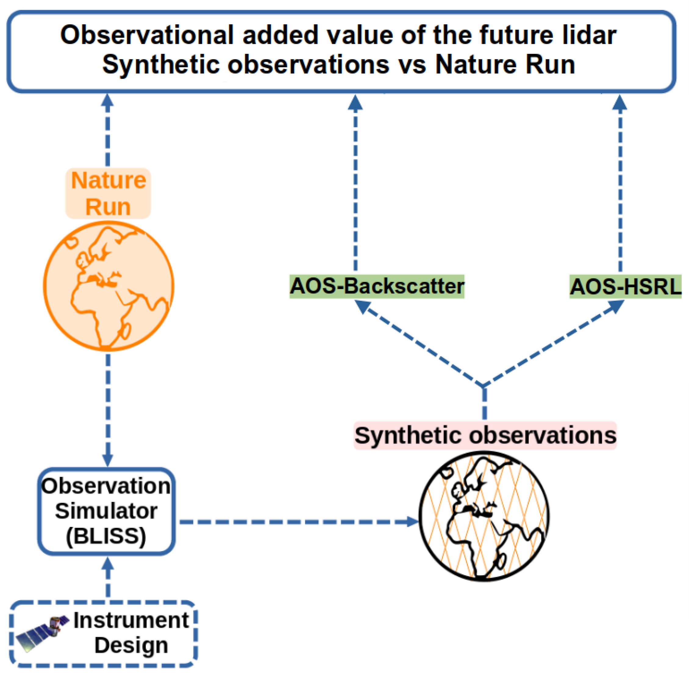
2.1. Method

The first step of this experiment consists of modeling and validating the NR. This atmosphere is expected to be sufficiently realistic for describing the events selected for this study in terms of aerosol abundance and chemical composition, and the respective aerosol optical properties (backscattering and extinction). In particular, the NR must have good correspondence in terms of LR with the represented species to justify the hypotheses during the simulation of the AOS_Backscatter instrument.

The particle extinction and backscatter profiles are then extracted following a typical trajectory of a spaceborne lidar (we used CALIOP trajectories). These extracted aerosol profiles, meteorological fields, and surface properties are integrated as input into an observation simulator for performing the simulations. In this study, the backscatter lidar signal simulator (BLISS) software developed by the CNES is used. Note that this software was developed in the framework of the AOS mission in order to build the SO of several configurations. The simulator and the simulation setup will be presented later in the dedicated article.

For each event, two sets of simulations were performed: one with the standard Fernald inversion method with AOS architecture (altitude, emitted power, etc.…), called AOS_Backscatter, and a second one with the HSRL method, called AOS_HSRL. The SO are then compared to each other and to the NR to access the added value of the HSRL channel for a spaceborne lidar. In the first time, the evaluations are made for each event on a single transect in order to visualize the temporal evolution of the observations along the trajectory. In the second step, a statistical analysis over 5 days from 20 March 2018 to 25 March 2018 (∼20 orbits, ∼1700 profiles at $0.5°\times 0.5°$ resolution) was then performed for the specific case of the desert event. The experiment is schematized in Figure 1.

2.2. The Nature Run

The NR was constructed by assimilating the MODIS (moderate resolution imaging spectroradiometer, [19]) aerosol optical depth (AOD) data at 550 nm with a variational method in the MOCAGE CTM [20]. The period of simulation extended from January to September 2018 where the month of January was considered the spin-up. The meteorological forecast was performed with ARPEGE (Action de Recherche Petite Echelle Grande Echelle) at a six-hour temporal resolution [21].

2.2.1. The MOCAGE Chemistry Transport Model

MOCAGE is an offline 3D CTM developed by Météo-France that provides the chemical state of the atmosphere at a time $\mathrm{t}+\Delta \mathrm{t}$ based on its initial state (atmospheric composition at the time (t)), meteorological inputs, and emission data.

• Meteorological inputs: MOCAGE, being an offline model, receives its meteorological fields from an independent weather model every 3 or 6 h. The fields generally come from the IFS model, the ARPEGE model, ERA-INTERIM [22], or more recently, ERA5 [23] reanalyses.
• Atmospheric composition: MOCAGE describes the chemical composition of the atmosphere on 47 vertical levels from the surface up to 5 hPa, with a resolution of 40 to 800 m at the top of the stratosphere. The horizontal resolution can vary from a local scale ($0.1°\times 0.1°$) to a regional ($0.5°\times 0.5°$) up to the global domain with 1 or 2°. The model was initially developed for gaseous species (112 species implemented), whose processes and interactions are described in [24]. The primary aerosols (PA) were implemented by [25] for four species: desert dust, sea salts (SS), and black and organic carbons (BC, OC). Their descriptions were improved by [26], particularly in the description of deposits, and with the development of the aerosols DAS. The inorganic aerosols were implemented by [27], namely nitrates, sulfates, and ammonium. The large-scale transport, which corresponds to the atmospheric circulation (advection) was calculated thanks to the meteorological fields. Then, the finer resolution processes (convection, turbulent diffusion) were solved from sub-mesh parameterizations (more details in [28]).
• Emissions: Emissions are the sources of pollutants in the atmosphere. They can be determined by emission inventories (anthropogenic, biogenic sources…), or by dynamic emissions for some particles pulled from the surface following a natural forecast (DD, SS). The main emission inventories are MACC-City [29] for anthropogenic pollutants, MEGAN-MACC [30] for biogenic emissions and methane, or GEIA for NOx [31]. The dynamic emissions were calculated with parametrizations via the meteorological parameters listed above. These parametrizations take into account the surface properties (composition, roughness…) and determine the necessary conditions (in general wind force and direction) to pull out a calculated quantity of particles.

In addition to these three elementary inputs, the model equations can be constrained from observations via the MOCAGE-Valentina DAS [32,33] validated for the assimilation of aerosol observations from the imager, such as MODIS [34] and lidar instruments [35]. This technique aims to combine the high spatial and temporal resolutions of the model with good accuracy and specific coverage of the observations.

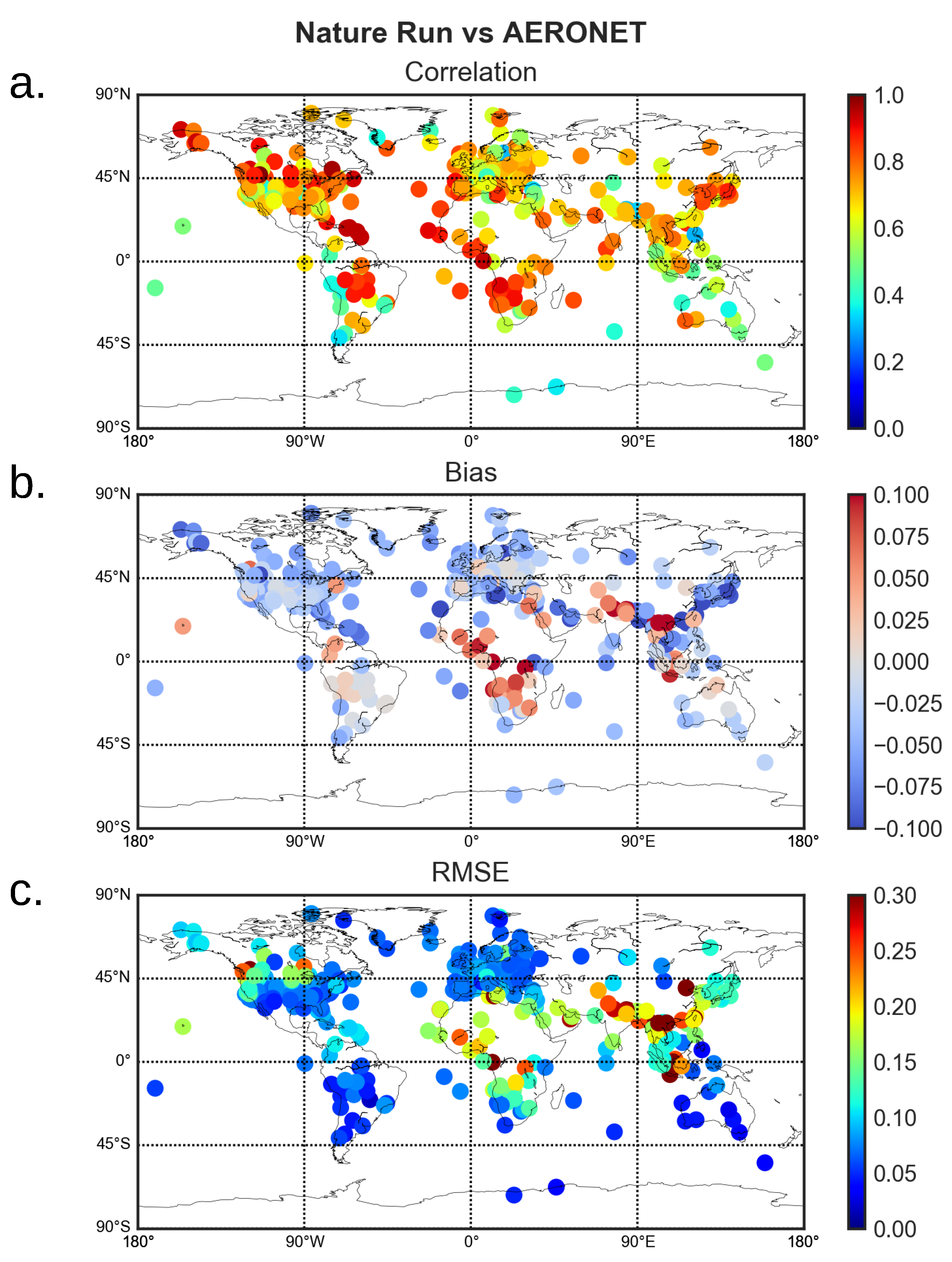
2.2.2. Comparison of the NR with AERONET In Situ Observations

To ensure that the NR is a good representation of reality, we performed a comparative analysis in terms of AOD from the global AErosol RObotic NERwork (AERONET) in situ observations. The aim of this AOD comparison was to check that the total aerosol spatial distribution in the model was realistic in terms of spatial extent, intensity, and variability. However, it should be noted that although the AOD is a good indicator of the total aerosol loading, it is not necessarily representative of the chemical composition of the aerosol species in the atmosphere. AERONET represents hundreds of ground-based sun photometer networks, monitoring optical properties of aerosols from 340 to 1020 nm. With a large spatial coverage and an accuracy of $\pm 0.01$ for AOD at 550 nm, it aims to validate CTM and satellite products for the aerosol study [36]. We used level 1.5 data on version 3 (https://aeronet.gsfc.nasa.gov, last check: 30 November 2022), with automatic cloud screening. Over the globe and for the simulated period of the NR, AERONET provides more than two million measurements with hourly resolution.

This validation has already been performed in the work on the validation of the MODIS pre-operational AOD assimilation system in MOCAGE by El Amraoui et al. (2022), which will serve as a reference for this study. In this reference study, the comparison with AERONET showed that for the year 2018 (the year of the NR) there were relatively low biases and a root mean square error (RMSE) with the exception of Central Africa and South East Asia. These regions are frequently affected by biomass fires and anthropogenic pollution episodes, respectively, phenomena that are sometimes difficult to represent in the model. However, even in these regions, the correlations are satisfactory with values above 0.7. For the years 2018 (2019), average scores of reference for correlation, bias, and root mean square error (RMSE), there were about 0.781 (0.812), −0.01 (−0.007), and 0.128 (0.138), respectively.

For the current study, Figure 2 presents the spatial validation of the NR in terms of correlation, bias, and RMSE at the global scale over the whole simulation period of the NR. The first thing we observe is the good quality of the model on all the statistics in the Europe/Mediterranean and USA/Canada regions, where two of the three events analyzed in this study are located. Concerning the anthropogenic pollution event, this one is located in China and it is not well covered by the AERONET network. The lower scores in terms of bias and RMSE in this region (greater than 0.1 and 0.3, respectively) are accompanied by a good correlation.

Figure 3 completes it with a scatter plot representing the set of AERONET observations in comparison with the NR. The average scores of correlation, bias, and RMSE are about (differences with the 2018 reference) 0.781 (=), 0.026 (+0.036), and 0.138 (+0.01). These differences are of the same order of magnitude as the differences between the references for 2018 and 2019, demonstrating the validity of the NR. We see a positive bias between MODIS assimilation and AERONET stations, strongly driven by the lower (more frequent) AOD values (lower than 0.2). The overestimation of the MODIS observations compared to AERONET in terms of AOD has already been documented in continental surfaces (e.g., [37]) for both the Aqua and Terra platforms. The main differences (in terms of statistics) between the NR and the reference can be attributed to the duration of the simulation, which is shorter in the case of the NR, as well as to the initial state.

2.3. Inversion of the Aerosol Extinction and Backscatter Coefficients

2.3.1. The Lidar Equation

The backscatter coefficients $\beta ({\mathrm{m}}^{-1}·{\mathrm{sr}}^{-1})$ of scatterers (such as particles and molecules) indicate the proportion of light scattered in the opposite direction of the incident photons. On the other hand, the extinction coefficient $\alpha \left({\mathrm{m}}^{-1}\right)$ represents the proportion of light absorbed or scattered in all directions of the volume. These coefficients are key variables in the lidar equation, which connects the backscattered light power ${\mathrm{P}}_{\mathrm{tot}}$ at the range r (directly linked with altitude z as $\mathrm{r}={\mathrm{z}}_{\mathrm{sat}}-\mathrm{z}$ for nadir pointing) for a fixed wavelength $\lambda$ to the optical properties of the atmosphere. In its semi-complete version, this equation can be written as follows:

$${\mathrm{P}}_{\mathrm{tot}}\left(\mathrm{r}\right)=\frac{1}{r^2}\mathrm{K}·\mathrm{G}\left(\mathrm{r}\right)·\left[{\beta }_{\mathrm{m}}\left(\mathrm{r}\right)+{\beta }_{\mathrm{p}}\left(\mathrm{r}\right)\right]·\exp \left[-2{\int }_0^r\left({\alpha }_{\mathrm{m}}\left(\mathrm{r}\right)+\eta {\alpha }_{\mathrm{p}}\left(\mathrm{r}\right)\right)\mathrm{dr}\right]$$

(1)

K and G(r) are related, respectively, to the instrument calibration and to its geometry, and the overlap function between the laser beam and the telescope field of view, which do not involve intrinsic properties of the atmosphere. The extinction and backscattering coefficients are decomposed according to their molecular (m) and particulate (p) fractions. $\eta$, ranging from 0 to 1, is a term that corresponds to the multiple scattering coefficient e.g., [38,39]. This coefficient modulates the phenomenon of light extinction by taking into account the ability of photons to reflect (several times) on the neighboring aerosols when the density is sufficiently high. We consider, hereafter, only simple scattering ($\eta =1$). If the molecular parameters can be directly derived from meteorological profiles (pressure and temperature), the lidar equation still has two unknowns, which makes it unsolvable. On the other hand, the vertical structure of the atmosphere can directly be studied in qualitative terms using attenuated total backscatter (ATB) profiles (see the equation below). However, this Level 1 (L1) product neither provides quantitative information nor indicators of the chemical composition of the atmosphere, which is necessary for a deep understanding of the interactions between aerosols and the environment.

$$\mathrm{ATB}\left(\mathrm{r}\right)=\frac{\mathrm{S}\left(\mathrm{r}\right)}{\mathrm{K}·\mathrm{G}\left(\mathrm{r}\right)}=\left[{\beta }_{\mathrm{m}}\left(\mathrm{r}\right)+{\beta }_{\mathrm{p}}\left(\mathrm{r}\right)\right]·\exp \left[-2{\int }_0^r\left({\alpha }_{\mathrm{m}}\left(\mathrm{r}\right)+{\alpha }_{\mathrm{p}}\left(\mathrm{r}\right)\right)\mathrm{dr}\right]$$

(2)

With $\mathrm{S}\left(\mathrm{r}\right)={\mathrm{r}}^2·{\mathrm{P}}_{\mathrm{tot}}\left(\mathrm{r}\right)$ called the range-corrected lidar signal. For the following steps, the overlap function is assumed to be complete ($\mathrm{G}\left(\mathrm{r}\right)=1$). The aim of this section is to present the two aerosol inversion methods to retrieve the optical properties of the particles compared in this study. The first method is based on the classic inversion algorithm used for elastic backscatter lidar, such as CALIOP, hereafter called the Fernald inversion algorithm. It has the instrumental advantage of requiring a single-simple detection system. However, this method requires a priori assumptions about the state of the atmosphere that can lead to large uncertainties. The second method with high spectral resolution avoids such assumptions by exploiting the Doppler shift phenomenon to separate the molecular component from the total signal. The challenges for both methods are to derive the most accurate distance-dependent particle backscatter, extinction, and lidar ratio profiles ${\mathrm{LR}}_{\mathrm{p}}\left(\mathrm{r}\right)$. This last one is defined as:

$${\mathrm{LR}}_{\mathrm{p}}\left(\mathrm{r}\right)={\alpha }_{\mathrm{p}}\left(\mathrm{r}\right)/{\beta }_{\mathrm{p}}\left(\mathrm{r}\right)$$

(3)

2.3.2. Elastic Backscatter Lidar

The Rayleigh theory assumes a proportional relationship between the extinction and molecular backscatter coefficients of $8\pi /3$, which is not the case for particle coefficients, highly dependent on the shape, size, and chemical compositions of the elements. A first guess of ${\mathrm{LR}}_{\mathrm{p}}$ can, however, be estimated by making an assumption on the observed particulate species, and from empirical measurements of the aerosol properties [40,41,42]. In a parallel way, ${\mathrm{LR}}_{\mathrm{m}}=8\pi /3$ is defined and independent of the range. From the ATB formula, and by replacing the extinction coefficients according to the different lidar ratio and backscatter coefficients, we obtain the following equation:

$$\begin{array}{c}\hfill {\mathrm{LR}}_{\mathrm{p}}\left(\mathrm{r}\right)·\mathrm{ATB}\left(\mathrm{r}\right)·\exp \left[-2{\int }_0^r\left({\mathrm{LR}}_{\mathrm{p}}\left(\mathrm{r}\right)-{\mathrm{LR}}_{\mathrm{m}}\right){\beta }_{\mathrm{m}}\left(\mathrm{r}\right)\mathrm{d}r\right]\\ \hfill =\mathrm{Y}\left(\mathrm{r}\right)·\exp \left[-2{\int }_0^{\mathrm{r}}\mathrm{Y}\left(\mathrm{r}\right)\mathrm{dr}\right]\end{array}$$

(4)

where Y(r) is an introduced term of the form:

$$\mathrm{Y}\left(\mathrm{r}\right)={\mathrm{LR}}_{\mathrm{p}}\left(\mathrm{r}\right)·[{\beta }_{\mathrm{p}}\left(\mathrm{r}\right)+{\beta }_{\mathrm{m}}\left(\mathrm{r}\right)]$$

(5)

At this point, it is reported that all terms on the left-hand side of Equation (4) are known or assumed (i.e., ${\mathrm{LR}}_{\mathrm{p}}$). On the right-hand side, ${\beta }_{\mathrm{p}}$ remains unknown. By putting each member to the logarithm, and applying a derivative with respect to r, we obtain the following equation:

$$\begin{array}{c}\hfill \frac{\mathrm{d}}{\mathrm{d}r}\left[\ln \left(\mathrm{S}\left(\mathrm{r}\right)·{\mathrm{LR}}_{\mathrm{p}}\left(\mathrm{r}\right)·\exp \left[-2{\int }_0^r\left({\mathrm{LR}}_{\mathrm{p}}\left(\mathrm{r}\right)-{\mathrm{LR}}_{\mathrm{m}}\right){\beta }_{\mathrm{m}}\left(\mathrm{r}\right)\mathrm{d}r\right]\right)\right]\\ \hfill =\frac{1}{\mathrm{Y}\left(\mathrm{r}\right)}·\frac{\mathrm{d}\mathrm{Y}\left(\mathrm{r}\right)}{\mathrm{d}r}-2\mathrm{Y}{\left(\mathrm{r}\right)}^2\end{array}$$

(6)

Equation (6) is of the type of Bernoulli’s differential equation, expressed in [43]. The solution is given from the initial condition $\mathrm{Y}\left(r_0\right)={\mathrm{LR}}_{\mathrm{p}}[{\beta }_{\mathrm{p}}\left(r_0\right)+{\beta }_{\mathrm{m}}\left(r_0\right)]$, with $r_0=r_{ref}$, for the retrieval application, where we can consider ${\beta }_{\mathrm{p}}\left(r_0\right)\ll {\beta }_{\mathrm{m}}\left(r_0\right)$ (i.e., an aerosol-free atmosphere). The altitude of reference is often chosen at the top of the troposphere for the wavelength inferior to 700 nm. The total backscatter coefficient profile ${\beta }_{tot}\left(r\right)$ (particular + molecular) is then:

$${\beta }_{tot}\left(\mathrm{r}\right)=\frac{\mathrm{S}\left(\mathrm{r}\right)·\mathrm{Q}\left(\mathrm{r}\right)}{\frac{\mathrm{ATB}\left(r_{ref}\right)}{{\beta }_{}\left(r_{ref}\right)}-2\left({\int }_{r_{ref}}^r{\mathrm{LR}}_{\mathrm{p}}\left({\mathrm{r}}^{\prime }\right)·\mathrm{ATB}\left({\mathrm{r}}^{\prime }\right)·\mathrm{Q}\left({\mathrm{r}}^{\prime }\right){\mathrm{dr}}^{\prime }\right)}$$

(7)

With:

$$\mathrm{Q}\left(x\right)=\exp \left[-2{\int }_{r_{ref}}^x\left({\mathrm{LR}}_{\mathrm{p}}\left(x\right)-{\mathrm{LR}}_{}\right){\beta }_{}\left(x\right)\mathrm{d}x\right]$$

(8)

Finally, we can retrieve first-order solutions of optical coefficients, with an assumption of the lidar ratio fixed independent of the range:

• ${\beta }_{\mathrm{p}}\left(r\right)={\beta }_{tot}\left(r\right)-{\beta }_{}\left(r\right)$
• ${\alpha }_{\mathrm{p}}\left(r\right)={\mathrm{LR}}_{\mathrm{p}}\left(r\right){\beta }_{\mathrm{p}}\left(r\right)$

From this first-order solution, a range-dependant lidar ratio profile can then be determined and implemented in Equations (4) to (8) in a second iteration (or more) to better retrieve the estimated aerosol properties [11,44].

The difficulty of the Fernald inversion method is the definition of the correct LR first guess. As mentioned above, the LR variations depend on the microphysical properties of aerosols, as well as their sizes, shapes, and humidity profiles. For the same family of aerosols, the LR can vary greatly depending on the area of emission. This is the case, for example, for desert dust, with regional variability ranging from 35 to 60 sr [45]. Finally, the LR variability can also be observed along the vertical, either with distinct layers of different particulate species or in homogeneous mixtures. For the same species or a well-mixed layer, the LR can also vary along the vertical via the humidity profile [46]. CALIOP’s LR selection algorithm relies on an aerosol speciation technique based on surface type, layer height, and column-wide-integrated ATB [45]. The algorithm allows for the specification of 11 aerosol species, including 7 in the troposphere. The different LR values for each tropospheric aerosol family are summarized in

Table 1. Empirical LRs for different aerosol species used in the CALIOP inversion algorithm in version 4 at 532 and 1064 nm.

LR (sr)	CM 1	DD	PC 2/S 3	CC 4	PD 5	DM 6	ES 7
532 nm	$23\pm 5$	$44\pm 9$	$70\pm 25$	$53\pm 11$	$55\pm 22$	$37\pm 15$	$70\pm 16$
1064 nm	$23\pm 5$	$44\pm 13$	$30\pm 14$	$30\pm 17$	$48\pm 24$	$37\pm 15$	$30\pm 18$

¹ Clean Marine, ² Polluted Continental, ³ Smoke, ⁴ Clean Continental, ⁵ Polluted Dust, ⁶ Dusty Marine, ⁷ Elevated Smoke.

.

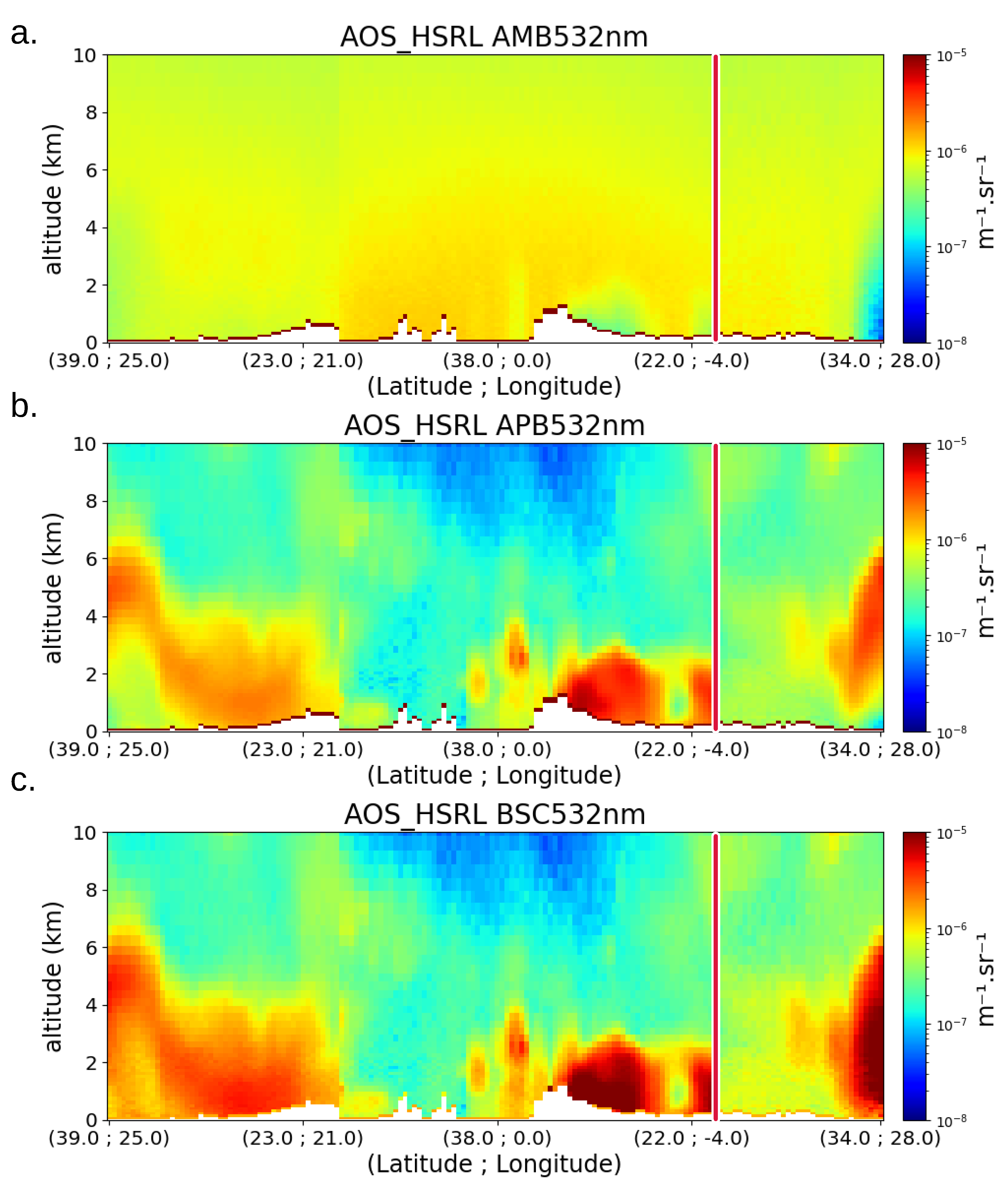
2.3.3. High Spectral Resolution Lidar

In the atmosphere, the scatterers move by random agitation, are responsible for a shift between the incident wavelength and the scattered wavelength (Doppler shift). The signal captured by the detector presents a spectral length larger than the emitted one. The molecules are animated by the Brownian motion characterized by speeds of the order of around $300\mathrm{m}·{\mathrm{s}}^{-1}$, when the agitation of aerosols is mainly driven by wind (around $10\mathrm{m}·{\mathrm{s}}^{-1}$) and turbulence (around $1\mathrm{m}·{\mathrm{s}}^{-1}$). The resulting spectrum clearly shows two distinct diffusion regimes [47]. The first one from particular scattering is very intense and narrow. It is characterized by a frequency shift between 3 and 30 MHz and is most likely similar to the initial spectral length. The second one, more Gaussian, has a width at mid-height of the order of GHz, typical of the Rayleigh regime. By applying a suitable filter, it is possible to discriminate the molecular or particulate fraction of the signal into two different detectors. The Lidar equation of each channel can be formulated as follows, relating to the attenuated molecular backscatter (AMB) or attenuated particular backscatter (APB):

$$\mathrm{AMB}\left(r\right)={\beta }_{\mathrm{m}}\left(r\right)·\exp \left[-2\left({\int }_0^r\left({\alpha }_{\mathrm{m}}\left(r\right)+{\alpha }_{\mathrm{p}}\left(r\right)\right)\mathrm{d}r\right)\right]$$

(9)

$$\mathrm{APB}\left(r\right)={\beta }_{\mathrm{p}}\left(r\right)·\exp \left[-2\left({\int }_0^r\left({\alpha }_{\mathrm{m}}\left(r\right)+{\alpha }_{\mathrm{p}}\left(r\right)\right)\mathrm{d}r\right)\right]$$

(10)

In theory, the determination of the AMB signal and the APB relies on only one laser for deriving the lidar backscatter ratio ${\mathrm{R}}_{\beta }$ (Equation (11)) and then for estimating the backscatter coefficient without any a priori information (Equation (12)). In practice, the determination of the variables is highly dependent on many factors, such as the nature of the filter, its bandwidth, an accurate estimation of the cross-talk between channels, and a good match between the laser frequency and the filter center frequency.

$${\mathrm{R}}_{\beta }\left(r\right)=\frac{\mathrm{AMB}\left(r\right)+\mathrm{APB}\left(r\right)}{\mathrm{AMB}\left(r\right)}$$

(11)

$${\beta }_{\mathrm{p}}\left(r\right)=({\mathrm{R}}_{\beta }\left(r\right)-1)\times {\beta }_{\mathrm{m}}\left(\mathrm{r}\right)$$

(12)

On the other hand, the extinction coefficient is determined from the derivative over the distance of the logarithm of the ratio between the molecular density of the atmosphere ${\mathrm{N}}_{\mathrm{atm}}$ (estimated) and the molecular signal AMB (filtered/measured) (Equation (13)). This estimation is, therefore, more sensitive than the inversion of the backscatter coefficient [48]. Such sensitivity is unfortunate because the extinction determines how much light enters (and is absorbed by) the atmosphere, which is the central key to study the impact of aerosols on the climate.

$${\alpha }_{\mathrm{p}}\left(\mathrm{r}\right)=\frac{1}{2}\frac{\mathrm{d}}{\mathrm{dr}}\left(\ln \left[\frac{{\mathrm{N}}_{\mathrm{atm}}\left(\mathrm{r}\right)}{\mathrm{AMB}\left(\mathrm{r}\right)}\right]\right)-{\alpha }_{\mathrm{m}}\left(\mathrm{r}\right)$$

(13)

Again, these first-order solutions provide distance-dependent lidar Ratio profiles but with much better accuracy. This ${\mathrm{LR}}_{\mathrm{p}}\left(\mathrm{r}\right)$ profile can be injected in turn into Equation (7) to solve the lidar system, as with the previous method. It is worth noting that, in the present study, we focused on the estimation of aerosol backscatter profiles, which have straightforward formulations (Equations (11) and (12)). It does not need the calculation of derivatives of the noisy signal, as is the case for the aerosol extinction profile determination, which is not straightforward and will be tackled in future work.

2.3.4. SO Simulation Setup

BLISS is an end-to-end backscattering lidar simulator developed by the CNES in the framework of the MESCAL (monitoring the evolving state of clouds and aerosol layers) phase 0 (pre-studies for AOS lidar definition). From all of the inputs mentioned, it provides as output the signal received by a backscattering spaceborne lidar (level 0 and level 1 signals, including instrumental noise) and level 2 aerosol and cloud products (particle extinction and backscatter profiles). It simulates lidar instruments with given filter property files using HSRL, or Fernald configuration with a particular LR profile. BLISS is based on the lidar equations as presented in [49] (Chapters 1 to 5). BLISS is modular software. In a simplified way, a first module (scene module) allows for the calculations of the optical coefficients from the definitions of the scenes. A signal module computes the calculation of the optical power from the scene coefficient through the lidar equation and conversion in the electric signal. A third module (L1 Processing) is designed for the determination of the attenuated lidar signal (ATB, AMB, APB…). Finally, the last module (L2 Processing) inverses the optical properties of the scene.

To create the SO, the NR is sampled along a typical trajectory of a satellite lidar instrument, such as CALIOP. The satellite follows a sun-synchronous orbit characterized by an average of two daytime (ascending) and two nighttime (descending) orbits. The solar zenith angle of each scene is computed from the space-time coordinates. The surface properties (roughness and albedo) are determined from the ECOCLIMAP database at a resolution of $1°\times 1°$ (NR resolution). All simulations are made under the assumption of a clear sky without cloud cover (this aspect will be analyzed in future work). The NR atmospheric profiles are extracted in terms of extinction and the particle backscatter at 532 nm from the surface up to ∼14 km in altitude. Observations are averaged with a resolution of $0.5°$ in latitude and longitude and, thus, the horizontal resolution (the distance along which the profiles are averaged) of the SO is fixed to 50 km with a significant impact on the signal-to-noise-ratio (SNR). Since the MOCAGE model does not estimate particle depolarization, we assume that all particles are spherical as a first approximation for estimating their optical properties. Although this is an approximation, the lidar ratios estimated by MOCAGE for non-spherical particles as desert dust are roughly consistent with the literature (see Section 3.1). At the simulator output, the total backscattered lidar power is considered equivalent to the total power detected at the parallel track. The corresponding meteorological profiles (pressure, temperature, and humidity) and the ground altitude are directly taken from CALIOP level 2 (L2) product data, version 4.2 (https://www.icare.univ-lille.fr/; last check: 30 November 2022). All of these inputs are then provided to the BLISS lidar signal simulator together with instrumental parameters from

Table 2. Instrumental characteristics of the CALIOP, AOS_Backscatter, and AOS_HSRL lidar.

Parameter	CALIOP_Like	AOS_Backscatter	AOS_HSRL
Altitude (km)	705	450	450
Wavelength (nm)	532	532	532
Emitted power (W)	2.2	8	8
Pulse duration (ns)	20	15	15
Repetition Frequency (Hz)	20	70	70
Telescope diameter (m)	1	1	1
lidar LOS zenith angle (°)	3	3	3
Filter bandwidth (nm)	0.63	0.1	0.1
HSRL filter	No	No	Yes

for both lidar configurations. As an example, the characteristics of the CALIOP lidar at 532 nm are also noted. The parameters corresponding to the properties of the detectors (e.g., quantum efficiency) are provided with the software and correspond to the characteristics of a photomultiplier tube (PMT) for CALIOP and a Photonis MicroChannel Plate (MCP-PMT-Photonis, [50]) for the two AOS configurations (indicated for 532 and 355 nm). In addition, the transmission coefficients of the HSRL matrix specific to the interferometer filter correspond to classical properties as envisaged in the AOS project.

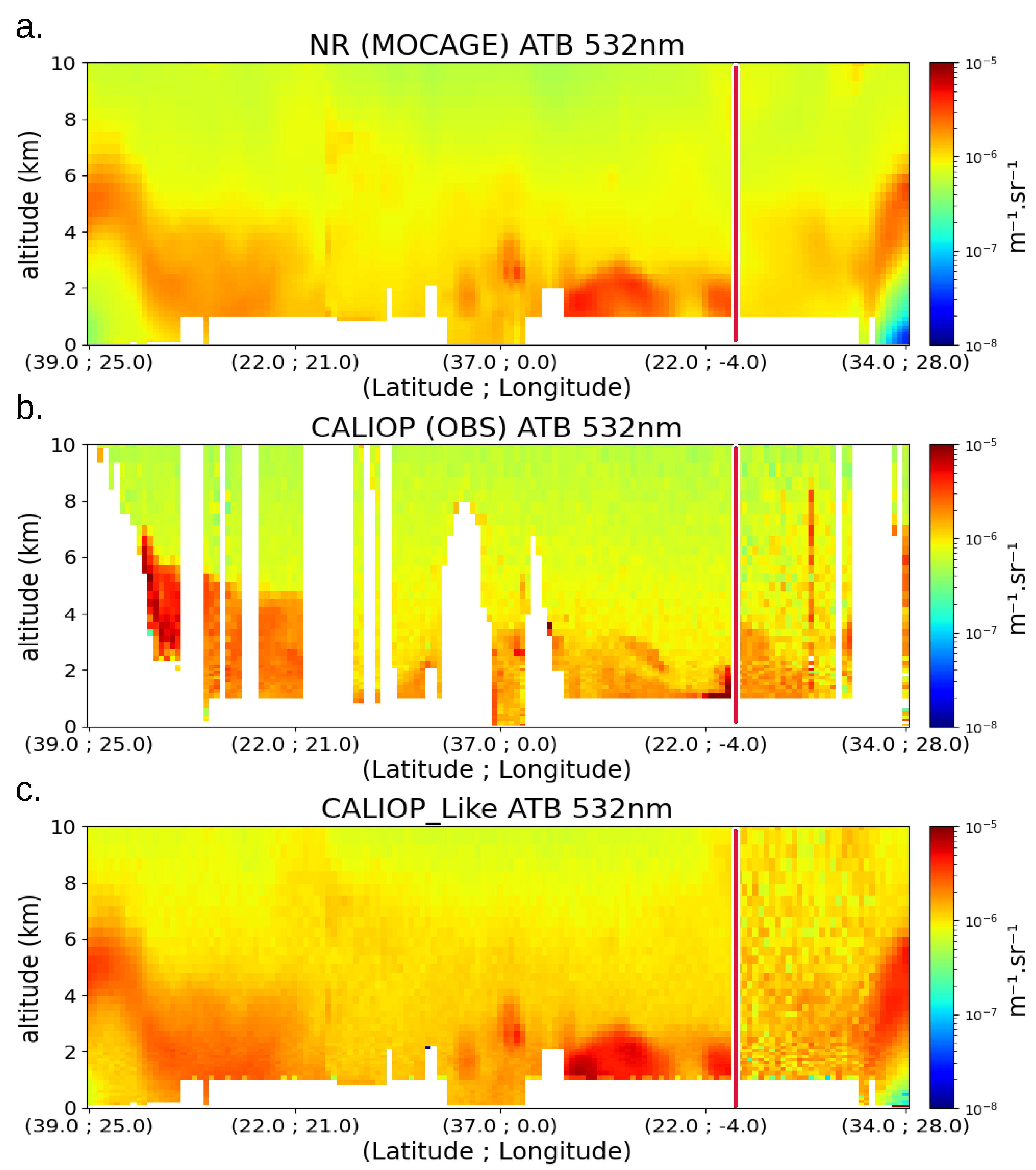
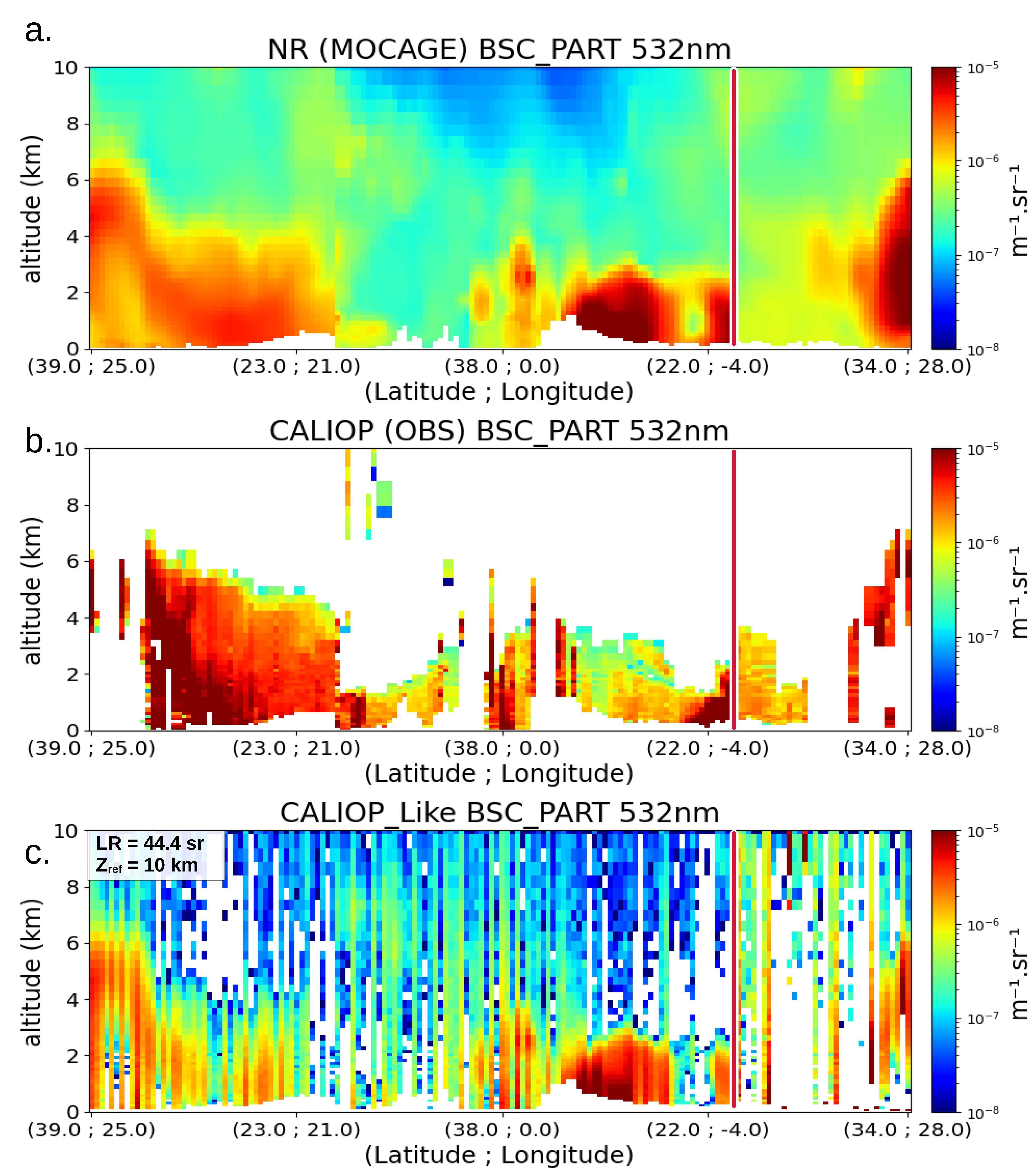
2.3.5. Overview of BLISS Simulation in Comparison with CALIOP Observations

In order to analyze the performance of the BLISS software, this section presents comparisons between the NR, observations from CALIOP (L1, L2), and the equivalent simulation of CALIOP_like synthetic measurements using BLISS with instrumental parameters presented in Table 2 (CALIOP_Like). For this example, we consider a region centered on the Mediterranean Sea, southern Europe, and northern Africa (Medit). This region is bounded by latitudes [50; 20]°$\mathrm{N}$ and longitudes [−20; 40]°$\mathrm{E}$. It corresponds to a desert dust event that occurred on 22 March 2018. The area of analysis is limited to that affected by this event so as to assume an ${\mathrm{LR}}_{\mathrm{p}}=44.4\mathrm{sr}$ as the first guess, which is used as the input of the simulator for desert dust L2 Fernald inversion (Table 1).

First, Figure 4 focuses on the observations (real and synthetic) of ATB at 532 nm. The figure is divided into three ATB transects that follow the CALIOP trajectory. The transect Figure 4a represents the ATB profiles calculated by MOCAGE (implemented by [51]). Blanks (no value) near the surface correspond to the orography. Several aerosol layers can be seen here, some of which can reach 8000 m in altitude and cover large distances. Each aerosol layer is present in the transect Figure 4b, representing the ATB observations of CALIOP. While the intensities in terms of attenuated backscatter may moderately differ, the vertical and horizontal extents of the aerosol layers depicted in the MOCAGE NR are similar to those shown by CALIOP real observations. In the CALIOP real transect, missing data above 1000 m mainly correspond to the presence of opaque clouds, which are not simulated by the MOCAGE setup used here. Figure 4c represents the same transect but for the SO from BLISS.

In both real and synthetic observation transects, we observe a transition from relatively low noise conditions to noisy signals (marked with the red line) and with similar variability associated with noise in both cases. This phenomenon corresponds to the transition between night and daytime measurements, where background sunlight is a source of instrumental noise. This shows that the noise simulated in CALIOP_Like is rather realistic both during the day and night. This difference in noise intensity suggests that we expect a difference in terms of errors and possible divergence in the inverted particle backscatter profiles in the two cases.

Figure 5 is constructed in the same way as Figure 4 but represents the particle backscatter coefficient at 532 nm (obtained from the Fernald inversion in the case of CALIOP and CALIOP_Like transects in panels b and c). The reference altitude set at 10 km shows the best compromise in terms of limited instrumental noise (it is more intense above) and relatively low background aerosol content in the NR (it is more abundant below). Some apparent differences between the NR background abundances of aerosols at the free troposphere may come from the overestimation in the model (Figure 5c) and also partly miss detection in CALIOP measurements (Figure 5b) due to the presence of instrumental noise. This likely occurs between 21°E and 4°W above 5 km of altitude. Note that the resolutions of the L1 and L2 products are not identical (respectively 70 m and 5 km), as well as the estimation of the ground height. The transects Figure 5a–c of ${\beta }_{\mathrm{p}}$ correspond to the NR, the CALIOP observation, and the SO, respectively. As discussed in the previous sections, the inversion of the lidar signal by the Fernald method relies on strong assumptions that can lead to large uncertainties. In agreement with the figure representing the ATB transects and with the literature, Figure 5b shows a significant number of missing or diverging values. The comparison between Figure 5b and Figure 5c must be done with great care. First, the choice of CALIOP LR is based on a selection algorithm, which relies on the integrated measurement of ATB, surface properties, and depolarization (among others). In the case of transect Figure 5c, the first guess is set to 44.4 sr. In addition, the reference altitude is also fixed in the case of the SO transect, at 10 km. At this altitude, we can see that the particle signal is clearly not zero and may correspond to particles of a species other than desert dust.

The retrieved particular backscatter structures shown by CALIOP and CALIOP_Like differ more than in the case of ATB. However, the main structures of desert dust layers are similarly depicted in real and synthetic measurements, especially in terms of the horizontal extent and maximum altitude.

Figure 6 represents the transects of AMB (Figure 6a), APB (Figure 6b), and particular backscatter coefficients (Figure 6c) at 532 nm for the same period as in Figure 4 but with the AOS_HSRL configuration. The brown line at the surface corresponds to the simulated ground echo. The simulated noise is mostly visible for AMB or APB when the signal is under ${10}^{-7}{\mathrm{m}}^{-1}·{\mathrm{sr}}^{-1}$. The impact of sunlight on SNR is less visible than on the CALIOP_Like configuration. This could be attributed to the different altitudes of the satellite, the emitted power of the laser, or the nature of the photodetector, which are parameters with important impacts on the SNR. This improvement in the noise simulation is in accordance with what we expect from a lidar signal simulation. However, the noise levels of AMB and APB are rather low for the transects, leading to good definitions of the inverted particular backscatter profiles.

To conclude this section, the comparisons of ATB transects between NR, CALIOP, and a simulation of CALIOP show good consistency with the BLISS-simulated signals. Simulated noise has the same order of magnitude of in real measurements, both during the day and at night. A systematic overestimation of the simulated signal compared to the NR is calculated to be of the order of [0.5 to 0.2] ${10}^{-6}{\mathrm{m}}^{-1}·{\mathrm{sr}}^{-1}$. The simulated signals compared to the number of measured signals affect the comparison of the level 2 products. The latter shows more deviations from the NR for the Fernald inversions. However, the inverted profiles from measured and simulated signals agree well on average, especially in terms of variability. Therefore, the synthetic observations from BLISS show sufficient consistency so as to apply the same approach to different case studies and lidar configurations.

3. Results

The objective of this section is to illustrate the differences between AOS_Backscatter and AOS_HSRL SO for three case studies corresponding to different events (desert dust, wildfires, and anthropogenic pollution). To account for the dependence of the Fernald inversion method on an a priori LR assumption, each scene focuses on a different aerosol species, which can be associated with one of the tropospheric aerosol families in the CALIOP classification algorithm (see Table 1).

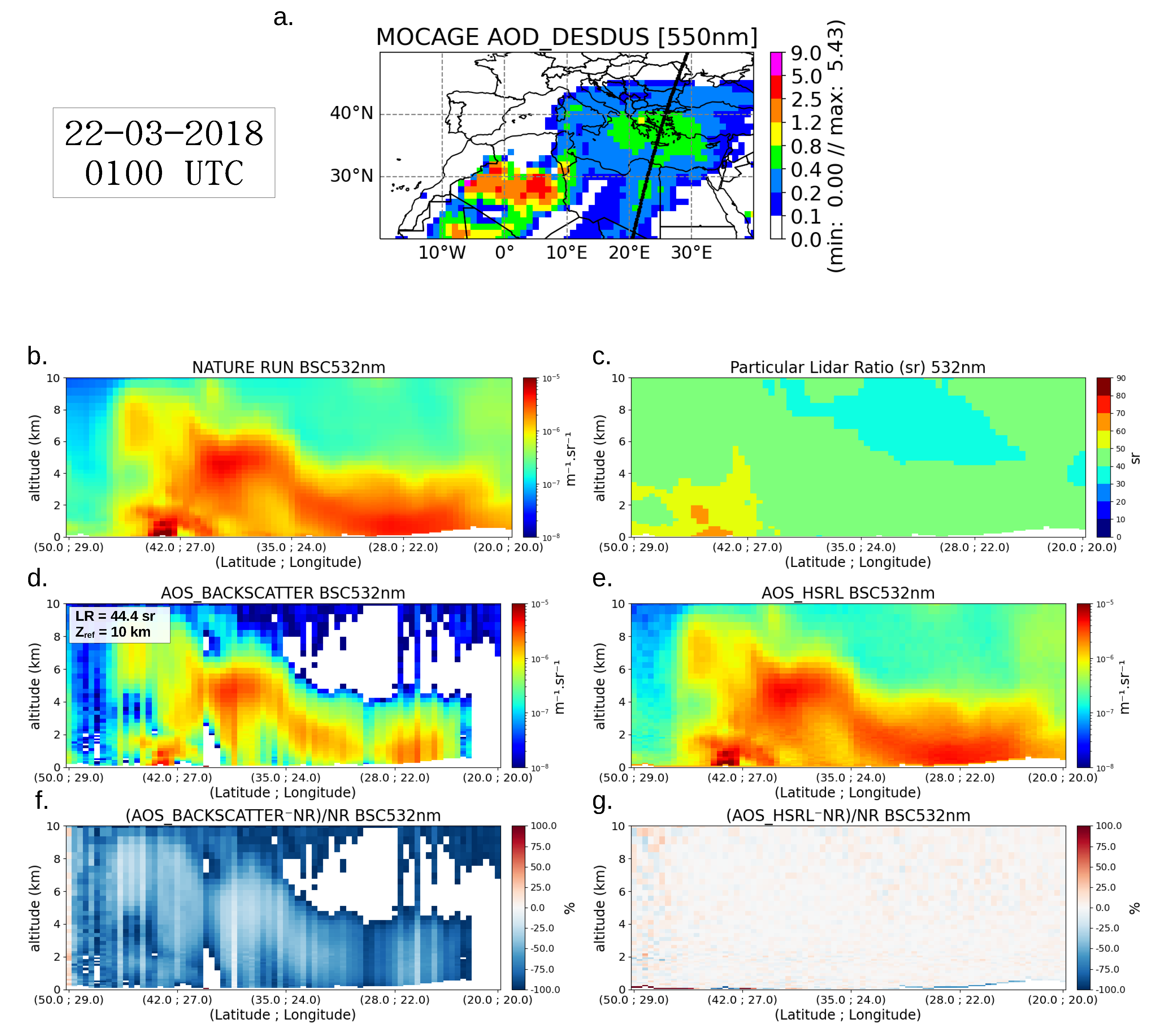
3.1. The Desert Dust Event

Figure 7 shows an example of the added value of an AOS lidar configuration with HSRL compared to a standard (backscatter) configuration for a desert dust event. Figure 7a shows the horizontal distribution of the AOD from the NR corresponding to a desert dust transport event. The thick black line indicates the AOS lidar trajectory from north to south.

Figure 7b represents the transect of the backscatter profiles extracted from the NR following the trajectory of the instrument (the X-axis shows the latitudes and longitudes) as shown in Figure 7a. Figure 7b highlights the plume of the desert dust sampled by the instrument, with high values of the backscatter coefficient and a vertical extent reaching 8000 m at the northernmost point of the plume (latitudes between $\sim 40°\mathrm{N}$ and $\sim 30°\mathrm{N}$).

This plume extends over a fairly large area (latitudes between $\sim 50°\mathrm{N}$ and $\sim 20°\mathrm{N}$) with backscatter coefficients exceeding ${10}^{-5}{\mathrm{m}}^{-1}·{\mathrm{sr}}^{-1}$ and a vertical range of about 4000 m over this region. Figure 7c shows the transects of lidar ratio profiles as estimated in the NR. The variability of the LR is rather limited, especially within the desert dust plume (between 40 and 60 sr). These values of LR are consistent with the assumption of a LR of 44 sr used for the Fernald inversion for this case study. It is also consistent with the LR of desert dust considered in other studies ([52,53]).

Figure 7d shows the transects of particle backscatter coefficient profiles derived from the Fernald inversion (using elastic backscatter lidar measurements, noted as AOS_backscatter). The desert dust plumes depicted by these inverted profiles are consistent with the NR in terms of the overall structures of the plumes and the locations of maximum and minimum values of particle backscatter coefficients. Nevertheless, the inverted particle backscatter profiles are relatively noisy and show significant negative biases. These errors are highlighted in Figure 7f where clear differences between the NR and AOS_backscatter are shown. The large biases (of the order of −80%) are mostly negative for all backscatter profiles. This shows an underestimation of the AOS_backscatter compared to the NR, mainly associated with the assumption of an aerosol-free altitude at 10 km for normalization and differences between the assumed and actual LR.

On the other hand, clearly better performances are found for the particle backscatter profiles derived from the inversions of lidar measurements using HSRL technology (Figure 7e (AOS_HSRL)). This figure shows that the inverted profiles are in very good agreement with the NR profiles, with good localization of the desert dust plume and with almost the same vertical range and particle backscattering values. The difference between AOS_HSRL and NR (Figure 7g) shows that errors in the AOS_HSRL retrieval are random, with very few mean biases. The point-to-point differences between the two datasets oscillate generally between −10 and 15% (it is clearly seen when the color scale of Figure 7g is set to $\pm 30\%$). The results from this figure clearly illustrate the added value of HSRL measurements for a better characterization of the vertical distribution of desert dust aerosol.

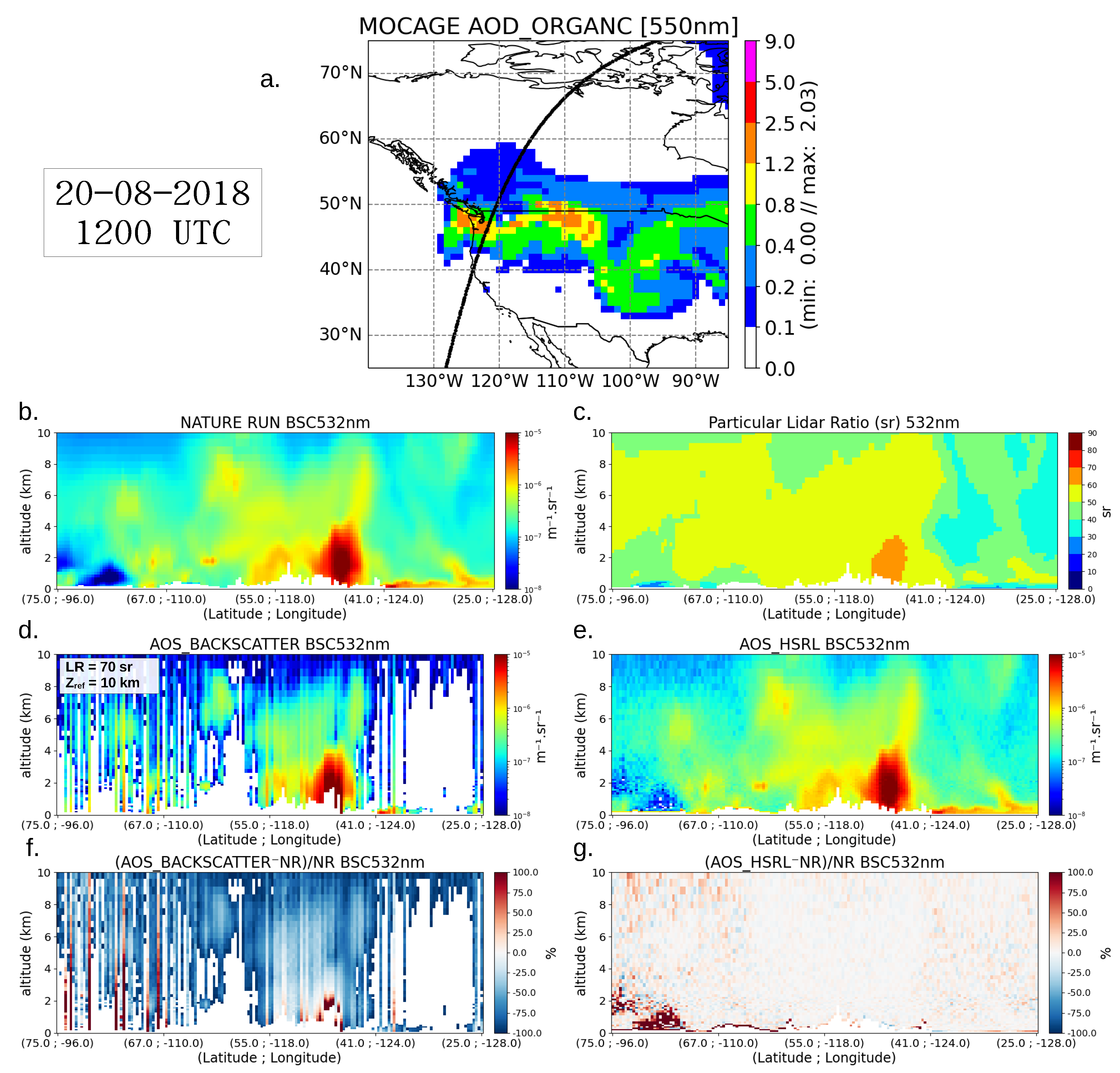
3.2. The Wildfire Event

The second case shown in Figure 8 describes a wildfire event located on the west coast of Canada. The satellite follows a southward trajectory, sampling the thick dense smoke plume at the latitude of $\sim 47°\mathrm{N}$ at 1200 UTC, as can be seen in Figure 8a (in this case, the AOD of organic carbon (OC) is represented). The transects showing the vertical distributions of the smoke layers are seen in Figure 8b, with the densest plume reaching 4000 m. Figure 8c shows the corresponding transect of the lidar ratio, displaying values between 50 and 60 sr over the northern part of the plume (up to a latitude of $\sim 41°\mathrm{N}$) and between 60 and 70 sr at its center. These values are consistent with observations of other biomass-burning events, such as an LR of $70\pm 25$ reported in [45]. We also consider 70 sr as the assumption for the Fernald algorithm for this event, and the reference altitude is set to 10 km.

Around $\sim 40°\mathrm{N}$, the satellite is above the sea surface and no longer observes the smoke plume. This is shown both on the map and on the LR transect where the ratio drops down to 30 sr, far from the uncertainty allowed for the choice of the Fernald assumption in the case of biomass burning. In this area, the most intense layer, close to the surface, is relatively far from the reference altitude.

The result of the AOS_Backscatter lidar inversion shows good retrieval of the vertical structure of the densest part of the smoke plume (errors in AOS_Backscatter of ∼10%, bounded by latitudes [$\sim 55°\mathrm{N}$; $\sim 41°\mathrm{N}$]. The maximum altitude of this part of the plume is about 4000 m. Secondary smoke plumes are also identified, although their particle backscatter coefficients are underestimated and significant errors are apparent. A characteristic artifact of the Fernald inversion can be seen in the center of the plume. The inverted backscatter profiles diverge for large values near the surface, leading to large overestimations or invalid retrievals. This occurs when the denominator of Equation (7) is near zero.

This dense smoke plume around $40°\mathrm{N}$ also shows the lowest errors for AOS_HSRL lidar (between −5% and 5%). The stable and assumption-free HSRL inversion method was not penalized by the high values of particle backscatter coefficients. In contrast with respect to the Fernald-derived profiles, the HSRL approach is capable of observing the whole scene. All secondary smoke plumes are well observed by AOS_HSRL, as well as the thin aerosol plume near the surface over the ocean (with errors between −15% and 15%).

In the case of AOS_HSRL, the retrievals of aerosol backscatter profiles show larger errors over the northern part of the smoke plume (exceeding 40%), and globally, oscillating between −30% and 30% when the backscatter falls below ${10}^{-7}{\mathrm{m}}^{-1}·{\mathrm{sr}}^{-1}$. This phenomenon may be apparent for low particle backscatter conditions and larger instrumental noise [54].

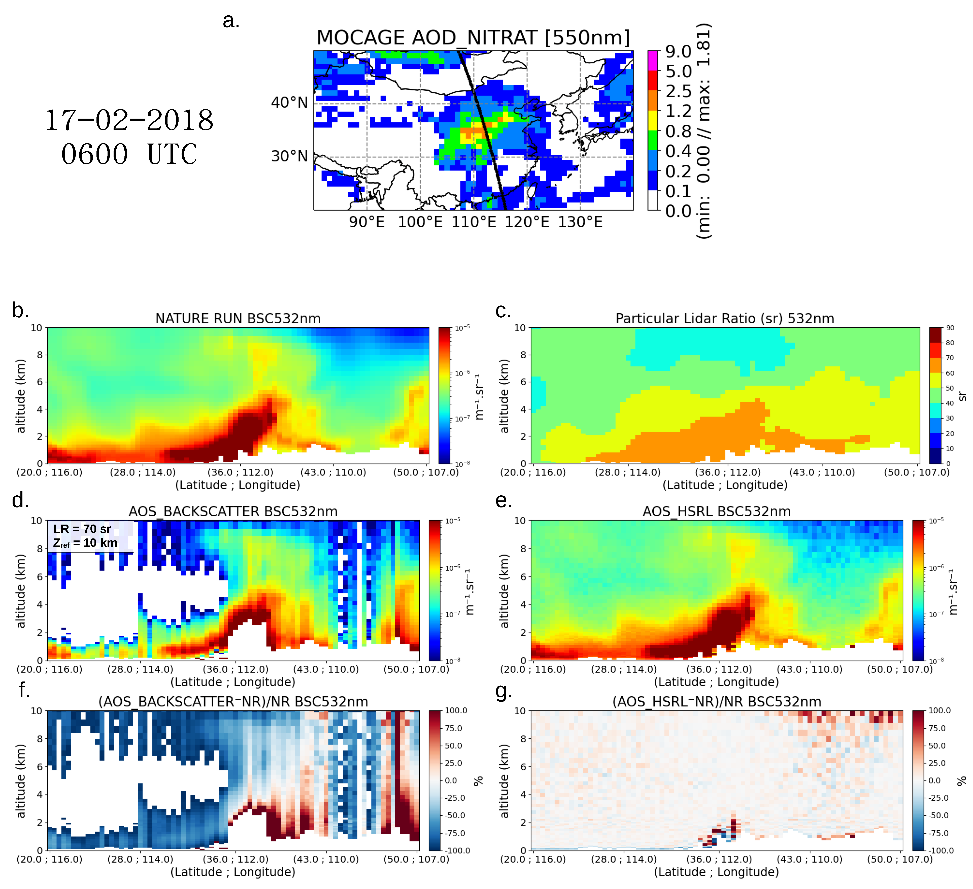
3.3. Urban Pollution Event

The last case concerns a large anthropogenic pollution event over western China (see Figure 9). This region is concerned with frequent anthropogenic pollution episodes in winter in terms of particulate matter of diameters less than $2.5\mathsf{\mu }\mathrm{m}$ (PM2.5) as well as PM10 ${\mathrm{SO}}_2$ and ${\mathrm{NO}}_2$, as reported by [55]. They report 24-h average concentrations of $100\mathsf{\mu }\mathrm{g}·{\mathrm{m}}^{-3}$ (PM2.5), $160\mathsf{\mu }\mathrm{g}·{\mathrm{m}}^{-3}$, (PM10), $40\mathsf{\mu }\mathrm{g}·{\mathrm{m}}^{-3}$ (${\mathrm{SO}}_2$), and $60\mathsf{\mu }\mathrm{g}·{\mathrm{m}}^{-3}$ (${\mathrm{NO}}_2$) averaged in the months of February from 2017 to 2019. Figure 9a effectively highlights a significant nitrate aerosol event (maximum AOS of 1.81) sampled by the satellite at 0600 UTC (ascending orbit). The particle backscatter transect shows a very dense structure at a low altitude (between 0 and ∼2 km), up to ∼6000 m towards $\sim 40°\mathrm{N}$. Up to an average of 5000 m, Figure 9c indicates that the LR is located between 50 and 60 sr with 70 sr for the densest part of the plume. We assume a LR first guess of 70 sr for the polluted continental-type aerosols [45].

Figure 9d clearly depicts saturated Fernald inverted profiles at the lowest parts of the dense aerosol layers (around $36°\mathrm{N}$). This transect is similar to the case study of [56] (in terms of aerosol extinction coefficients), which shows the difficulty of CALIOP to depict the full vertical extent of dense aerosol layers as compared to the airborne HSRL lidar following the same trajectory. Positive saturation at the lowest edge of the aerosol plume can exceed ±150% of relative bias (Figure 9f). This panel also shows the limitations of the inversion method south of the $\sim 36°\mathrm{N}$ latitude from 2000 to 10,000 m up, where the LR of the NR is between 30 and 50 sr. The poor Fernald estimation of the backscatter profile of this region can also be explained by the choice of ${\mathrm{z}}_{\mathrm{ref}}$ at an altitude where the particle backscatter is clearly not zero (∼$5.{10}^7{\mathrm{m}}^{-1}·{\mathrm{sr}}^{-1}$) as compared to the northern latitudes where the inversion is more efficient.

Figure 9e,g show the good ability of the HSRL method to invert all of the aerosol layers as in the two previous cases. In the region where the particle backscatter is greater than ∼${10}^{-7}{\mathrm{m}}^{-1}·{\mathrm{sr}}^{-1}$, the error is around $\pm 5\%$. The relative deviation from the NR exceeds 40% for the points with maximum plume altitudes near the surface, as well as in the region with low particle content for the same reason given in the previous case.

This case summarizes the critical aspect of the good choice of the first guess for the Fernald inversion and the altitude at which the molecular signal is considered to be very large before the particle signal.

3.4. Overall Performance of AOS_Backscatter and AOS_HSRL lidar

To draw a conclusion (with a larger temporal representativity than a single transect), the experiment on the desert dust event was performed over a longer period. The SO were made from 20 to 25 March 2018, a period that covered most of the dust events. This represents ∼20 orbits and ∼1700 profiles at the $0.5°\times 0.5°$ resolution spread over the 5 days of analysis. This episode was selected because atmospheric conditions remain rather stable. Over this region, the variabilities of the LR profiles are rather stable over the whole period, both during the day and at night. This feature limits the contributions of bias during the inversion of elastic backscatter observations. The backscatter profiles are averaged and presented in Figure 10a, as is the NR. The respective standard deviations are presented in Figure 10b. In agreement with the three case studies presented previously, the deviations between NR and AOS_HSRL are very small in comparison with the AOS_Backscatter. Figure 10c represents the relative mean bias (RMB) profiles. Ground echo simulated by BLISS for each profile is removed by not considering the first levels above the surface. The mean bias is estimated at $1.10·{10}^{-10}({\mathrm{m}}^{-1}·{\mathrm{sr}}^{-1})$ (which represents $1.19\%$ of RMB) from ∼500 m up to the maximum altitude of simulation. In contrast, the AOS_Backscatter is characterized by an underestimation of around $-3.53·{10}^{-9}({\mathrm{m}}^{-1}·{\mathrm{sr}}^{-1})$ (which represents ∼−36.13% of RMB), which decreases with the altitude. The shapes of the RMSE profiles in Figure 10d highlight the vertical distribution of errors of the HSRL method, especially at low altitudes (under 4000 m) through more intense plumes. The AOS_HSRL average RMSE is equal to $3.15·{10}^{-7}({\mathrm{m}}^{-1}·{\mathrm{sr}}^{-1})$ under 4000 m, and equal to $1.83·{10}^{-7}({\mathrm{m}}^{-1}·{\mathrm{sr}}^{-1})$ for the whole profile against $2.21·{10}^{-6}({\mathrm{m}}^{-1}·{\mathrm{sr}}^{-1})$, and $1.38·{10}^{-6}({\mathrm{m}}^{-1}·{\mathrm{sr}}^{-1})$ for the AOS_Backscatter SO, respectively.

4. Conclusions

In this study, we analyzed the added value of an HSRL spaceborne lidar with respect to an elastic backscatter lidar, using a lidar signal simulator. The first part of the analysis shows the consistency of the SO, particularly in terms of ATB, as the simulator represents instrumental noise in a similar way as the CALIOP instrument’s real observations (considering different background noise conditions).

We then built two sets of synthetic observations, considering the typical instrumental parameters of the AOS mission, with or without HSRL. We compared the AOS for three study cases, each time representing an orbit in a region centered on a dense aerosol episode. In this way, the uncertainties on the choice of the first guess of the lidar ratio for the classical Fernald inversion of the backscatter lidar measurements were reduced. Each first guess was selected based on the CALIOP inversion algorithm. IRegarding the desert dust plume, with a fairly uniform lidar ratio profile over the observed scene, we were able to study the contribution in terms of the inversion, with relative biases between −5 and +5% for the AOS_HSRL instrument against −80% for the AOS_Backscatter instrument. The biomass burning shows the strong impact of the lidar ratio choice, especially when the satellite sample aerosols were different from smoke, with lower lidar ratios. In this case, the AOS_Backscatter observation diverged and failed to detect the fine structure near the surface. Only the smoke plume was well represented, contrary to AOS_HSRL observations that precisely characterized the whole scene in terms of aerosol backscatter profiles. Finally, the third case study describes an anthropogenic pollution episode, with a well-identified lidar ratio profile over the entire event. This case presents the densest plume in terms of the backscatter coefficient of the three simulated scenes. The AOS_Backscatter instrument fails to invert the base of the aerosol layer. The synthetic observation shows important under- and overestimations exceeding 100%, whereas the AOS_HSRL observation shows good results for the whole event. In terms of relative bias, the HSRL lidar shows its greatest weaknesses when the signal becomes very weak, and the signal-to-noise ratio decreases.

On average, the relative biases between the NR and the various synthetic observations are 1.19% (AOS_HSRL) and −36.13% (AOS_Backscatter). Regarding the RMSE, AOS_HSRL performs on average one order of magnitude better than the AOS_Backscatter compared to NR.

The synthetic observations from AOS_HSRL can then be used to perform an observing simulation system experiment (OSSE) [57] to evaluate the contribution of HSRL satellite lidar products to constrain a transport chemistry model. These types of aerosol OSSE experiments have been mostly performed for passive instruments [58] characterized by good horizontal coverage. Few have been performed for spaceborne aerosol lidar.

This configuration also allows simulating the contribution of a potential UV channel in addition to the visible channel with or without HSRL, to see the added value of such a lidar for different aerosol species.

References

1. WHO. Ambient Air Pollution: A Global Assessment of Exposure and Burden of Disease; World Health Organization: Geneva, Switzerland, 2016; p. 121.
2. Yu, H.; Chin, M.; Yuan, T.; Bian, H.; Remer, L.A.; Prospero, J.M.; Omar, A.; Winker, D.; Yang, Y.; Zhang, Y.; et al. The fertilizing role of African dust in the Amazon rainforest: A first multiyear assessment based on data from Cloud-Aerosol Lidar and Infrared Pathfinder Satellite Observations. Geophys. Res. Lett. 2015, 42, 1984–1991. [Google Scholar] [CrossRef]
3. Boucher, O.; Randall, D.; Artaxo, P.; Bretherton, C.; Feingold, G.; Forster, P.; Kerminen, V.M.; Kondo, Y.; Liao, H.; Lohmann, U.; et al. Clouds and aerosols. In Climate Change 2013: The Physical Science Basis. Contribution of Working Group I to the Fifth Assessment Report of the Intergovernmental Panel on Climate Change; Cambridge University Press: Cambridge, UK, 2013; pp. 571–657. [Google Scholar]
4. Suzuki, K.; Takemura, T. Perturbations to Global Energy Budget Due to Absorbing and Scattering Aerosols. J. Geophys. Res. Atmos. 2019, 124, 2194–2209. [Google Scholar] [CrossRef]
5. Keil, A.; Haywood, J.M. Solar radiative forcing by biomass burning aerosol particles during SAFARI 2000: A case study based on measured aerosol and cloud properties. J. Geophys. Res. Atmos. 2003, 108, SAF3-1. [Google Scholar] [CrossRef]
6. Su, T.; Li, Z.; Li, C.; Li, J.; Han, W.; Shen, C.; Tan, W.; Wei, J.; Guo, J. The significant impact of aerosol vertical structure on lower atmosphere stability and its critical role in aerosol–planetary boundary layer (PBL) interactions. Atmos. Chem. Phys. 2020, 20, 3713–3724. [Google Scholar] [CrossRef] [Green Version]
7. Ch, D.; Wood, R.; Anderson, T.L.; Satheesh, S.K.; Charlson, R.J. Satellite-derived direct radiative effect of aerosols dependent on cloud cover. Nat. Geosci 2009, 2, 181–184. [Google Scholar] [CrossRef]
8. Winker, D.M.; Vaughan, M.A.; Omar, A.; Hu, Y.; Powell, K.A.; Liu, Z.; Hunt, W.H.; Young, S.A. Overview of the CALIPSO Mission and CALIOP Data Processing Algorithms. J. Atmos. Ocean. Technol. 2009, 26, 2310–2323. [Google Scholar] [CrossRef]
9. Winker, D.M.; Tackett, J.L.; Getzewich, B.J.; Liu, Z.; Vaughan, M.A.; Rogers, R.R. The global 3-D distribution of tropospheric aerosols as characterized by CALIOP. Atmos. Chem. Phys. 2013, 13, 3345–3361. [Google Scholar] [CrossRef] [Green Version]
10. Song, Q.; Zhang, Z.; Yu, H.; Ginoux, P.; Shen, J. Global dust optical depth climatology derived from CALIOP and MODIS aerosol retrievals on decadal timescales: Regional and interannual variability. Atmos. Chem. Phys. 2021, 21, 13369–13395. [Google Scholar] [CrossRef]
11. Klett, J.D. Stable analytical inversion solution for processing lidar returns. Appl. Opt. 1981, 20, 211–220. [Google Scholar] [CrossRef] [Green Version]
12. Fernald, F.G.; Herman, B.M.; Reagan, J.A. Determination of Aerosol Height Distributions by Lidar. J. Appl. Meteorol. Climatol. 1972, 11, 482–489. [Google Scholar] [CrossRef]
13. Reitebuch, O.; Lemmerz, C.; Nagel, E.; Paffrath, U.; Durand, Y.; Endemann, M.; Fabre, F.; Chaloupy, M. The Airborne Demonstrator for the Direct-Detection Doppler Wind Lidar ALADIN on ADM-Aeolus. Part I: Instrument Design and Comparison to Satellite Instrument J. Atmos. Ocean. Technol. 2009, 26, 2501–2515. [Google Scholar]
14. Flamant, P.; Cuesta, J.; Denneulin, M.L.; Dabas, A.; Huber, D. ADM-Aeolus retrieval algorithms for aerosol and cloud products. Tellus A Dyn. Meteorol. Oceanogr. 2008, 60, 273–286. [Google Scholar] [CrossRef]
15. Illingworth, A.J.; Barker, H.W.; Beljaars, A.; Ceccaldi, M.; Chepfer, H.; Clerbaux, N.; Cole, J.; Delanoë, J.; Domenech, C.; Donovan, D.P.; et al. The EarthCARE Satellite: The Next Step Forward in Global Measurements of Clouds, Aerosols, Precipitation, and Radiation. Bull. Am. Meteorol. Soc. 2015, 96, 1311–1332. [Google Scholar] [CrossRef] [Green Version]
16. Ansmann, A.; Müller, D. Lidar and Atmospheric Aerosol Particles. In Lidar: Range-Resolved Optical Remote Sensing of the Atmosphere; Weitkamp, K., Ed.; Springer: New York, NY, USA, 2005. [Google Scholar]
17. Braun, S.A.; Yorks, J.; Thorsen, T.; Cecil, D.; Kirschbaum, D. NASA’S Earth System Observatory-Atmosphere Observing System. In Proceedings of the IGARSS 2022—2022 IEEE International Geoscience and Remote Sensing Symposium, Kuala Lumpur, Malaysia, 17–22 July 2022; pp. 7391–7393. [Google Scholar] [CrossRef]
18. Burton, S.; Ferrare, R.; Hostetler, C.; Hair, J.; Rogers, R.; Obland, M.; Butler, C.; Cook, A.; Harper, D.; Froyd, K. Aerosol classification using airborne High Spectral Resolution Lidar measurements–methodology and examples. Atmos. Meas. Tech. 2012, 5, 73–98. [Google Scholar] [CrossRef] [Green Version]
19. King, M.D.; Kaufman, Y.J.; Menzel, W.P.; Tanre, D. Remote sensing of cloud, aerosol, and water vapor properties from the Moderate Resolution Imaging Spectrometer(MODIS). IEEE Trans. Geosci. Remote. Sens. 1992, 30, 2–27. [Google Scholar] [CrossRef] [Green Version]
20. El Amraoui, L.; Plu, M.; Guidard, V.; Cornut, F.; Bacles, M. A Pre-Operational System Based on the Assimilation of MODIS Aerosol Optical Depth in the MOCAGE Chemical Transport Model. Remote. Sens. 2022, 14, 1949. [Google Scholar] [CrossRef]
21. Courtier, P.; Freydier, C.; Geleyn, J.; Rabier, F.; Rochas, M. The ARPEGE project at Météo France. In Proceedings of the Atmospheric Models, Workshop on Numerical Methods, Shinfield Park, Reading, UK, 9–13 September 1991; ECMWF. Volume 2, pp. 193–231. Available online: https://www.ecmwf.int/en/elibrary/74049-arpege-project-meteo-france (accessed on 8 December 2022).
22. Dee, D.P.; Uppala, S.M.; Simmons, A.J.; Berrisford, P.; Poli, P.; Kobayashi, S.; Andrae, U.; Balmaseda, M.A.; Balsamo, G.; Bauer, P.; et al. The ERA-Interim reanalysis: Configuration and performance of the data assimilation system. Q. J. R. Meteorol. Soc. 2011, 137, 553–597. [Google Scholar] [CrossRef]
23. Hersbach, H.; Bell, B.; Berrisford, P.; Hirahara, S.; Horányi, A.; Muñoz-Sabater, J.; Nicolas, J.; Peubey, C.; Radu, R.; Schepers, D.; et al. The ERA5 global reanalysis. Q. J. R. Meteorol. Soc. 2020, 146, 1999–2049. [Google Scholar] [CrossRef]
24. Cussac, M. La Composition Chimique de la Haute Troposphère: éTude de l’impact des Feux de Biomasse et des Processus de Transports Verticaux Avec le Modèle MOCAGE et les Mesures IAGOS; Institut National Polytechnique de Toulouse: Toulouse, France, 2020; Available online: https://www.theses.fr/2020INPT0128 (accessed on 8 December 2022).
25. Martet, M.; Peuch, V.H.; Laurent, B.; Marticorena, B.; Bergametti, G. Evaluation of long-range transport and deposition of desert dust with the CTM MOCAGE. Tellus B 2009, 61, 449–463. [Google Scholar] [CrossRef]
26. Sič, B.; El Amraoui, L.; Marécal, V.; Josse, B.; Arteta, J.; Guth, J.; Joly, M.; Hamer, P. Modelling of primary aerosols in the chemical transport model MOCAGE: Development and evaluation of aerosol physical parameterizations. Geosci. Model Dev. 2015, 8, 381–408. [Google Scholar] [CrossRef]
27. Guth, J.; Josse, B.; Marécal, V.; Joly, M.; Hamer, P. First implementation of secondary inorganic aerosols in the MOCAGE version R2.15.0 chemistry transport model. Geosci. Model Dev. 2016, 9, 137–160. [Google Scholar] [CrossRef] [Green Version]
28. Josse, B.; Simon, P.; Peuch, V.H. Radon global simulation with the multiscale chemistry trasnport model MOCAGE. Tellus 2004, 56, 339–356. [Google Scholar] [CrossRef]
29. Lamarque, J.F.; Bond, T.C.; Eyring, V.; Granier, C.; Heil, A.; Klimont, Z.; Lee, D.; Liousse, C.; Mieville, A.; Owen, B.; et al. Historical (1850–2000) gridded anthropogenic and biomass burning emissions of reactive gases and aerosols: Methodology and application. Atmos. Chem. Phys. 2010, 10, 7017–7039. [Google Scholar] [CrossRef] [Green Version]
30. Sindelarova, K.; Granier, C.; Bouarar, I.; Guenther, A.; Tilmes, S.; Stavrakou, T.; Müller, J.F.; Kuhn, U.; Stefani, P.; Knorr, W. Global data set of biogenic VOC emissions calculated by the MEGAN model over the last 30 years. Atmos. Chem. Phys. 2014, 14, 9317–9341. [Google Scholar] [CrossRef] [Green Version]
31. Yienger, J.J.; Levy II, H. Empirical model of global soil-biogenic NOx emissions. J. Geophys. Res. Atmos. 1995, 100, 11447–11464. [Google Scholar] [CrossRef]
32. Emili, E.; Barret, B.; Massart, S.; Le Flochmoen, E.; Piacentini, A.; El Amraoui, L.; Pannekoucke, O.; Cariolle, D. Combined assimilation of IASI and MLS observations to constrain tropospheric and stratospheric ozone in a global chemical transport model. Atmos. Chem. Phys. 2014, 14, 177–198. [Google Scholar] [CrossRef] [Green Version]
33. El Amraoui, L.; Attié, J.L.; Ricaud, P.; Lahoz, W.A.; Piacentini, A.; Peuch, V.H.; Warner, J.X.; Abida, R.; Barré, J.; Zbinden, R. Tropospheric CO vertical profiles deduced from total columns using data assimilation: Methodology and Validation. Atmos. Meas. Tech. 2014, 7, 3035–3057. [Google Scholar] [CrossRef] [Green Version]
34. Sič, B.; El Amraoui, L.; Piacentini, A.; Marécal, V.; Emili, E.; Cariolle, D.; Prather, M.; Attié, J.L. Aerosol data assimilation in the chemical transport model MOCAGE during the TRAQA/ChArMEx campaign: Aerosol optical depth. Atmos. Meas. Tech. 2016, 9, 5535–5554. [Google Scholar] [CrossRef] [Green Version]
35. El Amraoui, L.; Sič, B.; Piacentini, A.; Marécal, V.; Frebourg, N.; Attié, J.L. Aerosol data assimilation in the MOCAGE chemical transport model during the TRAQA/ChArMEx campaign: Lidar observations. Atmos. Meas. Tech. 2020, 13, 4645–4667. [Google Scholar] [CrossRef]
36. Holben, B.; Eck, T.; Slutsker, I.; Tanre, D.; Buis, J.; Setzer, A.; Vermote, E.; Reagan, J.; Kaufman, Y.; Nakajima, T.; et al. AERONET—A federated instrument network and data archive for aerosol characterization. Remote. Sens. Environ. 1998, 66, 1–16. [Google Scholar] [CrossRef]
37. Royer, P.; Raut, J.C.; Ajello, G.; Berthier, S.; Chazette, P. Synergy between CALIOP and MODIS instruments for aerosol monitoring: Application to the Po Valley. Atmos. Meas. Tech. 2010, 3, 893–907. [Google Scholar] [CrossRef] [Green Version]
38. Young, S.; Winker, D.; Vaughan, M.; Hu, Y.; Kuehn, R. Extinction Retrieval Algorithms, CALIOP Algorithm Theoretical Basis Document PC-SCI-202 Part 4. 2008. Available online: http://www-calipso.larc.nasa.gov/resources/pdfs/PC-SCI-202Part4v1.0.pdf (accessed on 8 December 2022).
39. Cuesta, J.; Marsham, J.; Parker, D.; Flamant, C. Dynamical mechanisms controlling the vertical redistribution of dust and the thermodynamic structure of the West Saharan Atmospheric Boundary Layer during Summer. Atmos. Sci. Lett. 2009, 10, 34–42. [Google Scholar] [CrossRef]
40. Papagiannopoulos, N.; Mona, L.; Alados-Arboledas, L.; Amiridis, V.; Baars, H.; Binietoglou, I.; Bortoli, D.; D’Amico, G.; Giunta, A.; Guerrero-Rascado, J.L.; et al. CALIPSO climatological products: Evaluation and suggestions from EARLINET. Atmos. Chem. Phys. 2016, 16, 2341–2357. [Google Scholar] [CrossRef] [Green Version]
41. Liu, Z.; Winker, D.; Omar, A.; Vaughan, M.; Kar, J.; Trepte, C.; Hu, Y.; Schuster, G. Evaluation of CALIOP 532 nm aerosol optical depth over opaque water clouds. Atmos. Chem. Phys. 2015, 15, 1265–1288. [Google Scholar] [CrossRef] [Green Version]
42. Omar, A.; Liu, Z.; Vaughan, M.; Thornhill, K.; Kittaka, C.; Ismail, S.; Hu, Y.; Chen, G.; Powell, K.; Winker, D.; et al. Extinction-to-backscatter ratios of Saharan dust layers derived from in situ measurements and CALIPSO overflights during NAMMA. J. Geophys. Res. Atmos. 2010, 115, D24. [Google Scholar] [CrossRef] [Green Version]
43. Sasano, Y.; Browell, E.V.; Ismail, S. Error caused by using a constant extinction/backscattering ratio in the lidar solution. Appl. Opt. 1985, 24, 3929–3932. [Google Scholar] [CrossRef]
44. Klett, J.D. Lidar inversion with variable backscatter/extinction ratios. Appl. Opt. 1985, 24, 1638–1643. [Google Scholar] [CrossRef]
45. Kim, M.H.; Omar, A.H.; Tackett, J.L.; Vaughan, M.A.; Winker, D.M.; Trepte, C.R.; Hu, Y.; Liu, Z.; Poole, L.R.; Pitts, M.C.; et al. The CALIPSO version 4 automated aerosol classification and lidar ratio selection algorithm. Atmos. Meas. Tech. 2018, 11, 6107–6135. [Google Scholar] [CrossRef] [Green Version]
46. Randriamiarisoa, H.; Chazette, P.; Couvert, P.; Sanak, J.; Mégie, G. Relative humidity impact on aerosol parameters in a Paris suburban area. Atmos. Chem. Phys. 2006, 6, 1389–1407. [Google Scholar] [CrossRef] [Green Version]
47. Cheng, Z.; Liu, D.; Yang, Y.; Yang, L.; Huang, H. Interferometric filters for spectral discrimination in high-spectral-resolution lidar: Performance comparisons between Fabry–Perot interferometer and field-widened Michelson interferometer. Appl. Opt. 2013, 52, 7838–7850. [Google Scholar] [CrossRef]
48. Eloranta, E. High Spectral Resolution Lidar. In Lidar: Range-Resolved Optical Remote Sensing of the Atmosphere; Weitkamp, K., Ed.; Springer: New York, NY, USA, 2005. [Google Scholar]
49. Weitkamp, C. Lidar: Range-Resolved Optical Remote Sensing of the Atmosphere; Springer Series in Optical Sciences; Springer: New York, NY, USA, 2005. [Google Scholar] [CrossRef]
50. Orlov, D.A.; Glazenborg, R.; Ortega, R.; Kernen, E. High-detection efficiency MCP-PMTs with single photon counting capability for LIDAR applications. In Proceedings of the International Conference on Space Optics—ICSO, Chania, Greece, 9–12 October 2018; Sodnik, Z., Karafolas, N., Cugny, B., Eds.; International Society for Optics and Photonics, SPIE: Bellingham, WA, USA, 2019; Volume 11180, p. 1118031. [Google Scholar] [CrossRef] [Green Version]
51. Sič, B. Amélioration de la représentation des aérosols dans un modèle de chimie-transport: Modélisation et assimilation de données. Ph.D. Thesis, Université de Toulouse, Université Toulouse III-Paul Sabatier, Toulouse, France, 2014. [Google Scholar]
52. Dong, Q.; Huang, Z.; Li, W.; Li, Z.; Song, X.; Liu, W.; Wang, T.; Bi, J.; Shi, J. Polarization Lidar Measurements of Dust Optical Properties at the Junction of the Taklimakan Desert & ndash;Tibetan Plateau. Remote. Sens. 2022, 14, 558. [Google Scholar] [CrossRef]
53. Han, Y.; Wang, T.; Tang, J.; Wang, C.; Jian, B.; Huang, Z.; Huang, J. New insights into the Asian dust cycle derived from CALIPSO lidar measurements. Remote. Sens. Environ. 2022, 272, 112906. [Google Scholar] [CrossRef]
54. Xiao, D.; Wang, N.; Shen, X.; Landulfo, E.; Zhong, T.; Liu, D. Development of ZJU High-Spectral-Resolution Lidar for Aerosol and Cloud: Extinction Retrieval. Remote. Sens. 2020, 12, 3047. [Google Scholar] [CrossRef]
55. Chen, Q.X.; Huang, C.L.; Yuan, Y.; Tan, H.P. Influence of COVID-19 Event on Air Quality and their Association in Mainland China. Aerosol Air Qual. Res. 2020, 20, 1541–1551. [Google Scholar] [CrossRef]
56. McPherson, C.J.; Reagan, J.A.; Schafer, J.; Giles, D.; Ferrare, R.; Hair, J.; Hostetler, C. AERONET, airborne HSRL, and CALIPSO aerosol retrievals compared and combined: A case study. J. Geophys. Res. Atmos. 2010, 115. [Google Scholar] [CrossRef]
57. Masutani, M.; Schlatter, T.W.; Errico, R.M.; Stoffelen, A.; Andersson, E.; Lahoz, W.; Woollen, J.S.; Emmitt, G.D.; Riishøjgaard, L.P.; Lord, S.J. Observing System Simulation Experiments. In Data Assimilation; Lahoz, W., Khattatov, B., Menard, R., Eds.; Springer: Berlin/Heidelberg, Germany, 2010; pp. 647–679. [Google Scholar] [CrossRef]
58. Timmermans, R.; Segers, A.J.; Builtjes, P.J.; Vautard, R.; Siddans, R.; Elbern, H.; Tjemkes, S.A.; Schaap, M. The added value of a proposed satellite imager for ground level particulate matter analyses and forecasts. IEEE J. Sel. Topics Appl. Earth Obs. Remote Sens. 2009, 2, 271–283. [Google Scholar] [CrossRef]
Figure 1. Schematic representation of the experience principle.
Remotesensing 15 00506 g001
Figure 2. Maps of comparison between the NR and the AERONET of in situ observations in terms of AOD over the globe, from 1 February to 31 September 2018. Statistics are performed in terms of (a): correlation, (b): bias, and (c): RMSE.
Remotesensing 15 00506 g002
Figure 3. Scatter plot of AERONET vs. NR in terms of AOD from 1 February to 31 September 2018.
Remotesensing 15 00506 g003
Figure 4. Comparison of ATB transects at 532 nm along the trajectory of CALIOP for 22 March 2018 over the Medit region. (a) Transect from the NR, (b) CALIOP observations, and (c) the corresponding CALIOP_Like SO. The vertical red line corresponds to the start of the daytime orbit (1229UTC).
Remotesensing 15 00506 g004
Figure 5. Comparison of particular backscatter coefficient transects at 532 nm along the trajectory of CALIOP for 22 March 2018, over the Medit region. (a) Transect from the NR, (b) CALIOP observations, and (c) the corresponding CALIOP_Like SO. The vertical red line corresponds to the start of the daytime orbit (1229UTC).
Remotesensing 15 00506 g005
Figure 6. AOS_Like SO in terms of AMB, APB, and the particular coefficient backscatter at 532 nm along the trajectory of CALIOP for 22 March 2018 over the Medit region. (a) Transect of AMB (b) Transect of APB, and (c) transect of synthetic particular backscatter coefficient. The vertical red line corresponds to the start of the daytime orbit (1229UTC).
Remotesensing 15 00506 g006
Figure 7. Case from 22 March 2018 at 0100 UTC. (a) AOD of DD from the NR together with the studied satellite trajectory (black line). (b) Particular backscatter profile transects of a desert dust outbreak along the satellite trajectory in the NR. (c) Corresponding particular lidar ratio transect calculated from the NR. (d,e) Simulation of the backscatter coefficient SO for the AOS_Backscatter and the AOS_HSRL configurations. (f,g) Relative mean bias (SO-NR)/NR of both instruments.
Remotesensing 15 00506 g007
Figure 8. Case from 20 August 2018 at 1200 UTC. (a) AOD of organic carbon from the NR together with the studied satellite trajectory (black line). (b) Particular backscatter profile transects of biomass burning along the satellite trajectory in the NR. (c) Corresponding particular lidar ratio transect calculated from the NR. (d,e) Simulation of the backscatter coefficient SO for the AOS_Backscatter and the AOS_HSRL configurations. (f,g) Relative mean bias (SO-NR)/NR of both instruments.
Remotesensing 15 00506 g008
Figure 9. Case from 17 March 2018 at 0600 UTC. (a) AOD of nitrate aerosols from the NR together with the studied satellite trajectory (black line). (b) Particular backscatter profile transects of an urban pollution event over China along the satellite trajectory in the NR. (c) Corresponding particular lidar ratio transect calculated from the NR. (d,e) Simulation of the backscatter coefficient SO for the AOS_Backscatter and the AOS_HSRL configurations. (f,g) Relative mean bias (SO-NR)/NR of both instruments.
Remotesensing 15 00506 g009
Figure 10. (a) Average profiles of particular backscatter coefficients at 532 nm from the NR (blue), the AOS_Backscatter SO (orange), and the AOS_HSRL SO (green) from 20 March to 25 March 2018 over the Medit region. (b) Corresponding standard deviation profiles. (c) Relative mean biases (SO-NR)/NR of both instruments. (d) RMSEs of both instruments versus the NR.
Remotesensing 15 00506 g010