Abstract
In the remote sensing monitoring of conservation tillage, the acquisition of remote sensing data with high spatial and temporal resolution is critical. The current optical remote sensing images cannot realize both temporal and spatial resolution, especially under cloud and rain interference. Thus, this study employs the enhanced spatial and temporal adaptive reflectance fusion model (ESTARFM) to obtain the normalized difference tillage index (NDTI) with both temporal and spatial resolution estimated by Sentinel−2 and MODIS using the Index−then−Blend (IB) and Blend−then−Index (BI) fusion schemes. After comparison, the IB scheme was better than the BI scheme in predicting results and prediction efficiency. The NDTI predicted by ESTARFM and Sentinel−2 on June 12, 2020 was compared. A coefficient of determination R2 of 0.73 and RMSE of 0.000117 was obtained, indicating a high prediction accuracy, which meets the prediction requirements. Based on the predicted ESTARFM NDTI of the study area on May 17, 2021, the maize residue cover (MRC) of the study area was estimated using the previously constructed MRC unary linear regression model. The MRC of the sampling points of the remote sensing images was estimated by verifying the predicted ESTARFM NDTI with the MRC of the sampling points taken in the field extracted by the maximum likelihood classifier, which has a coefficient of determination R2 of 0.78 and RMSE of 0.00676, signifying better prediction results. The proposed method provides considerable data sources for the remote sensing monitoring studies of conservation tillage.
1. Introduction
Northeast China is the largest grain−producing region in China and has always played an essential role in food security. In 2020, the total grain production in Northeast China reached 136.83 million tons, accounting for over one−fifth of China’s total grain production. However, the long−term traditional farming methods of intensive farming and frequent cultivation of the land with little maintenance in this region have resulted in the thinning of the black soil layer, hardening of the soil texture, and reduction of the black soil area [1]. To solve these problems, conservation tillage, a modern tillage model based on no−tillage (NT) and maize residue cover (MRC) that began in the United States in the 1930s due to the “Black Blizzards,” is currently being employed in many mainstream countries worldwide [2]. Consequently, soil erosion has been reduced, soil organic matter has been often maintained and even increased, and black soil degradation has been effectively curbed [3]. There is currently no uniform understanding of conservation tillage. However, from the proceedings of the 1st World Congress on Conservation Agriculture held in Madrid in 2001, one authoritative definition of conservation tillage acknowledges that permanent soil coverage, crop rotations, and the reduction or elimination of tillage are essential [4]. Since its introduction in the United States in the 1960s, conservation tillage has gradually become widely used for conserving cultivated land worldwide [5]. In 1973/74, conservation tillage was employed for only 2.8 M ha of cultivated land globally, which increased to 6.2 M ha in 1983/84 and 38 M ha in 1996/97 [6]. By 2008/09, the global area of cultivated land under conservation tillage was about 106 M ha (7.5% of the global cultivated land) [7], and in 2013/14, it was about 157 M ha (about 11% of global cultivated land) [8]. In recent years, in response to soil degradation problems, such as thinning of the black soil layer, hardening of the soil texture, and reduction of the black soil extent, the Chinese government, especially the provincial governments in the Northeast, has been vigorously promoting conservation tillage techniques. Moreover, the cultivated land in the Northeast with conservation tillage reached 2.69 M ha in 2020. In 2020, the Ministry of Agriculture and Rural Affairs and the Ministry of Finance jointly released the “Conservation Tillage Plan in Northeast China (2020–2025).” This document aims to strive for an area of 9.33 M ha of cultivated land under conservation tillage by 2025, accounting for about 70% of the total area of suitable cultivated land in the entire Northeast [9].
MRC is an essential basis for identifying tillage practices, and the Conservation Technology Information Center (CTIC) terms tillage with a MRC greater than 30% as conservation tillage, also known as no−tillage (NT) [10]. MRC of 0–15% is termed as conventional tillage (CT), and MRC of 15–30% is termed as reduced tillage (RT) [11]. No−tillage: Soil undisturbed with no primary or secondary tillage. The crop is seeded/planted directly into the soil [12]. Strip tillage is defined as any row–crop cultural practice that restricts soil and residue disturbance to less than 30% of the field area [13]. For example, for crop rows spaced at 76 cm, tillage strips should be less than 19 cm in width. The definition presumes that the intervening 75% or more of the field surface area will be at least partially covered by residues and the soil will not be intensely disturbed. Ridge tillage is defined as follows: Primary tillage confined to formation of raised ridges or beds in rows often on a contour. Planting occurs on the ridges. Ridge tillage is consistent with strip−tillage features in remote sensing identification [12]. Identification of the three tillage methods using remote sensing has not been reported. Zhou [14] used a UAV with multispectral and infrared thermal imaging sensors to remotely monitor farmland in which strip−tillage was implemented. Sullivan [15] evaluated the sensitivity of a remotely derived crop residue cover index for depicting conventional tillage (CT), strip−tillage (ST), and no−tillage (NT) systems in a cotton–corn–peanut rotation in the southeastern Coastal Plain using a handheld multispectral radiometer (485 to 1650 nm) and thermal imager (7000 to 14,000 nm). However, due to the lack of spatial resolution of high−medium spatial resolution satellite images, no research has been reported on the use of high−medium spatial resolution satellite images for identifying no−tillage, strip−tillage and ridge tillage. Therefore, this study could not accurately distinguish the three tillage methods, namely no−tillage, strip−tillage and ridge tillage. Thus, to identify the tillage practices in the study area, the MRC needs to be estimated. The traditional MRC estimation methods are mainly visual measurement methods, the line transect method, and the photographic method [16,17]. The visual measurement method affords a rough value through visual observations of the MRC, but this method yields significant errors. The line transect method records the number of markers and surface crop residue observed by visual interpretation. MRC is the ratio of markers with crop residues to the total number of markers [18,19]. The photographic method mainly uses computer technology and image recognition techniques to extract and classify digital photos to obtain MRC [20]. These traditional estimation methods cannot reflect the spatial variability of MRC. Actual measurements have many subjective factors, and the observation quality of the data cannot be guaranteed. Moreover, field measurements are costly in terms of human and financial resources, which do not meet the requirements of monitoring MRC at the regional scale and have certain limitations [20].
Currently, remote sensing technology has become the mainstream method for MRC estimation because of its temporal and spatial advantages of rapidity, extensive range, and accurate monitoring. Satellites capable of MRC monitoring include MODIS, ASTER, Landsat series and Sentinel−2 [21]. However, the normalized difference tillage index (NDTI) based on the fifth and seventh bands of the Landsat5 TM sensor has been determined to be more effective for MRC estimation than other remote sensing platforms except Sentinel−2 MSI [22].
The data of Sentinel−2 MSI launched by ESA are set in 13 bands with 10, 20, and 60 m spatial resolutions, and they have richer spectral and texture information than Landsat OLI and have high temporal resolution of 5D and richer image data. Jin et al. constructed a spectral index using Landsat−8 OLI data and extracted information from texture features for maize MRC estimation. Their results showed that the estimation accuracy can be improved by including texture features [23,24]. Cai et al. constructed a normalized difference index using Sentinel−2 data and comprehensively analyzed the estimation ability of texture features and corn MRC with different sliding windows. The results showed that a 5 × 5 window well estimates the MRC for texture features [25]. In addition to spectral indices, remote sensing classification methods such as linear regression modeling, logistic regression modeling, remote sensing supervised classification, and hybrid image element decomposition have been used for MRC measurements. The coefficients of determination (R2) of MRC estimated by the above method and measured MRC range between 0.58 and 0.78, and the root mean square error (RMSE) ranges between 17.29% and 20.74% [26]. However, the vast majority of domestic and international methods for MRC estimation use the visible–near−infrared–shortwave−infrared spectral range to construct spectral indices and texture features. For example, this method has been employed in Northeast China, North China, and the East Azerbaijan province in Iran [11,27].
Since the previous methods do not consider the timing of tillage and planting, inconsistent tillage practices are obtained for the same plot at different times, such as plots that were tilled after acquiring the images, which can be easily misclassified as NT. Additionally, MRC estimation is significantly influenced by crop growth. Therefore, the results of remote sensing monitoring for conservation tillage may not be the same for the same plot at different times. Thus, long−term remote sensing monitoring of the study area is needed [28]. Additionally, time−series remote sensing monitoring requires considerable remote sensing data. Although the available optical images are relatively abundant at this stage, few data sets with high spatial and temporal resolution are present in a specific region at a specific time. Sentinel−2 images and high temporal resolution MODIS images with high spatial resolution data are commonly used; the Sentinel−2 satellite multispectral images have a high spatial resolution of 10, 20, and 60 m. However, the temporal resolution is 5 days, which is easily affected by cloudy and rainy weather and cannot meet the time series of the remote sensing monitoring of conservation tillage. In contrast, 1–2 days MODIS images can provide complete global observation with a high temporal resolution. However, the maximum spatial resolution of MODIS images is 250 m, which is low and weak for characterizing the surface details. Therefore, remote sensing parameters based on spatio−temporal fusion models predicting high spatio−temporal resolution have been employed for crop growth monitoring and classification [29]. Currently, the spatio−temporal fusion model based on remote sensing data is mature and well−applied [30]. Gao et al. proposed the spatial and temporal adaptive reflectance fusion model (STARFM), which is a model that fuses Sentinel−2 and MODIS images to predict simulated Sentinel−2 images corresponding to MODIS images in time, and the reflectance of the high spatial resolution simulated Sentinel−2 images was accurately predicted [31]. However, if STARFM fails to record drastic changes in ground cover over a short period in the Sentinel−2 baseline imagery used, the predicted imagery will also not characterize that situation [32]. Scholars have since improved on STARFM to address the shortcomings of the model. For example, Zhu et al. proposed the enhanced STARFM (ESTARFM) using time−corresponding high spatial resolution, low temporal resolution images and high temporal resolution, low spatial resolution images to predict high spatial and temporal resolution images [33]. ESTARFM is extensively employed for regions with high landscape heterogeneity [34,35] and is widely used in dynamic regional monitoring [36]. Some scholars have used spatio−temporal fusion models for the remote sensing monitoring of conservation tillage. However, the classification methods continue to be machine learning methods, such as random−forest models [37].
This study classifies the tillage practices in Northeast China based on the MRC estimation from remote sensing parameters. This study predicts the NDTI data for the required dates using the ESTARFM based on Sentinel−2 and MODIS images. Then, the MRC in the study area is estimated using the MRC empirical model to identify the conservation tillage using MRC as the discriminant criterion. Two fusion methods are employed for predicting NDTI: the Blend−then−Index (BI) method and the Index−then−Blend (IB) method [38]. The prediction abilities of the two methods are compared and analyzed, and the MRC of the study area is estimated using the empirical model based on the predicted NDTI to identify and monitor the conservation tillage. The study results provide objective and reliable data support for agricultural management to strengthen black soil conservation.
2. Materials and Methods
2.1. Study Area
The study area is located in Lishu County, Siping City, Jilin Province, China (Figure 1). Lishu County is located south of the Songnen Plain and has a total area of 262,533 ha of farmland, including 225,200, 11,333, and 6000 ha of corn, rice, and soybeans, respectively. The study area has a north−temperate semi−humid continental monsoonal climate with four distinct seasons. The rainy and hottest seasons occur in the same period; sufficient sunshine and precipitation are present during the crop−growing period. Since the soil type of Lishu County is dominated by black soil, it accounts for more than 85% of the country’s arable cultivated land area. The thin black soil area covers the entire northeast [39]. With a dry and windy spring, wherein the windy weather is primarily concentrated in March–May [40], the soil wind erosion environment in the black soil area is moderate [41]. Thus, Lishu County has become a key promotion area for conservation tillage. Based on the statistical yearbook of the General Station of Agricultural Mechanization Technology Development and Promotion of the Ministry of Agriculture and Rural Development and the Agricultural Mechanization Management Center of Jilin Province, the area of conservation tillage technology promotion and application in Lishu County has reached more than 30% in 2019 [42].
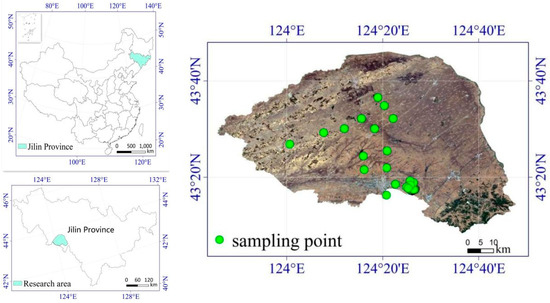
Figure 1.
Schematic of the study area and sampling site locations.
2.2. Data Sources for Remote Sensing
All Sentinel−2 remote sensing images used in the study were derived from the European Space Agency (ESA) Sentinel Scientific Data Hub (https://scihub.copernicus.eu/dhus/#/home) (accessed on 15 June 2022).
According to the study area’s topographic features and the images’ cloudiness, three sets of Sentinel−2 MSI images were selected at different times within a specific period. The images are from the UTM−WGS84 coordinate system, one set of four Sentinel−2 MSI images of different areas; the front and back sets are the baseline images, and the middle set of images is used to verify the accuracy of the prediction results. The downloaded Sentinel−2 MSI images are MSIL2A level data, which have been preprocessed and do not require pre−correction work. Thus, the images are directly cropped and stitched.
The MOD09GA image selected was obtained from NASA.com: https://urs.earthdata.nasa. The downloaded MOD09GA image was re−projected to UTM−WGS84 using the MODIS Reprojection Tool, cropped and stitched, and resampled to 20 m resolution using bilinear interpolation. The processed image is consistent with the above obtained Sentinel−2 image in terms of range shape, data resolution, cell size, and projection. The Sentinel−2 and MODIS band correspondence is shown in Table 1, and time correspondence and usage are shown in Table 2.

Table 1.
Sentinel−2 and MODIS bands used for the MRC estimation.
Table 2.
Sentinel−2 and MODIS acquisition time and usage.
2.3. Field Measurements
From 12–13 June 2021, the sampling points of maize MRC in the study area were photographed and sampled; then, the MRC of the sampling points was extracted using image processing [43]. The sampling points were selected in the vicinity of the farmland where there were no other features, such as poles and trees, to avoid the influence of other features on later image processing as much as possible. Furthermore, the sampling points were distributed as evenly as possible to comprehensively represent the different MRC situations in the study area. In total, 50 sampling points were selected, and ten images distributed in the shape of a cross were captured at each sampling point. The photos were taken with a phone that was kept flat on the ground, and the size of each photo was kept consistent. First, the photos at each sampling point were classified using the maximum−likelihood method in ENVI5.3. Then, the classification results were modified and adjusted according to visual inspection. Finally, the MRC was determined from the ratio of the number of pixels occupied by crop residue to the total number of pixels.
2.4. Methods
2.4.1. ESTARFM Algorithm
The ESTARFM algorithm was modified from STARFM by improving the conversion coefficient and the method for selecting similar image pixels in the heterogeneous range; thus, ESTARFM affords better predictions in heterogeneous regions than STARFM, and it has been widely used in the literature [44]. The ESTARFM algorithm developed by Zhu et al. [33] is based on the fusion of high spatial resolution images (Sentinel−2 images used herein) and high temporal resolution images (MODIS images used herein) from before and after a reference date (: and ) as well as one or more high temporal resolution images (MODIS images) from the predicted date () into a high spatial and temporal resolution image. The process is divided into four steps: (1) Select the Sentinel−2 and MODIS input. (2) Use the crossover values of Sentinel−2 reflectance at and to determine similar image pixels in the sliding window (w) and the ground cover category (c). (3) Determine the number of similar image pixels within each window and calculate the weighting function () based on the adjacent image pixels’ spatial and spectral similarity at and . (4) Perform linear regression of the MODIS data with Sentinel−2 data at to determine the spectral conversion coefficient () of the image pixels to predict the image.
where L and M represent the and coordinates of the Sentinel−2 images, and MODIS image pixels, band (b), /2, /2 represent the coordinates of the central image pixels. Additionally, N is the number of similar image pixels in the sliding window used to create the weights and coefficients for the ith prediction date.
2.4.2. IB and BI Integration Methodology
Currently, the NDTI using Sentinel−2 images can be calculated as follows: eliminating “based on the spectral band calculation can well estimate the CRC.”
NDTI using Sentinel−2 images can be calculated as follows:
Here, b11 and b12 are the 11th and 12th bands of the Sentinel−2 remote sensing data, respectively.
However, which fusion order should be chosen based on the ESTARFM algorithm to obtain high accuracy and high frequency NDTI is still inconclusive. Therefore, after determining the optimal parameters, the experimental results of the two fusion methods of BI and IB are compared. The two methods are fused in different orders: (1) The BI scheme first performs fusion to obtain the corresponding band data and then calculates the NDTI according to the calculation formula. (2) The IB scheme first calculates NDTI according to the formula and then fuses it to obtain the direct NDTI. The results of the IB and BI schemes are compared with the NDTI calculated from the original images, and the results accuracy is evaluated to compare the effectiveness of the two schemes. Currently, the research method of using remote sensing technology to obtain the tillage index and to then perform MRC estimation is being increasingly developed. Moreover, the estimation accuracy of NDTI is the highest among various tillage indices, and it is widely used for MRC estimation [45].
2.4.3. MRC Estimation Model
Xiang et al. [24] determined a corresponding regression relationship between the tillage index and MRC in the study area. Xiang et al. [24] performed a linear fit between the measured MRC and various tillage indexes and found that the highest R2 between these two, NDTI and MRC, was 0.729, and the RMSE was 0.0571, which can be better used for MRC estimation. Among them, y is CRC, and x is NDTI:
y = 0.31 + 1.66x + 19.55x2 − 61.97x3
Daughtry et al. [46] determined that, unlike the spectrum of the soil, the absorption properties around 2100 nm in the reflectance spectrum of dry crop residue are very pronounced due to the lignin and cellulose in the crop residue. Thus, spectral information around 2100 nm is essential for identifying crop residue. The NDTI calculation involves the 12th band (2185.7 nm) of Sentinel−2; thus, the obtained NDTI well correlates with the MRC. Daughtry et al. [47] found that the higher the water content of the crop residue, the lower the reflectance in all bands, with two absorption bands around 1450 and 1960 nm (wavelengths > 1300 nm); the highest and lowest spectra denote dry crop residue and water, respectively. Therefore, the extraction of spectral information at wavelengths > 1300 nm and around 1450 and 1960 nm is essential for identifying crop residues containing water. NDTI was calculated using the 11th band (1610.04 nm) and 12th band (2185.7 nm) of Sentinel−2 data. The highest correlation between NDTI and MRC was obtained with an R2 of 0.729. Therefore, NDTI and the linear regression model were chosen to estimate MRC herein.
2.4.4. MRC Value Extraction from Photos via the Maximum Likelihood Method
The maximum likelihood method is one of the most commonly used classification algorithms employed for the supervised classification of different photos. It calculates the weighted distance or similarity value D of the photos pixels X to be classified into a known category Mc and then passes the Bayesian formula as follows:
Then, the photos pixels are classified into the class with the highest probability of belonging. Advantageously, the maximum likelihood method as a parametric classifier considers the variance–covariance of class distribution. For normally distributed data, the maximum likelihood method affords better classification results than other parametric classifiers [48].
MRC was estimated by the NDTI from ESTARFM and the empirical model constructed by Xiang et al. (2022). The measured MRC values were used to validate the estimation accuracy of the MRC estimation model.
3. Results
3.1. ESTARFM
To validate the accuracy of the fusion results of ESTARFM, the predicted and actual NDTI for 12 June 2020 were compared. As shown in Figure 2, the distributions of the predicted and actual NDTI images are comparable. This signifies that ESTARFM can reasonably predict the information of NDTI. However, the predicted images were blurred despite the more complex detail information (e.g., the detail enlargement in Figure 2). This was due to the significant large difference in the spatial resolution between the short−wave IR bands of Sentinel 2 and MODIS. Thus, the fusion algorithm had difficulty capturing the richly textured and arbitrarily distributed features.

Figure 2.
Comparison of the actual and predicted NDTI in the study area: (A) actual NDTI distribution; (B) predicted NDTI distribution; (C) detail enlargement of the actual NDTI distribution; and (D) detail enlargement of the predicted NDTI distribution.
The scatter plot of the correlation between the predicted and actual NDTI of the same date for the test area predicted by the IB scheme (Figure 3) shows that most of the points are distributed on either side of the 1:1 trend line. Therefore, the R2 of the two images reached 0.73, and ESTARFM can well simulate the NDTI spectral index for that date. Moreover, the RMSE between the predicted NDTI image and the NDTI image calculated by Sentinel−2 is 0.000117, which is a minimal RMSE value. Since the difference between the predicted image and the actual image is minimal, the image prediction quality is good. Thus, ESTARFM is suitable for regions with high landscape heterogeneity and has good characterization ability for complex surface features.

Figure 3.
IB and BI comparison chart.
Some points are distributed far from the 1:1 trend line, primarily because the selected baseline image and the predicted image were obtained from late May to mid−June, during which the crops are already grown, which has some negative influence on the NDTI calculation. Nevertheless, the non−cultivated areas in the figure are essential factors that cause the results to contain NDTI outliers, and the outliers affect the overall prediction accuracy.
Figure 3 presents the scatter plots of the predicted and actual NDTI on 12 June 2020 that were derived from the BI and IB fusion schemes. Most of the IB scheme points are distributed on either side of the 1:1 trend line with an R2 of 0.73 and RMSE of 0.000117, which is very effective. On the other hand, the BI scheme has fewer points distributed on either side of the 1:1 trend line compared to the IB scheme, with an R2 of 0.68 and RMSE of 0.000305, which is lower than that of the IB scheme. Therefore, the prediction accuracy of the IB fusion scheme is higher than that of the BI fusion scheme.
3.2. MRC Estimation Model Accuracy Validation
To analyze the accuracy of the classification results of the images, the classification results were verified using a confusion matrix. The confusion matrix was analyzed by comparing the actual photos with the classification results. The results of the confusion matrix are shown in Table 3. The overall accuracy of image extraction was 93.6%, and the Kappa coefficient was 0.91; hence, the maximum likelihood method satisfactorily extracts the MRC.
Table 3.
Confusion matrix of the classification results via the maximum likelihood method.
The MRC on 17 May 2021 was estimated from the predicted NDTI, as shown in Figure 4. Since the coordinates of the sampling point obtained from the image and the actual sampling point deviate, a slight offset may be present in the position of the sampling point after the image coordinates are imported. To accurately obtain the field MRC, the MRC was extracted from the estimated average of a 3 × 3−pixel window centered on the sampling point [49]. Then, the fit analysis was performed with the MRC of the actual image extracted on 12 June 2021, and the scatter plot is shown in Figure 5 with an R2 of 0.78 and RMSE of 0.00676.

Figure 4.
MRC distribution in the study area.
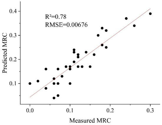
Figure 5.
Statistical relation between the field−sampled MRC and predicted MRC in the study area.
The predicted NDTI data selected for the estimation work inherently have some errors, which affect the accuracy of the estimation results. The selected MRC estimation model was compiled in February–March, which is a period when farmlands comprise more crop residues, the soil water content is lower than usual, and no crops have grown. Therefore, the model is less influenced by soil, water content, and crops and is suitable for MRC estimation in autumn and winter. However, the fieldwork of this study was conducted in May–June, when cultivated lands have less crop residue, high soil moisture content, and some growing crops. These factors affect the estimation accuracy of the model.
4. Discussion
4.1. Analysis of Fusion Methods
The NDTI data predicted by the IB scheme have R2 of 0.73 and RMSE of 0.000117, while the NDTI data predicted by the BI scheme have R2 of 0.68 and RMSE of 0.000305; the BI scheme affords lower R2 and RMSE than the IB scheme. Furthermore, using the IB scheme to predict the NDVI data, Guan et al. obtained R2 of 0.9534 and RMSE of 0.06553 and obtained R2 of 0.8657 and RMSE of 0.1032 using the BI scheme [38,50], showing that the BI scheme affords lower R2 and RMSE than the IB scheme. The above results denote that the IB scheme is better than the BI scheme in terms of R2 and RMSE, indicating that the IB scheme is better for the accuracy of the fusion results and image quality. This may be because the ESTARFM algorithm minimizes the systematic bias by exploiting the correlation between multi−source remote sensing data [33]. Furthermore, suppose that the temporal trend of the image pixel reflectance is linear, then, the relation between the high and low spatial resolution image pixel values can be deduced. Thus, high spatial resolution images are simulated for a specific date [30].
NDTI is an index established by scholars worldwide to characterize the MRC status based on the spectral reflectance characteristics of the crop residue and the waveband distribution characteristics of multi−spectral remote sensing data [23]. The effect of water vapor absorption in the atmosphere can be reduced by selecting appropriate remote sensing spectral bands in the atmospheric window. Additionally, standard deviation is a normalization algorithm that reduces the effect of the observation angle and atmospheric aerosols’ absorption and scattering effects. Nevertheless, these methods do not entirely eliminate the atmospheric effects [51]. Moreover, the NDTI constructed by combining the 11th and 12th bands of Sentinel−2 can significantly eliminate the interference of atmospheric aerosols on the tillage index, significantly improving the accuracy of MRC monitoring [52].
The IB scheme first calculates the index and then fuses it. Consequently, most errors are eliminated during the index calculation. Therefore, the number of errors generated during fusion is small, and the fusion results are better than those of the BI scheme. On the other hand, the BI scheme first fuses the images and then calculates the index; consequently, the image errors are amplified during the fusion process, leading to even more significant errors in the final results. Furthermore, the IB scheme only needs to predict the remote sensing index calculated from one band combination, while the BI scheme needs to predict two images from two bands and thus takes twice as long as the IB scheme. Hence, the IB scheme is more efficient and more accurate than the BI scheme. Subsequently, the IB scheme is more suitable than the BI scheme for ESTARFM to predict the crop residue remote sensing index with high frequency and high accuracy.
4.2. MRC Spatial Distribution Analysis
While the primary basis for tillage practices discrimination is MRC, Xiang et al. [24] classified MRC based on the CTIC criteria: MRC > 30% is conservation tillage and MRC < 30% is CT [10]. Herein, the tillage practices in the study area were classified according to the latest criteria: 0–15% MRC is CT, 15–30% is RT, and >30% MRC is NT [11]. Using the identification criteria for tillage patterns can provide a more detailed description of the spatial distribution of the various tillage patterns in the study area and is a sound basis for conservation tillage promotion and monitoring by the agricultural department.
ESTARFM predicted an image of 17 May 2021, a period when corn plowing in the study area was completed. The spatial distribution of the conservation tillage is shown in Figure 6. The NT and RT areas account for about 13% and 19% of the total cultivated land area, respectively. This result is more in line with previous reports on agricultural land management, wherein Zheng et al. based on a survey concluded that about 12% of the maize arable land is NT [53].

Figure 6.
Spatial distribution of conservation tillage in the study area.
As shown in Figure 6, RT and NT in Lishu County are primarily distributed in the southern part of Lishu County, which may be due to the implementation of the national conservation tillage policy. Since July 2020, the Jilin provincial government has promulgated and implemented the first local regulation in the country, the Jilin Province Black land Protection Regulation, to promote the gathering of talents, funds, and projects toward black land protection [54]. The southern part is mostly a demonstration site built by the government for conservation tillage technology [55].
Regarding the spatial distribution of the conservation tillage, the plots with conservation tillage measures are mainly concentrated in the southwestern part of Lishu County, which is close to residential areas and has a relatively flat topography [56]. This is because the number of NT planters was still relatively lacking in the early stages of conservation tillage promotion. Only a limited tillage area could be covered throughout the sowing period; thus, the areas close to urban areas and with flat terrains naturally became the preferred choice [57]. Moreover, it is currently tricky for NT planter machineries to work on steeply sloping arable land, which limits the rate of conservation tillage advancement in undulating terrains. The average annual precipitation in Lishu County is 558.4 mm, the precipitation decreases from the southeast to northwest, and minimum precipitation mainly occurs in the northwest. The average annual precipitation in the northwest is 462 mm [58]. Therefore, the northwestern arable land is mainly tilled with RT or NT to ensure crop growth from drought stress.
The eastern region is low−lying, with aeolian and saline soils in the farmland, and is dominated by wind−deposited alluvial terrain, accounting for 34% of the total area. Consequently, the soil organic matter in this region is relatively lower than that in other parts of Lishu County, with values ranging from 0.91 to 13.11 g/kg. Furthermore, the soil fertility and moisture retention are poor. Therefore, the region primarily uses RT and NT techniques to reduce the impact of maize yield due to drought.
4.3. Limitations and Prospects
This study constructs ESTARFM to predict the high spatial and temporal resolution NDTI and estimate the MRC. The model better predicts spectral data with fine plots and landscape heterogeneity than STARFM [31]. However, ESTARFM can be affected by the quality of MODIS and Sentinel−2 images of the baseline and the MODIS images of the predicted date. To avoid cloud influence on the NDTI prediction results as much as possible, the remote sensing images selected herein all contain less than 10% cloud cover. The MRC of the field photos was extracted via supervised classification and used to validate the MRC estimation results. However, the method can still be improved.
Guan et al. used ESTARFM to predict NDVI to investigate the model’s applicability in the middle and lower reaches of the Yangtze River plain. They showed that the prediction accuracy of NDVI can reach 95% [50]. Chen et al. employed ESTARFM to predict NDVI to extract irrigated cropland in the Chagannur watershed and obtained an R2 of 0.94 between their predicted and actual NDVI [29]. The predictions of NDVI based on ESTARFM in the above two studies yielded R2 of >0.9. In contrast, an R2 of only 0.73 was obtained herein. Therefore, to further improve the prediction accuracy, future research needs to identify and address the factors affecting the prediction accuracy of NDTI.
Xiang et al. compared the correlation of various tillage indices with MRC. The highest R2 correlation of 0.729 was found to be between NDTI and MRC. The MRC estimation model was constructed using NDTI and in situ MRC data collected in the fall of 2019 [24]. However, the model’s applicability for MRC inversion in spring needs to be further improved. In future research, in situ MRC data in spring need to be collected, and a corresponding spring MRC estimation model needs to be constructed to improve the model’s accuracy. Based on this model, the spring MRC can be predicted and the regional tillage practices can be classified.
5. Conclusions
In this study, the high spatial resolution Sentinel−2 images, high temporal resolution MODIS remote sensing images, and ESTARFM were utilized to predict the maize NDTI for a specific date. The accuracy of two prediction schemes, IB and BI, was compared using the actual NDTI data. The maize MRC in Lishu County was estimated using the MRC estimation model and the predicted NDTI. Furthermore, the study area’s tillage practices on maize farmland were identified according to the MRC tillage practices’ discriminatory criteria. Therefore, the following conclusions can be drawn:
This study predicted more available NDTI data based on ESTARFM than actual remote sensing images. Between the predicted and actual NDTI, the R2 was 0.73 and the RMSE was 0.000117, signifying that the ESTARFM accuracy meets the study requirements. The proposed method provided more available data sources for remote sensing monitoring of conservation tillage than previous methods.
Two forecasting schemes, IB and BI, were compared. The comparison revealed that the NDTI predicted by the IB scheme is not only better in model accuracy (R2 and RMSE), but also more efficient and less time consuming in the prediction process compared to the BI scheme. This finding is beneficial for studies requiring the prediction of remote sensing indices.
However, the prediction accuracy of ESTARFM is not as high as that of some previous methods, such as crop growth, as evidenced by the fact that the R2 of the predicted and actual NDTI did not exceed 0.8. This may stem from the fact that no further localization of the ESTARFM algorithm was performed. Moreover, a MRC estimation model applicable to spring was not employed. To address the above shortcomings, the original ESTARFM model needs to be improved to find the best model parameters that are more suitable for the study area, making the model more suitable for the prediction work. MRC sampling in the study area should be conducted to construct a more accurate spring MRC estimation model using the measured MRC data collected in the spring. Further exploration of remote sensing monitoring methods for conservation tillage on a larger scale and more extended time series is necessary.
Author Contributions
Conceptualization, J.D. and D.J.; methodology, J.D. and D.J.; software, D.J.; validation, D.J. and Y.Z. ; formal analysis, J.D. and D.J.; investigation, D.J., W.Z. and B.Z.; resources, Y.Z. and B.Z.; data curation, D.J.; writing—original draft preparation, D.J. and J.D.; writing—review and editing, J.D.; visualization, W.Z.; supervision, J.D.; project administration, J.D.; funding acquisition, J.D. and K.S. All authors have read and agreed to the published version of the manuscript.
Funding
This research was funded by the National Key Research and Development Program of China (No. 2021YFD1500103), the Science and Technology Project for Black Soil Granary (No. XDA28080500), and the National Science & Technology Fundamental Resources Investigation Program of China (No. 2018FY100300).
Data Availability Statement
Not applicable.
Acknowledgments
The authors would like to thank the anonymous reviewers for their valuable comments on the manuscript, which helped improve the quality of the paper. We would also like to thank Charlesworth Author Services for English language editing.
Conflicts of Interest
The authors declare no conflict of interest. The funders had no role in the design of the study; in the collection, analyses, or interpretation of data; in the writing of the manuscript; or in the decision to publish the results.
References
- Meng, F.; Yu, X.; Gao, J. The bottleneck and breakthrough path of the conservation tillage development in black soil of northeast China. J. Issues Agric. Econ. 2020, 2, 135–142. [Google Scholar]
- Li, A.; Fan, X.; Wu, C. Situation and development trends of conservation tillage in the world. Trans. Chin. Soc. Agric. Mach. 2006, 37, 177–180. [Google Scholar]
- Liu, W.; Li, W.; Zheng, K.; Zhao, H. The current research status of conservation tillage technology. J. Agric. Mech. Res. 2017, 39, 256–261+268. [Google Scholar]
- Vaneph, S.; Benites, J. First World Congress on Conservation Agriculture A World−Wide Challenge. R. Madrid, Spain, 1–5 October 2001. Available online: http://www.act-africa.org/file/newsletters/books_manuals/first-wcca%20.pdf (accessed on 21 November 2022).
- Kassam, A.; Friedrich, T.; Derpsch, R. Worldwide adoption of conservation agriculture. In Proceedings of the 6th World Congress on Conservation Agriculture, Winnipeg, MB, Canada, 21–25 June 2014; pp. 22–25. [Google Scholar]
- Derpsch, R. Historical review of no−tillage cultivation of crops. In Proceedings of the Conservation Tillage for Sustainable Agriculture. Proceedings from an International Workshop, Harare, Zimbabwe, 22–27 June 1998; pp. 22–27. [Google Scholar]
- Derpsch, R.; Friedrich, T. Global overview of conservation agriculture adoption. In Proceedings of the World Congress on Conservation Agriculture, New Delhi, India, 4–7 February 2009. [Google Scholar]
- Kassam, A.; Friedrich, T.; Derpsch, R. Overview of the worldwide spread of conservation agriculture. Field Actions Sci. Rep. J. Field Actions 2015, 8, 12–15. [Google Scholar]
- Ao, M.; Zhang, X.; Guan, Y. Research and practice of conservation tillage in black soil region of northeast China. Bull. Chin. Acad. Sci. 2021, 36, 1203–1215. [Google Scholar]
- CTIC. Tillage Type Definitions; Conservation Technology Information Center: West Lafayette, IN, USA, 2016. [Google Scholar]
- Najafi, P.; Navid, H.; Feizizadeh, B. Object−based satellite image analysis applied for crop residue estimating using Landsat OLI imagery. Int. J. Remote Sens. 2018, 39, 6117–6136. [Google Scholar] [CrossRef]
- Carter, M. Conservation Tillage. In Encyclopedia of Soils in the Environment; Academic Press: Cambridge, MA, USA, 2005; pp. 306–311. [Google Scholar]
- Morrison, J. Strip tillage for “no–till” row crop production. Appl. Eng. Agric. 2002, 18, 277. [Google Scholar] [CrossRef]
- Zhou, J.; Khot, L.; Boydston, R.; Miklas, P.N.; Porter, L. Low altitude remote sensing technologies for crop stress monitoring: A case study on spatial and temporal monitoring of irrigated pinto bean. Precis. Agric. 2018, 19, 555–569. [Google Scholar] [CrossRef]
- Sullivan, D.; Lee, D.; Beasley, J.; Brown, S.; Williams, E.J. Evaluating a crop residue cover index for determining tillage regime in a cotton−corn−peanut rotation. J. Soil Water Conserv. 2008, 63, 28–36. [Google Scholar] [CrossRef]
- Zheng, D.; Jiang, H.; Li, B.; Li, H.; Zhang, J. Study on the no−tillage mulch planter for wheat under the bestrow of the whole mealie straw. J. Agric. Univ. Hebei 2003, S1, 285–287. [Google Scholar]
- Gong, J.; Huang, G.; Chen, L.; Fu, B. Comprehensive ecological effect of straw mulch on spring wheat field in dry land area. Agric. Res. Arid. Areas 2003, 03, 69–73. [Google Scholar]
- Yang, S.; Yang, K. Cybernetics Foundation for Mechanical Engineering; Huazhong University of Science and Technology Publishing: Wuhan, China, 2002; pp. 154–196. [Google Scholar]
- Zhang, Z. Proficient in Matlab 6.5.; Beihang University Press: Beijing, China, 2003; pp. 126–143. [Google Scholar]
- Yu, G.; Hao, R.; Ma, H.; Wu, S.; Chen, M. Research on Image Recognition Method Based on SVM Algorithm and ESN Algorithm for Crushed Straw Mulching Rate. J. Henan Agric. Sci. 2018, 47, 155–160. [Google Scholar]
- McCarty, J.; Loboda, T.; Trigg, S. A hybrid remote sensing approach to quantifying crop residue burning in the United States. Appl. Eng. Agric. 2008, 24, 515–527. [Google Scholar] [CrossRef]
- Van Deventer, A.P.; Ward, A.D.; Gowda, P.H. Using thematic mapper data to identify contrasting soil plains and tillage practices. Photogramm. Eng. Remote Sens. 1997, 63, 87–93. [Google Scholar]
- Jin, X.; Ma, J.; Wen, Z.; Song, K. Estimation of maize residue cover using Landsat−8 OLI image spectral information and textural features. Remote Sens. 2015, 7, 14559–14575. [Google Scholar] [CrossRef]
- Xiang, X.; Du, J.; Jacinthe, P.A. Integration of tillage indices and textural features of Sentinel−2A multispectral images for maize residue cover estimation. Soil Tillage Res. 2022, 221, 105405. [Google Scholar] [CrossRef]
- Cai, W.; Zhao, S.; Wang, Y. Estimation of winter wheat residue cover using spectral and textural information from Sentinel−2 data. Remote Sens. 2020, 24, 1108–1119. [Google Scholar]
- Bannari, A.; Pacheco, A.; Staenz, K. Estimating and mapping crop residues cover on agricultural lands using hyperspectral and IKONOS data. Remote Sens. Environ. 2006, 104, 447–459. [Google Scholar] [CrossRef]
- Ding, Y.; Zhang, H.; Wang, Z. A comparison of estimating crop residue cover from sentinel−2 data using empirical regressions and machine learning methods. Remote Sens. 2020, 12, 1470. [Google Scholar] [CrossRef]
- Zheng, B.; Campbell, J.B.; Shao, Y. Broad−scale monitoring of tillage practices using sequential landsat imagery. Soil Sci. Soc. Am. J. 2013, 77, 1755–1764. [Google Scholar] [CrossRef]
- Chen, X.; Wang, Y.; Zhang, H.; Liu, F. Extraction method of irrigated arable land in the Chahannur Basin based on the ESTARFM NDVI. Chin. J. Ecoagric. 2021, 29, 1105–1116. [Google Scholar]
- Huang, B.; Zhang, H.; Song, H. Unified fusion of remote−sensing imagery: Generating simultaneously high−resolution synthetic spatial–temporal–spectral earth observations. Remote Sens. 2013, 4, 561–569. [Google Scholar] [CrossRef]
- Gao, F.; Masek, J.; Schwaller, M. On the blending of the Landsat and MODIS surface reflectance: Predicting daily Landsat surface reflectance. IEEE Trans. Geosci. Remote Sens. 2006, 44, 2207–2218. [Google Scholar]
- Knauer, K.; Gessner, U.; Fensholt, R. An ESTARFM fusion framework for the generation of large−scale time series in cloud−prone and heterogeneous landscapes. Remote Sens. 2016, 8, 425. [Google Scholar] [CrossRef]
- Zhu, X.; Chen, J.; Gao, F. An enhanced spatial and temporal adaptive reflectance fusion model for complex heterogeneous regions. J. Remote Sens. Environ. 2010, 114, 2610–2623. [Google Scholar] [CrossRef]
- Emelyanova, I.; McVicar, T.; Van Niel, A.I. Assessing the accuracy of blending Landsat–MODIS surface reflectances in two landscapes with contrasting spatial and temporal dynamics: A framework for algorithm selection. J. Remote Sens. Environ. 2013, 133, 193–209. [Google Scholar] [CrossRef]
- Chen, B.; Huang, B.; Xu, B. Comparison of spatiotemporal fusion models: A review. Remote Sens. 2015, 7, 1798–1835. [Google Scholar] [CrossRef]
- Liao, C.; Wang, J.; Pritchard, I. A spatio−temporal data fusion model for generating NDVI time series in heterogeneous regions. Remote Sens. 2017, 9, 1125. [Google Scholar] [CrossRef]
- Watts, J.; Powell, S.; Lawrence, R. Improved classification of conservation tillage adoption using high temporal and synthetic satellite imagery. J. Remote Sens. Environ. 2011, 115, 66–75. [Google Scholar] [CrossRef]
- Jarihani, A.; McVicar, T.; Van, N. Blending Landsat and MODIS data to generate multispectral indices: A comparison of “Index−then−Blend” and “Blend−then−Index” approaches. Remote Sens. 2014, 6, 9213–9238. [Google Scholar] [CrossRef]
- Guo, X.; Kang, Y. Research on arable land protection from the perspective of new agricultural operators. Agric. Technol. 2021, 41, 152–155. [Google Scholar]
- Li, Z.; Cao, W.; Liu, B.; Luo, Z. Current status and developing trend of soil erosion in China. Sci. Soil Water Conserv. 2008, 01, 57–62. [Google Scholar]
- Yang, X.; Guo, J.; Liu, H.; Liu, B. Soil wind erosion environment in black soil region in Northeastern China. Sci. Geogr. Sin. 2006, 4, 4443–4448. [Google Scholar]
- Wang, C.; Tu, Z.; Zheng, T. Study on promotion and application of conservation tillage technology in Jilin. Chin. Agric. Mech. 2019, 40, 200–203. [Google Scholar]
- Li, H.; Li, H.; He, J. Measuring system for residue cover rate in field based on bp neural network. Trans. Chin. Soc. Agric. Mach. 2009, 40, 58–62. [Google Scholar]
- Zhu, X.; Cai, F.; Tian, J. Spatiotemporal fusion of multisource remote sensing data: Literature survey, taxonomy, principles, applications, and future directions. Remote Sens. 2018, 10, 527. [Google Scholar] [CrossRef]
- Xiang, X.; Du, J.; Zhao, B.; Zhou, H.; Song, K. Remotely sensed estimation of maize residue cover in typical agricultural regions of Songnen Plain. Soil Crops 2021, 10, 282–293. [Google Scholar]
- Daughtry, C.S.T. Discriminating crop residues from soil by shortwave infrared reflectance. Agron. J. 2001, 93, 125–131. [Google Scholar] [CrossRef]
- Daughtry, C.; Hunt, E., Jr.; McMurtrey, J., III. Assessing crop residue cover using shortwave infrared reflectance. Remote Sens. Environ. 2004, 90, 126–134. [Google Scholar] [CrossRef]
- ERDAS (Firm). ERDAS Field Guide; ERDAS: Huntsville, AL, USA, 1997. [Google Scholar]
- Guo, Y. Calibration and validation of the microwave humidity and temperature detector of the Fengyun−3C satellite. Chin. J. Geotech. 2015, 58, 12. [Google Scholar]
- Guan, Q.; Ding, M.; Zhang, H. Analysis of applicability about ESTARFM in the middle−lower Yangtze Plain. J. Geoinform. Sci. 2021, 23, 1118–1130. [Google Scholar]
- Li, X.; Liu, S. Principles and Applications of Remote Sensing; Science Press: Beijing, China, 2008. [Google Scholar]
- Kaufman, Y.J.; Tanre, D. Atmospherically resistant vegetation index (ARVI) for EOS−MODIS. IEEE Trans. Geosci. Remote Sens. 1992, 30, 261–270. [Google Scholar] [CrossRef]
- Zheng, T.; Zhai, K.; Zou, S. A survey of corn conservation tillage in Jilin Province of China. Agric. Mach. Technol. Extend 2016, 4, 7–9. [Google Scholar]
- Yan, H. Create “Lishu model” upgraded version. Jilin Dly. 2022, 2, 3–5. [Google Scholar]
- Geng, D. Investigation and Analysis of the Promotion and Application of Straw Returning in Jilin Province; Jilin Agricultural University: Changchun, China, 2016. [Google Scholar]
- Liu, X. Study on the Problems and Countermeasures of Water Resources in Lishu County. J. Intell. 2011, 25, 304. [Google Scholar]
- Cui, N.; Fan, Y.; Dong, J. Application status and developing routes of maize straw mulching of conservation tillage technology in Northeast China. J. Mai Sci. 2021, 29, 112–117+126. [Google Scholar]
- Sheng, W.; Bai, Y. Analysis of water resources status in Lishu County. Bus. China 2010, 7, 395. [Google Scholar]


Disclaimer/Publisher’s Note: The statements, opinions and data contained in all publications are solely those of the individual author(s) and contributor(s) and not of MDPI and/or the editor(s). MDPI and/or the editor(s) disclaim responsibility for any injury to people or property resulting from any ideas, methods, instructions or products referred to in the content. |
© 2023 by the authors. Licensee MDPI, Basel, Switzerland. This article is an open access article distributed under the terms and conditions of the Creative Commons Attribution (CC BY) license (https://creativecommons.org/licenses/by/4.0/).