A Geometric Multigrid Method for 3D Magnetotelluric Forward Modeling Using Finite-Element Method

Abstract

The traditional three-dimensional (3D) magnetotelluric (MT) forward modeling using Krylov subspace algorithms has the problem of low modeling efficiency. To improve the computational efficiency of 3D MT forward modeling, we present a novel geometric multigrid algorithm for the finite element method. We use the vector finite element to discretize Maxwell’s equations in the frequency domain and apply the Dirichlet boundary conditions to obtain large sparse complex linear equations for the solution of EM responses. To improve the convergence of the solution at low frequencies we use the divergence correction to correct the electric field. Then, we develop a V-cycle geometric multigrid algorithm to solve the linear equations system. To demonstrate the efficiency and effectiveness of our geometric multigrid method, we take three synthetic models (COMMEMI 3D-2 model, Dublin test model 1, modified SEG/EAEG salt dome model) and compare our results with the published ones. Numerical results show that the geometric multigrid algorithm proposed in this paper is much better than the commonly used Krylov subspace algorithms (such as SOR-GMRES, ILU-BICGSTAB, SOR-BICGSTAB) in terms of the iteration number, the solution time, and the stability, and thus is more suitable for large-scale 3D MT forward modeling.

1. Introduction

Magnetotelluric (MT) is a geophysical exploration method that uses the natural electromagnetic (EM) field as the source and obtains the underground electrical structure by observing the mutually orthogonal EM field components at the earth surface [1,2]. This method has been widely used in mineral and hydrocarbon exploration [3,4,5], geothermal detection [6], groundwater exploration [7], prediction of earthquake precursors [8], and studies of deep electrical structures [9].

Fast and accurate three-dimensional (3D) MT forward modeling is the key to the inversion and interpretation of MT data. The numerical methods commonly used in the EM simulation mainly include the integral equation method (IE) [10,11], the finite difference method (FD) [12,13,14], the finite volume method (FV) [15,16] and the finite element method (FE) [17,18]. Currently there are several tools available [14,19,20]. The FE method has the advantages of high accuracy, flexibility and applicability for complex underground structures. In particular, the vector FE method has now become the mainstream method of numerical EM simulation, for it can effectively solve the problem of pseudo-solutions in node FE method [21,22,23,24,25,26,27].

The most time-consuming part in MT forward modeling is the solution of linear equations system. This means that the key to improving the efficiency of forward modeling is to shorten the time for the solution of the linear equations system. The methods for solving the linear equations include the direct methods and the iterative ones. The direct methods obtain the solution of the equations system through finite algebraic operations. The common direct solvers include MUMPS, PARDISO, SuperLU, etc. Scholars have used different direct methods in the solution of the linear equations system in 3D MT forward modeling [17,24,28,29]. The advantage of direct methods is their robustness, but they require a lot of computer memory and thus are only suitable for small to medium-sized problems. The iterative methods start from a given initial value and iteratively approach the exact solution that requires far less computer memory than the direct methods. The commonly used iterative algorithms are generally based on Krylov subspaces, such as the biconjugate gradient stabilized method (BiCGSTAB) [30], the quasi-minimal residual method (QMR) [31], the generalized minimal residual method (GMRES) [32], etc. Since the condition number of the linear equations system obtained by discretizing the Maxwell equation system is generally very large, it is necessary to use preconditioning techniques to reduce the condition number of the coefficient matrix, such as the Jacobi preconditioning (Jacobi) [33], the successive over relaxation preconditioning (SOR) [34], the incomplete LU factorization preconditioning (ILU) [31]. As the frequency decreases, the convergence of the iterative methods will deteriorate, and a divergence correction technique is generally required to improve the convergence of the iterative algorithm [35,36,37]. Due to the large number of null spaces in the curl-curl operator involved in solving the equation for the electric field, even with preconditioning and divergence corrections, the convergence is still very slow. With an increasing model scale, the number of iterations and solution time will increase sharply, the traditional iterative algorithms have difficulty in handling large-scale 3D MT modeling problems.

The multigrid algorithm (MG) is one of the most effective iterative methods for solving large-scale linear equations. It has the advantages of fast convergence, and its convergence is independent of the grids [38]. This method includes geometric multigrid (GMG) [39,40,41,42,43,44] and algebraic multigrid (AMG) [45,46,47,48]. The geometric multigrid uses geometric information from nested grids to construct operational operators. It is straightforward to implement. It requires less memory and has advantages over algebraic multigrid in problems using structured grids. The algebraic multigrid uses the system matrix information to construct operators. It has strong versatility and is suitable for structured and unstructured problems. However, it needs an expensive setup, both in time and memory [49]. Mulder (2006, 2008) used the geometric multigrid method as an independent solver and a preprocessing operator for BICGSTAB to solve the EM equations discretized by the finite volume (FV) method; it has good convergence under uniform grids, but the convergence rate decreases under the stretched grid [39,40]. Koldan et al. (2014) used the algebraic multigrid method as the preprocessing operator for the Krylov subspace method and effectively reduced the time for 3D EM simulation based on the nodal FE method [45]. Jaysaval et al. (2016) used the geometric multigrid as the preconditioner for BICGSTAB to solve the large linear equations system generated by discretizing the frequency-domain Maxwell’s equations for the FD method on the Lebedev grid [41]. Li et al. (2016) used the geometric multigrid method combined with the magnetic field divergence correction to solve 3D EM modeling problems using FD on Yee’s grids [42]. Yao et al. (2021) used the FGMRES method with algebraic multigrid preconditioning to solve the global EM induction using the FE method based on the magnetic vector potential and electric scalar potential [48]. Guo et al. (2022) proposed a geometric multigrid algorithm based on a four-color Gauss-Seidel smoothing algorithm for 3D MT forward simulation by the FD method [43]. Pan et al. (2022) developed an improved extrapolation cascade multigrid method (iEXCMG) to solve the large linear equations system generated by FE discretization of Maxwell’s equations based on EM potentials on non-uniform orthogonal grids [44].

At present, the research on the multigrid method in EM forward modeling mainly focuses on using it as a preconditioning technique to accelerate the solution of the Krylov subspace iterative method. This does not take full advantage of the multigrid method. Moreover, most current studies combine the multigrid method with numerical simulations using the FD and FV methods. Although there are reports on multigrid methods used in node FE for solving the electric field, the magnetic vector, and the electric scalar potentials, there are few reports on the multigrid algorithm for the solution of the curl-curl equations of the electric field using the vector FE method. Since the vector FE method can effectively avoid the pseudo-solutions of the nodal FE method and the curl-curl equation for the electric field has fewer unknowns than the vector-scalar potential equation, we develop in this paper an efficient 3D MT forward modeling method by combining the geometric multigrid method with the vector FE method for solving the curl-curl equation of the electric field.

In the sequence, we first introduce the methodology for 3D MT forward modeling, including the governing equation, the vector FE discretization and the calculation of impedance apparent resistivities and phases, then we use divergence correction to improve the convergence of the iterative solution. After that, we develop the geometric multigrid algorithm to solve the linear equations system. Finally, we verify the accuracy of the algorithm with a three-layer model and test the numerical performance of the algorithm with three typical synthetic models.

2. Methods

2.1. 3D MT Forward Modeling

Assuming a time dependence of e^iωt and ignoring the displacement current, we get Maxwell’s equations in the frequency-domain, i.e.,

$$\nabla \times \mathit{E}=-i\omega {\mu }_0\mathit{H},$$

(1)

$$\nabla \times \mathit{H}=\sigma \mathit{E}+{\mathit{J}}_p,$$

(2)

where ω is the angular frequency, E is the electric field, and H is the magnetic field, μ₀ = 4π × 10⁻⁷ H/m is the vacuum magnetic permeability, σ is the conductivity, J_p is the source current density.

We divide the total field into the primary and secondary parts, E = E_p+ E_s, H = H_p + H_s, then substitution into Equations (1) and (2) yields

$$\nabla \times {\mathit{E}}_s=-i\omega {\mu }_0{\mathit{H}}_s,$$

(3)

$$\nabla \times {\mathit{H}}_s=\sigma {\mathit{E}}_s+{\mathit{J}}_p,$$

(4)

where ${\mathit{J}}_p=\left(\sigma -{\sigma }_0\right){\mathit{E}}_p={\sigma }_a{\mathit{E}}_p$ is the new source term, ${\sigma }_0$ is the background conductivity, ${\sigma }_a=\sigma -{\sigma }_0$ is the abnormal conductivity.

Taking the curl on both sides of (3) and substituting (4) into it, we obtain the curl-curl equation for the secondary electric field in the frequency-domain, i.e.,

$$\nabla \times \nabla \times {\mathit{E}}_s+i\omega {\mu }_0\sigma {\mathit{E}}_s=-i\omega {\mu }_0{\sigma }_a{\mathit{E}}_p.$$

(5)

To ensure the unique solution of Equation (5), we adopt the Dirichlet boundary conditions:

$${\mathit{E}}_s\left|{}_{\mathsf{\Gamma }}\right.=0.$$

(6)

To solve the EM field from Equations (5) and (6), we discretize the computational domain into multiple hexahedral elements and put the electric field components on the edges [50], so that the electric field within each element can be written as

$${\mathit{E}}^e={\displaystyle \sum _{i=1}^{12}{{\displaystyle \mathit{N}}}_i^e}{{\displaystyle E}}_i^e,$$

(7)

where ${{\displaystyle \mathit{N}}}_i^e$ represents the vector interpolation basis function at the i-th edge in the element [21], ${{\displaystyle E}}_i^e$ represents the tangential electric field at the same edge.

Taking the dot product of Equation (5) with a vector basis function and applying the first vector Green’s Theorem, we obtain the weak form of Equation (5), namely.

$${\displaystyle {\int }_V\left(\nabla \times \mathit{N}\cdot \nabla \times {\mathit{E}}_s+i\omega {\mu }_0\sigma \mathit{N}\cdot {\mathit{E}}_s\right)dv}={\displaystyle {\int }_V\left(-i\omega {\mu }_0{\sigma }_a\mathit{N}\cdot {\mathit{E}}_p\right)dv},$$

(8)

where V denotes the computational domain. Substituting Equation (7) into (8) and integrating, we get the linear equations system for each element, i.e.,

$${\displaystyle \sum _{i=1}^{12}{E}_{si}}{\displaystyle {\int }_V\left(\nabla \times \mathit{N}\right)\cdot \left(\nabla \times \mathit{N}\right)+i\omega {\mu }_0\sigma \mathit{N}\cdot \mathit{N}dv}={\displaystyle \sum _{i=1}^{12}{E}_{Pi}}{\displaystyle {\int }_V\left(-i\omega {\mu }_0{\sigma }_a\mathit{N}\cdot \mathit{N}\right)dv}.$$

(9)

Equation (9) can be rewritten in a matrix format, i.e.,

$${\mathbf{A}}^e{\mathit{e}}^e={\mathit{b}}^e,$$

(10)

where A^e denotes the coefficient matrix corresponding to element e, b^e is the source vector, e^e is the secondary electric field at the edge of the element. From Equations (9) and (10), we obtain

$${\mathbf{A}}^e={\displaystyle {\int }_V\left(\nabla \times \mathit{N}\right)\cdot \left(\nabla \times \mathit{N}\right)+i\omega {\mu }_0\sigma \mathit{N}\cdot \mathit{N}dv},$$

(11)

$${\mathit{b}}^e={\displaystyle \sum _{i=1}^{12}{E}_{Pi}}{\displaystyle {\int }_V\left(-i\omega {\mu }_0{\sigma }_a\mathit{N}\cdot \mathit{N}\right)dv}.$$

(12)

Assembling the matrix equations of all elements, we get the final linear equations system for the secondary electric field, i.e.,

$$\mathbf{A}\mathit{e}=\mathit{b},$$

(13)

where A is the coefficient matrix, b is the source term, and e denotes the unknown secondary electric fields. Solving Equations (13), we obtain the secondary electric field at each edge. The secondary electric fields at receiving points are calculated by interpolation using Equation (7). By adding the secondary and the primary field, we get the total field. Then, the magnetic field can be calculated by using Faraday’s law, i.e.,

$$\mathit{H}=\frac{1}{i\omega \mu }\nabla \times \mathit{E}.$$

(14)

After obtaining the EM fields $E_x^1$,$E_y^1$,$H_x^1$,$H_y^1$ for x-polarization mode and $E_x^2$, $E_y^2$, $H_x^2$, $H_y^2$ for y-polarization mode, we can calculate the MT impedance tensor by

$$\mathit{Z}=\left[\begin{array}{cc}{Z}_{xx}& Z_{xy}\\ Z_{yx}& Z_{yy}\end{array}\right],$$

(15)

where the components can be written as

$$\begin{gathered} Z_{xx}=\frac{E_x^1{H}_y^2-H_y^1{E}_x^2}{H_x^1{H}_y^2-H_y^1{H}_x^2},Z_{xy}=\frac{E_x^2{H}_x^1-H_x^2{E}_x^1}{H_x^1{H}_y^2-H_y^1{H}_x^2}, \\ {Z}_{yx}=\frac{E_y^1{H}_y^2-H_y^1{E}_y^2}{H_x^1{H}_y^2-H_y^1{H}_x^2},Z_{yy}=\frac{E_y^2{H}_x^1-H_x^2{E}_y^1}{H_x^1{H}_y^2-H_y^1{H}_x^2}. \end{gathered}$$

(16)

Finally, we can calculate the apparent resistivities and phases by

$${\rho }_{ij}=\frac{{\left|Z_{ij}\right|}^2}{\omega {\mu }_0},{\phi }_{ij}=arg\left(Z_{ij}\right),i,j=x,y.$$

(17)

2.2. Divergence Correction

When solving the curl-curl equation for the electric field by the iterative method, the solution process converges slowly as the frequency decreases. This is because the item $i\omega \mu \sigma \mathit{E}$ in the curl-curl equation becomes less important. This results in the divergence-free condition for the current density specified by Maxwell’s equations not being satisfied in the iterative process [51]. Therefore, we need to enforce the divergence-free condition by solving the following Poisson’s equation for the static potential φ [35,36,37], i.e.,

$$\nabla \cdot \left(\sigma \nabla \phi \right)=-\nabla \cdot \mathit{J}.$$

(18)

Note that in the solution of Equation (5), we use the vector FE method and assume the divergence-free vector basis function. Since the conductivity is constant within each cell, there is no accumulated charges inside the cell when the current passes through. Thus, in each cell Equation (18) can be simplified to

$$\nabla \cdot \left(\sigma \nabla \phi \right)=0.$$

(19)

On the interface of adjacent cells with different conductivities, there exists

$$\widehat{\mathbf{n}}\cdot \left({\sigma }_i\nabla {\phi }_i-{\sigma }_j\nabla {\phi }_j\right)\left|s_{ij}\right.=\widehat{\mathbf{n}}\cdot \left({\sigma }_i{\mathit{E}}_{si}-{\sigma }_j{\mathit{E}}_{sj}+{\sigma }_{ai}{\mathit{E}}_{pi}-{\sigma }_{aj}{\mathit{E}}_{pj}\right),$$

(20)

where i,j denote two adjacent cells. We adopt the Dirichlet boundary conditions and set the potential φ on the boundary to zero $\phi \left|{}_{\mathsf{\Gamma }}\right.=0$.

To use the nodal FE method to solve Equation (19), we write the potential φ as

$$\phi ={\displaystyle \sum _{n=1}^{N_{node}}{\phi }_n{u}_n},$$

(21)

where ${\phi }_n$ is the potential at the node, $u_n$ is the node basis function, N_node is the number of nodes in each element.

Using the Galerkin method to solve for the potential, we substitute Equation (21) into (19), multiply both sides by the node basis function $u_k$, and integrate within the cell and obtain

$${\displaystyle \sum _{n=1}^{N_{node}}{\displaystyle {\int }_V{u}_m}}\nabla \cdot \left(\sigma \nabla u_n\right)dv{\phi }_n=0.$$

(22)

Applying the first scalar Green’s theorem, for the i-th cell, we have

$${\displaystyle {\int }_{Vi}{u}_m\nabla \cdot \left({\sigma }_i\nabla u_n\right)dv}=-{\displaystyle {\int }_{Vi}{\sigma }_i\nabla u_m\cdot \nabla u_{n}dv}+{\displaystyle {\int }_{Si}{\sigma }_i{u}_m\nabla u_n}\cdot \widehat{\mathbf{n}}ds,$$

(23)

where ${\sigma }_i$ is the conductivity of the i-th cell. Using the interior boundary condition (20), the surface integral in the above equation can be written as

$${\displaystyle {\int }_{Si}{\sigma }_i{u}_m\nabla u_n\cdot \widehat{\mathbf{n}}}ds{\phi }_n={\displaystyle {\int }_{Si}{u}_m}\left({\sigma }_i{E}_{si}{\mathit{N}}_i+{\sigma }_{ai}{E}_{pi}{\mathit{N}}_i\right)\cdot \widehat{\mathbf{n}}ds,$$

(24)

where ${\mathit{N}}_i$ denotes the vector interpolation basis functions. Combining Equations (22)–(24), we obtain

$${\displaystyle \sum _{n=1}^{N_{node}}{\phi }_n{\displaystyle {\int }_V\sigma \nabla u_m\cdot \nabla u_{n}dv}}={\displaystyle \sum _{j=1}^N\left(E_{sj}{\displaystyle {\int }_S\sigma u_m{\mathit{N}}_j\cdot }\widehat{\mathbf{n}}ds+E_{pj}{\displaystyle {\int }_S{\sigma }_a{u}_m{\mathit{N}}_j\cdot \widehat{\mathbf{n}}ds}\right)},$$

(25)

where N denotes the number of edges in the current cell. Equation (25) can be written in a matrix format, i.e.,

$$\mathbf{D}\mathit{p}=\mathit{t},$$

(26)

where $D_{mn}={\displaystyle {\int }_V\sigma \nabla u_m\cdot \nabla u_{n}dv}$,$p_n={\phi }_n$,$t_m={\displaystyle \sum _{j=1}^N\left(E_{sj}{\displaystyle {\int }_S\sigma u_m{\mathit{N}}_j}\cdot \widehat{\mathbf{n}}ds+E_{pj}{\displaystyle {\int }_S{\sigma }_a{u}_m{\mathit{N}}_j\cdot \widehat{\mathbf{n}}ds}\right)}$ and m, n = 1, …, N_node.

After obtaining the scalar potential $\phi$, the electric field can be corrected by the following equation

$${\mathit{e}}_{new}={\mathit{e}}_{old}-\nabla \phi .$$

(27)

Using the divergence correction in Equation (27), the divergence-free condition is enforced. When solving Equation (13), we can apply the divergence correction every few iterations to speed up the iterative solution process.

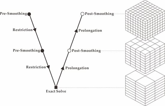
2.3. Multigrid Algorithm

The multigrid algorithm is not a single method; it is essentially an iterative scheme. Firstly, the high-frequency errors are eliminated by smoothing iterations on the fine grid. Then, the remaining low-frequency errors are transferred to a coarser grid, where the errors will become high-frequency again and can be effectively eliminated by several smoothing iterations. By repeating this process until the pre-designed coarsest grid, the scale of the problems to be solved will become very small, so that we can achieve the solution quickly by a direct solver. Finally, the solution is interpolated step by step from the coarsest grid to the fine one to correct the solution for the fine grid. This is the so-called coarse grid correction strategy that is the core of the multigrid algorithm.

There are many cycle structures for the multigrid algorithm to convert between coarse and fine grids. The commonly used cycle structure includes V-cycle, W-cycle, and FMV cycle, as shown in Figure 1. The cycle structure is selected according to the complexity of the problem. Based on the large number of numerical tests, the performance differences between V-cycle, W-cycle, and FMV cycle are not very obvious. The V-cycle has the characteristics of simple implementation and small calculation amount, so we use it in our following model calculations.

We take the simplest two-level multigrid V-cycle as an example to illustrate the calculation process of the multigrid method (k and k-1 represent the step sizes of the fine grid and coarse grid, respectively).

• Pre-smoothing: n₁ times of smoothing iterations on the fine grid to obtain the approximate solution ${\tilde{\mathit{e}}}^k$ of Equation (13) ${\mathbf{A}}^k{\mathit{e}}^k={\mathit{b}}^k$. In this step, the high-frequency errors are eliminated, but the low-frequency errors remain.
• Compute residual: The residual vector ${\mathit{r}}^k$ corresponding to the approximate solution ${\tilde{\mathit{e}}}^k$ on the fine grid is calculated by ${\mathit{r}}^k={\mathit{b}}^k-{\mathbf{A}}^k{\tilde{\mathit{e}}}^k$.
• Restriction: Using the restriction matrix ${\mathbf{R}}_k^{k-1}$ to project the residual vector ${\mathit{r}}^k$ onto the coarse grid, i.e., ${\mathit{b}}^{k-1}={\mathbf{R}}_k^{k-1}{\mathit{r}}^k$.
• Solve the residual equation: Solving the residual equation ${\mathbf{A}}^{k-1}{\mathit{e}}^{k-1}={\mathit{b}}^{k-1}$ on a coarse grid and obtain ${\tilde{\mathit{e}}}^{k-1}$.
• Prolongation: Using the prolongation matrix ${\mathbf{P}}_{k-1}^k$ to project ${\tilde{\mathit{e}}}^{k-1}$ onto the fine grid ${\tilde{\mathsf{\mu }}}^k={\mathbf{P}}_{k-1}^k{\tilde{\mathit{e}}}^{k-1}$(Prolongation matrix is the transposition of the restriction matrix).
• Coarse grid correction: Correcting the solution vector obtained on the fine grid in step 1) ${\tilde{\mathit{e}}}^k={\tilde{\mathit{e}}}^k+{\tilde{\mathsf{\mu }}}^k$.
• Post-smoothing: The coarse grid correction brings new errors, so we use n₂ times of smoothing iterations on ${\mathbf{A}}^k{\mathit{e}}^k={\mathit{b}}^k$ to eliminate them.

The above process illustrates the complete iteration for the two-level multigrid V-cycle. Steps 1–7 are repeated until the convergence is achieved. The two-level grid may not satisfy the needs in practice, so we need to use more grid levels. Algorithm 1 summarizes the pseudo-code of the V-cycle multigrid algorithm for general cases.

Algorithm 1. V-cycle multigrid method for the solution of Ae = b: MG(Ak,ek,bk,k)

1: Input: level k, bk and initial guess ek, the coefficient matrix Ak−i(i = 0, 1, 2, …, k−1).

2: Output: the updated solution ek

3: if (k = 1) then

4:  Exactly solve ${\tilde{\mathit{e}}}^k\leftarrow {\mathbf{A}}^k{\mathit{e}}^k={\mathit{b}}^k$ by a direct solver

5: else

6:  Pre-smoothing: n1 times of smoothing iterations on ${\tilde{\mathit{e}}}^k\leftarrow {\mathbf{A}}^k{\mathit{e}}^k={\mathit{b}}^k$ by complex BiCGStab

7:  Compute residual: ${\mathit{r}}^k={\mathit{b}}^k-{\mathbf{A}}^k{\tilde{\mathit{e}}}^k$

8:  Restriction: ${\mathit{b}}^{k-1}={\mathbf{R}}_k^{k-1}{\mathit{r}}^k$

9:  Recursion: MG(Ak−1, ek−1, bk−1, k−1)

10:   Prolongation: ${\tilde{\mathsf{\mu }}}^k={\mathbf{P}}_{k-1}^k{\tilde{\mathit{e}}}^{k-1}$

11:   Correct: ${\tilde{\mathit{e}}}^k={\tilde{\mathit{e}}}^k+{\tilde{\mathsf{\mu }}}^k$

12:   Post-smoothing: n2 times of smoothing iterations on ${\tilde{\mathit{e}}}^k\leftarrow {\mathbf{A}}^k{\mathit{e}}^k={\mathit{b}}^k$ by complex BiCGStab

13: end if

The geometric multigrid needs nested grids to construct operational operators. In this paper, we adopt a two-dimensional (2D) semi-coarsening strategy [52,53] to obtain a series of nested grids. Refer to Figure 2, the mesh coarsening is performed only in x- and y-direction, while the mesh in z-direction is kept unchanged. This can avoid the influence of the mesh stretching in the z-direction on the convergence of the solution. Although the semi-coarsening strategy increases the solution cost on the coarse grid, it can improve the overall convergence and increase computational efficiency.

The performance of the multigrid method depends on the smoother, the restriction matrix, and the prolongation matrix that need to be chosen appropriately for the vector FE method using structured hexahedral mesh. In this paper, we use as smoother the preconditioned bi-conjugate gradient stabilizer (BiCGSTAB). For the restriction matrix, we calculate its elements via the integration of vector FE basis functions [54], i.e.,

$${\mathbf{R}}_{ij}={\displaystyle \underset{L_j^f}{\int }{\mathit{N}}_i^c}\cdot d\mathit{l},$$

(28)

where $L_j^f$ denotes j-th edge in the fine grids, ${\mathit{N}}_i^c$ denotes the interpolation basis function corresponding to the i-th edge in the coarse grids. Moreover, we define the transposition of the restriction matrix as the prolongation matrix. As an example, we take a simple 2D grid to illustrate the construction of the restriction matrix. Refer to Figure 3, the four fine grids are coarsened into one grid. Assuming that the 1-th edge in the coarse grid is the boundary edge, then the corresponding restriction matrix containing the boundary conditions can be written as

$${\mathbf{R}}_k^{k-1}=\left[\begin{array}{cccccccccccc}0& 0& 0& 0& 0& 0& 0& 0& 0& 0& 0& 0\\ 0& 0& \frac{1}{4}& \frac{1}{4}& \frac{1}{2}& \frac{1}{2}& 0& 0& 0& 0& 0& 0\\ 0& 0& 0& 0& 0& 0& \frac{1}{2}& \frac{1}{4}& 0& \frac{1}{2}& \frac{1}{4}& 0\\ 0& 0& 0& 0& 0& 0& 0& \frac{1}{4}& \frac{1}{2}& 0& \frac{1}{4}& \frac{1}{2}\end{array}\right].$$

(29)

3. Numerical Experiments

In this part, we test the performance of our MG algorithm for 3D MT forward modeling. First, we design a three-layered model to check the accuracy of our algorithm by comparing the numerical results with the analytical solutions. Then, we take the typical COMMEMI 3D-2 model, Dublin test model 1, modified SEG/EAEG salt dome model to test numerical performance of our algorithm in terms of the numerical precision, the convergence, the iteration number, and the consumption of memory and CPU time. For comparison purposes, the commonly used Krylov methods of SOR-GMRES, ILU-BICGSTAB, SOR-BICGSTAB are also implemented. To accelerate the convergence, we apply the divergence correction to all solvers. All calculations are run on an Intel(R) Xeon(R) Gold 6154 @ 3.00 GHz processor with 128 G RAM and Ubuntu 18.04.

3.1. Algorithm Verification

In this section, we validate the accuracy of the MG algorithm developed in this paper by a layered geoelectric model shown in Figure 4. The computational domain is discretized into 48 × 48 × 59 cells (Includes12 air layers), with a uniform discretization of 1000 m in the horizontal direction and non-uniform discretization in the vertical direction. The frequency ranging from 10⁴ to10⁻⁴ Hz is considered for our modeling. The numerical results are compared with the analytic solutions and shown in Figure 5. As can be seen from the figure, the maximum relative error of the apparent resistivity is 4.37% and the maximum relative error of the phase is 2.26%. This validates our multigrid algorithm.

3.2. COMMEMI 3D-2 Model

In this section, we use the COMMEMI 3D-2 model [55] to test the accuracy and computational efficiency of our algorithm. Figure 6 shows the geometry and the resistivity distribution of the model. We divide the computational domain into 128 × 128 × 64 grids with 15 air layers in the z-direction. In the x- and y-directions, we divide the model uniformly with a grid size of 1.25 km, while in the z-direction we set the grid size for the first layer to be 100 m and increase the sizes for the rest of the layers by multiplying the sizes of the previous layers with a constant larger than 1.0. The whole computational domain has a size of 160 km × 160 km × 230 km. we choose three frequencies of 0.1, 0.01, and 0.001 Hz for our modeling and assume a 6-level MG grid (except for the two small models in the test of different grid scales that have 4 and 5 levels of grid, respectively).

To verify the accuracy of our algorithm, we compare our MG results with those of Pan et al. [44]. Figure 7 shows the apparent resistivity and phases along the survey line y = 0 at 0.1, 0.01, and 0.001 Hz for the COMMEMI3D-2 model. It is seen that our results match well those of Pan et al. [44]. From Figure 7, we can also see that the apparent resistivity curve has a sudden change at −20 km, 0 km, and 20 km in the x-direction along the survey line y = 0. This clearly reflects the resistivity changes at these locations. Moreover, the x-polarization mode shows variations more obviously than the y-polarization mode. This is because in the x-polarization mode, the current perpendicular to the interfaces is continuous, so the electric field and the apparent resistivity calculated from it gets a sudden jump at the interfaces.

Figure 8 shows the convergence curves of SOR-GMRES, ILU-BICGSTAB, SOR-BICGSTAB and our MG algorithm for COMMEMI3D-2 model respectively at 0.1, 0.01 and 0.001 Hz. It is seen that for all three frequencies, the MG algorithm has the least iterations and fastest convergence, with the convergence curves decreasing rapidly in a straight line in the single logarithmic coordinate. The residual of the traditional Krylov subspace algorithms (SOR-GMRES, ILU-BICGSTAB, SOR-BICGSTAB) decreases rapidly at the beginning, but then become slower as the iteration proceeds. Among the traditional iterative algorithms, the SOR-BICGSTAB works the best.

Table 1. Computational performance of SOR-GMRES, ILU-BICGSTAB, SOR-BICGSTAB, and MG algorithm for COMMEMI3D-2 model in x- and y-polarization modes at 0.1, 0.01 and 0.001 Hz.

Grid Size (DoFs)	Frequency (Hz)	Method	x-Polarization				y-Polarization
			Error	Iterations	CPU Time(s)	Memory (GB)	Error	Iterations	CPU Time(s)	Memory (GB)
128 × 128 × 64 (3,211,584)	0.1	SOR-GMRES	9.9 × 10−8	896	827.73	8.8	9.8 × 10−8	504	456.86	8.8
		ILU-BICGSTAB	1.0 × 10−7	1071	1073.77	9.3	9.6 × 10−8	597	591.95	9.3
		SOR-BICGSTAB	9.9 × 10−8	483	692.75	7.6	9.3 × 10−8	473	658.21	7.6
		Multigrid	4.4 × 10−8	8	191.96	12.4	6.2 × 10−8	8	188.56	12.4
	0.01	SOR-GMRES	9.9 × 10−8	1266	1184.26	8.8	9.8 × 10−8	1011	918.75	8.8
		ILU-BICGSTAB	9.9 × 10−8	1278	1312.25	9.3	9.8 × 10−8	978	986.08	9.3
		SOR-BICGSTAB	9.9 × 10−8	765	1115.31	7.6	9.8 × 10−8	831	1189.06	7.6
		Multigrid	4.6 × 10−8	7	194.23	12.4	5.1 × 10−8	7	174.43	12.4
	0.001	SOR-GMRES	9.9 × 10−8	1045	970.54	8.8	9.9 × 10−8	1031	933.31	8.8
		ILU-BICGSTAB	9.8 × 10−8	1612	1642.76	9.3	9.3 × 10−8	1064	1067.97	9.3
		SOR-BICGSTAB	9.9 × 10−8	943	1365.88	7.6	9.4 × 10−8	766	1097.89	7.6
		Multigrid	2.0 × 10−8	6	179.58	12.4	3.7 × 10−8	6	176.96	12.4

shows the comparison of computational performance of different iterative algorithms. The convergence threshold is set to be 10⁻⁷. It is seen that for the three frequencies, all algorithms reach the convergence accuracy. The number of iterations and solution time of the MG method are much smaller than those of other algorithms. Specially, in comparison to other algorithms, the time for the MG solution is reduced by 59–82% (2.4–5.6 times faster) for frequency 0.1 Hz, 81–85% (5.3–6.8 times faster) for frequency 0.01 Hz, and 81–89% (5.3–9.1 times faster) for frequency 0.001 Hz. In terms of memory consumption, the MG algorithm is slightly larger than the traditional Krylov subspace algorithms (SOR-GMRES, ILU-BICGSTAB, SOR-BICGSTAB). This is because our method needs to store the coefficient matrices, the restriction matrices, and the interpolation matrices for multiple levels of grids. Considering the computation time and memory requirements, our multigrid algorithm is still the preferred choice for 3D MT modeling.

To further test the computational efficiency of our algorithm at different grid scales, we used MG, SOR-GMRES, ILU-BICGSTAB, and SOR-BICGSTAB algorithms to solve the problem at different grid scales of 24 × 24 × 24, 48 × 48 × 33, 128 × 128 × 50, and 256 × 256 × 128. Figure 9 shows the comparison of the time for the solution. It is seen that our MG algorithm is faster than other iterative algorithms at different grid scales for x- and y-polarization modes at all frequencies. With increasing unknowns, the advantage of MG algorithm becomes more obvious. This indicates that the MG algorithm presented in this paper is more suitable for large scale MT modeling problems.

3.3. Dublin Test Model 1

We use the Dublin test model 1 (DTM1) [56] to further test the effectiveness of our algorithm in this section. Referring to Figure 10, there are three abnormal bodies with resistivities of 10, 1, and 10,000 Ω⋅m embedded in a uniform half-space of 100 Ω⋅m. The detailed parameters of the abnormal bodies are shown in

Table 2. Dimensions and resistivities of three abnormal bodies in DTM1 model.

Abnormal Body	x (km)	y (km)	z (km)	Resistivity (Ω⋅m)
Body1	−20~20	−2.5~2.5	5~20	10
Body2	−15~0	−2.5~22.5	20~25	1
Body3	0~15	−22.5~2.5	20~50	10,000

. We divide the computational domain into 128 × 128 × 64 grids and in the z-direction we assume 15 air layers. In the x- and y-directions, we divide the model uniformly with a grid size of 2.5 km, while in the z-direction we set the grid size for the first layer to 100 m and increase the sizes for the rest of the layers by multiplying the sizes of the previous layers with a constant larger than 1.0. The whole computational domain has a dimension of 320 km × 320 km × 330 km. We choose three frequencies of 0.1, 0.01 and 0.001 Hz for our modeling. Similar to previous models, we assume a 6-level MG grid (except for the two small models in the test of different grid scales that have 4 and 5 levels of grid, respectively).

To study the advantages of our algorithm, we check first the accuracy of our algorithm against the results provided by the MTNet (Available at: http://www.mtnet.info/workshops/mt3dinv/2008_Dublin/dublin_forward.html, accessed on 11 January 2023). The results of the MTNet were obtained by different algorithms [13,57,58,59]. Figure 11 shows the apparent resistivities and phases along the survey line x = 0 at 0.1, 0.01 and 0.001 Hz for DTM1 model. It is seen that the results of our method match those of the MTNet; the changes of the apparent resistivity curves are consistent with the real resistivity changes along the survey line.

Figure 12 shows the convergence curves of SOR-GMRES, ILU-BICGSTAB, SOR-BICGSTAB and our MG algorithm. It is seen that for all 3 frequencies, our MG algorithm has the fewest iterations and fastest convergence, with the convergence curve decreasing rapidly in a straight line in the single logarithmic coordinate. In comparison, the residuals of the traditional Krylov subspace algorithms (SOR-GMRES, ILU-BICGSTAB, SOR-BICGSTAB) decrease rapidly at the beginning but become slower as the iterations proceeds.

Table 3. Computational performance of SOR-GMRES, ILU-BICGSTAB, SOR-BICGSTAB and our MG algorithm for DTM1 model in x, y-polarization modes at 0.1, 0.01 and 0.001 Hz.

Grid Size (DoFs)	Frequency (Hz)	Method	x-Polarization				y-Polarization
			Error	Iterations	CPU Time(s)	Memory (GB)	Error	Iterations	CPU Time(s)	Memory (GB)
128 × 128 × 64 (3,211,584)	0.1	SOR-GMRES	9.9 × 10−8	655	595.17	8.8	1.0 × 10−7	690	624.80	8.8
		ILU-BICGSTAB	9.9 × 10−8	394	390.36	9.3	9.2 × 10−8	427	427.79	9.3
		SOR-BICGSTAB	7.1 × 10−8	375	507.54	7.6	9.9 × 10−8	430	590.76	7.6
		Multigrid	1.8 × 10−8	7	170.25	12.4	5.0 × 10−8	7	176.25	12.4
	0.01	SOR-GMRES	9.9 × 10−8	876	802.80	8.8	9.9 × 10−8	930	860.56	8.8
		ILU-BICGSTAB	9.7 × 10−8	540	549.23	9.3	7.6 × 10−8	591	595.35	9.3
		SOR-BICGSTAB	9.9 × 10−8	720	1007.60	7.6	9.7 × 10−8	924	1285.80	7.6
		Multigrid	1.1 × 10−8	7	186.63	12.4	4.7 × 10−8	8	223.00	12.4
	0.001	SOR-GMRES	9.9 × 10−8	649	597.36	8.8	1.0 × 10−7	711	661.19	8.8
		ILU-BICGSTAB	9.8 × 10−8	717	751.10	9.3	7.5 × 10−8	1101	1152.78	9.3
		SOR-BICGSTAB	7.4 × 10−8	551	764.54	7.6	1.0 × 10−7	552	769.51	7.6
		Multigrid	1.1 × 10−8	6	171.40	12.4	4.8 × 10−8	6	165.05	12.4

shows the computational performance comparison of different algorithms. The convergence threshold is set to 10⁻⁷. It is seen that for the three frequencies, all algorithms achieve convergence. The number of iterations and solution time of the MG method are much smaller than those of other algorithms. For the present DTM1 model, the solution time for our MG method is reduced by 56–72% (2.3–3.5 times faster) for frequency 0.1 Hz, 63–83% (2.7–5.8 times faster) for frequency 0.01 Hz, and 71–86% (3.5–7.0 times faster) for frequency 0.001hz in comparison to other algorithms. Like the previous models, the MG algorithm takes a slightly larger memory than the traditional Krylov subspace algorithms (SOR-GMRES, ILU-BICGSTAB, SOR-BICGSTAB).

To further study the computational efficiency of our algorithm at different grid scales, we use MG, SOR-GMRES, ILU-BICGSTAB and SOR-BICGSTAB algorithms for solving the problem at different scales of 24 × 24 × 24, 48 × 48 × 33, 128 × 128 × 50, 256 × 256 × 128 grids. Figure 13 shows the solution time. It is seen that our MG algorithm is faster than other iterative algorithms at different grid scales for x- and y-polarization modes at all frequencies. With increasing unknowns, the advantage of our MG algorithm become more obvious. This confirms again that the MG algorithm is more suitable for large scale modeling problems.

3.4. Modified SEG/EAEG Salt Dome Model

Finally, we test the effectiveness of our MG algorithm via a model modified from the SEG/EAEG salt dome proposed by Aminzadeh et al. [60]. Refer to Figure 14, a complex abnormal body of 5Ω⋅m is embedded in a uniform half-space of 100 Ω⋅m. We divide the computational domain into 128 × 128 × 88 grids, with 13 air layers in the z-direction. A uniform grid spacing of 6km is applied in the x- and y-directions, while in the z-direction we take the same division as in previous models. The whole computational domain has a size of 768 km × 768 km × 768 km. We choose three frequencies of 0.1, 0.01, and 0.001 Hz for our modeling. The MG grid level is 6 (except for the smallest model in the test of different grid scales that has 5 levels of grids).

Figure 15 shows the comparison of our MG results with those of the ModEM developed by Kelbert et al. [14]. From the apparent resistivities and phases at the survey line y = 0, one can see that our results agree well with those of ModEM. The curves of apparent resistivities fit well with the low-resistivity anomalous body. At high frequencies, the amplitudes of the apparent resistivities are small, and they gradually increase with decreasing frequency. This is due to the fact that the anomalous body is buried in deep earth, so the low frequency signal is more influenced by the deep conductor.

Figure 16 shows the convergence curves of SOR-GMRES, ILU-BICGSTAB, SOR-BICGSTAB and our MG algorithm for the modified SEG/EAEG salt dome model at 0.1, 0.01, and 0.001 Hz with 128 × 128 × 88 grids. It is seen that for all three frequencies, our MG algorithm has the fewest number of iterations and fastest convergence, with the convergence curve decreasing rapidly in a straight line in the single logarithmic coordinates. In comparison, the traditional Krylov subspace algorithm SOR-GMRES, ILU-BICGSTAB, SOR-BICGSTAB decreases rapidly at the beginning and become slower as the iterations proceed. Among the traditional iterative algorithms, the SOR-BICGSTAB works the best at 0.1Hz, while the ILU-BICGSTAB works the best at 0.01 and 0.001 Hz.

Table 4. Computational performance of SOR-GMRES, ILU-BICGSTAB, SOR-BICGSTAB and our MG algorithm for the modified SEG/EAEG salt dome model in x, y-polarization modes at 0.1, 0.01 and 0.001 Hz.

Grid Size (DoFs)	Frequency (Hz)	Method	x-Polarization				y-Polarization
			Error	Iterations	CPU Time(s)	Memory (GB)	Error	Iterations	CPU Time(s)	Memory (GB)
128 × 128 × 88 (4,403,544)	0.1	SOR-GMRES	9.9 × 10−8	774	1020.68	12	1.0 × 10−7	751	993.38	12
		ILU-BICGSTAB	9.7 × 10−8	780	1146.60	12.6	9.8 × 10−8	820	1213.46	12.6
		SOR-BICGSTAB	9.5 × 10−8	411	842.82	10.3	9.8 × 10−8	389	767.28	10.3
		Multigrid	6.0 × 10−8	8	316.55	17	5.5 × 10−8	8	315.13	17
	0.01	SOR-GMRES	1.0 × 10−7	1298	1736.92	12	1.0 × 10−7	1372	1841.99	12
		ILU-BICGSTAB	9.1 × 10−8	577	848.64	12.6	9.9 × 10−8	678	997.28	12.6
		SOR-BICGSTAB	9.7 × 10−8	757	1545.95	10.3	9.7 × 10−8	708	1459.48	10.3
		Multigrid	2.8 × 10−8	8	330.03	17	3.5 × 10−8	8	329.34	17
	0.001	SOR-GMRES	1.0 × 10−7	1983	2651.39	12	1.0 × 10−7	1988	2634.64	12
		ILU-BICGSTAB	9.7 × 10−8	891	1345.04	12.6	9.6 × 10−8	738	1136.72	12.6
		SOR-BICGSTAB	9.7 × 10−8	1283	2685.95	10.3	9.4 × 10−8	1175	2487.30	10.3
		Multigrid	4.1 × 10−8	7	306.69	17	2.3 × 10−8	7	307.84	17

shows the comparison of the computational performance of different iterative algorithms. The convergence threshold is set to 10⁻⁷. It is seen that for the three frequencies, all algorithms achieve convergence. As the frequency decreases, the number of iterations and solution time of SOR-GMRES, ILU-BICGSTAB and SOR-BICGSTAB change differently, while the number of iterations and the solution time of the MG method does not change obviously with the frequency. The number of iterations and solution time of the MG method are much smaller than those of other algorithms for all frequencies. In comparison to other algorithms, our MG method reduces the solution time by 59–74% (2.4–3.9 times faster) for frequency 0.1 Hz, 61–82% (2.6–5.6 times faster) for frequency 0.01hz, and 73–88% (3.7–8.8 times faster) for frequency 0.001hz. In terms of memory, we draw the similar conclusion that our MG algorithm consumes a slightly larger memory than the traditional Krylov subspace algorithms (SOR-GMRES, ILU-BICGSTAB, SOR-BICGSTAB).

To test the computational efficiency of our algorithm at different grid scales, we use MG, SOR-GMRES, ILU-BICGSTAB and SOR-BICGSTAB algorithms to solve the problem at different grid scales of 32 × 32 × 16, 64 × 64 × 32, 128 × 128 × 64, 256 × 256 × 132. Figure 17 shows the solution time. It is seen that the MG algorithm is faster than other iterative algorithms at different grid scales for x- and y-polarization modes at all frequencies. With increasing unknowns, the advantage of our MG algorithm becomes more obvious. In particular, when the grid size is 256 × 256 × 132 (the number of unknowns is 26,219,140), the ILU-BICGSTAB in the y-polarization mode at frequency 0.001 Hz does not converge when the maximum number of iterations of 10,000 is reached. In contrast, our MG method converges after several iterations, and the solution time is much smaller than that of ILU-BICGSTAB and the other two iterative algorithms.

4. Conclusions

Using the nested structured grids, the BiCGSTAB smoother, the V-cycle structure, and the restriction operator that considers the boundary condition, we have successfully developed an efficient geometric multigrid algorithm for the improvement of efficiency in 3D MT forward modeling. The accuracy verification and numerical experiments for different models showed that while maintaining accuracy, our MG algorithm has much higher efficiency and more stable solution performance than the traditional Krylov subspace algorithms (SOR-GMRES, ILU-BICGSTAB and SOR-BICGSTAB). For the well-known COMMEMI 3D-2, Dublin test 1, and modified SEG/EAEG salt dome models commonly used in the MT community, our MG method enhances the computational efficiency up to nine times. This improvement gets obvious especially at low frequencies. In addition, when the grid size gets bigger, the advantage of our MG algorithm becomes more prominent. All these assure that the geometric multigrid algorithm proposed in this paper can be effectively used for large scale MT forward modeling and especially for future MT data inversion for complex models. This will be our future research focus.

References

1. Tikhonov, A. On determining electric characteristics of the deep layers of the Earth’s crust. Doklady 1950, 73, 295–297. [Google Scholar]
2. Cagniard, L. Basic theory of the magneto-telluric method of geophysical prospecting. Geophysics 1953, 18, 605–635. [Google Scholar] [CrossRef]
3. Farquharson, C.G.; Craven, J.A. Three-dimensional inversion of magnetotelluric data for mineral exploration: An example from the McArthur River uranium deposit, Saskatchewan, Canada. J. Appl. Geophys. 2009, 68, 450–458. [Google Scholar] [CrossRef]
4. Jiang, W.; Duan, J.; Doublier, M.; Clark, A.; Schofield, A.; Brodie, R.C.; Goodwin, J. Application of multiscale magnetotelluric data to mineral exploration: An example from the east Tennant region, Northern Australia. Geophys. J. Int. 2022, 229, 1628–1645. [Google Scholar] [CrossRef] [PubMed]
5. Zhang, K.; Wei, W.; Lu, Q.; Dong, H.; Li, Y. Theoretical assessment of 3-D magnetotelluric method for oil and gas exploration: Synthetic examples. J. Appl. Geophys. 2014, 106, 23–36. [Google Scholar] [CrossRef]
6. Patro, P.K. Magnetotelluric studies for hydrocarbon and geothermal resources: Examples from the Asian region. Surv. Geophys. 2017, 38, 1005–1041. [Google Scholar] [CrossRef]
7. Chandrasekhar, E.; Fontes, S.L.; Flexor, J.M.; Rajaram, M.; Anand, S. Magnetotelluric and aeromagnetic investigations for assessment of groundwater resources in Parnaiba basin in Piaui State of North-East Brazil. J. Appl. Geophys. 2009, 68, 269–281. [Google Scholar] [CrossRef]
8. Hanekop, O.; Simpson, F. Error propagation in electromagnetic transfer functions: What role for the magnetotelluric method in detecting earthquake precursors? Geophys. J. Int. 2006, 165, 763–774. [Google Scholar] [CrossRef]
9. Meqbel, N.M.; Egbert, G.D.; Wannamaker, P.E.; Kelbert, A.; Schultz, A. Deep electrical resistivity structure of the northwestern US derived from 3-D inversion of USArray magnetotelluric data. Earth Planet. Sci. Lett. 2014, 402, 290–304. [Google Scholar] [CrossRef]
10. Wannamaker, P.E. Advances in three-dimensional magnetotelluric modeling using integral equations. Geophysics 1991, 56, 1716–1728. [Google Scholar] [CrossRef]
11. Zhdanov, M.S.; Smith, R.B.; Gribenko, A.; Cuma, M.; Green, M. Three-dimensional inversion of large-scale EarthScope magnetotelluric data based on the integral equation method: Geoelectrical imaging of the Yellowstone conductive mantle plume. Geophys. Res. Lett. 2011, 38, L08307. [Google Scholar] [CrossRef]
12. Mackie, R.L.; Madden, T.R.; Wannamaker, P.E. Three-dimensional magnetotelluric modeling using difference equations—Theory and comparisons to integral equation solutions. Geophysics 1993, 58, 215–226. [Google Scholar] [CrossRef] [Green Version]
13. Mackie, R.L.; Smith, J.T.; Madden, T.R. Three-dimensional electromagnetic modeling using finite difference equations: The magnetotelluric example. Radio Sci. 1994, 29, 923–935. [Google Scholar] [CrossRef]
14. Kelbert, A.; Meqbel, N.; Egbert, G.D.; Tandon, K. ModEM: A modular system for inversion of electromagnetic geophysical data. Comput. Geosci. 2014, 66, 40–53. [Google Scholar] [CrossRef]
15. Haber, E.; Ascher, U.M. Fast finite volume simulation of 3D electromagnetic problems with highly discontinuous coefficients. SIAM J. Sci. Comput. 2001, 22, 1943–1961. [Google Scholar] [CrossRef]
16. Jahandari, H.; Farquharson, C.G. A finite-volume solution to the geophysical electromagnetic forward problem using unstructured grids. Geophysics 2014, 79, E287–E302. [Google Scholar] [CrossRef]
17. Ren, Z.; Kalscheuer, T.; Greenhalgh, S.; Maurer, H. A goal-oriented adaptive finite-element approach for plane wave 3-D electromagnetic modelling. Geophys. J. Int. 2013, 194, 700–718. [Google Scholar] [CrossRef] [Green Version]
18. Cao, X.-Y.; Yin, C.-C.; Zhang, B.; Huang, X.; Liu, Y.-H.; Cai, J. 3D magnetotelluric inversions with unstructured finite-element and limited-memory quasi-Newton methods. Appl. Geophys. 2018, 15, 556–565. [Google Scholar] [CrossRef]
19. Heagy, L.J.; Capriotii, J.; Kuttai, J.; Cowan, D.; Perez, F.; Hamman, J.; Banihirwe, A.; Paul, K. Advances in Magnetotelluric modelling and inversion with SimPEG. In Proceedings of the AGU Fall Meeting Abstracts, Online, 7–11 December 2020; p. GP005-04. [Google Scholar]
20. Castillo-Reyes, O.; Modesto, D.; Queralt, P.; Marcuello, A.; Ledo, J.; Amor-Martin, A.; de la Puente, J.; García-Castillo, L.E. 3D magnetotelluric modeling using high-order tetrahedral Nédélec elements on massively parallel computing platforms. Comput. Geosci. 2022, 160, 105030. [Google Scholar] [CrossRef]
21. Jin, J.-M. The Finite Element Method in Electromagnetics; John Wiley & Sons: Hoboken, NJ, USA, 2015. [Google Scholar]
22. Da Silva, N.V.; Morgan, J.V.; MacGregor, L.; Warner, M. A finite element multifrontal method for 3D CSEM modeling in the frequency domain. Geophysics 2012, 77, E101–E115. [Google Scholar] [CrossRef]
23. Schwarzbach, C.; Haber, E. Finite element based inversion for time-harmonic electromagnetic problems. Geophys. J. Int. 2013, 193, 615–634. [Google Scholar] [CrossRef]
24. Kordy, M.; Wannamaker, P.; Maris, V.; Cherkaev, E.; Hill, G. 3-D magnetotelluric inversion including topography using deformed hexahedral edge finite elements and direct solvers parallelized on SMP computers–Part I: Forward problem and parameter Jacobians. Geophys. J. Int. 2016, 204, 74–93. [Google Scholar] [CrossRef]
25. Yin, C.; Zhang, B.; Liu, Y.; Cai, J. A goal-oriented adaptive finite-element method for 3D scattered airborne electromagnetic method modeling. Geophysics 2016, 81, E337–E346. [Google Scholar] [CrossRef]
26. Zhang, B.; Yin, C.; Ren, X.; Liu, Y.; Qi, Y. Adaptive finite element for 3D time-domain airborne electromagnetic modeling based on hybrid posterior error estimation. Geophysics 2018, 83, WB71–WB79. [Google Scholar] [CrossRef]
27. Han, X.; Yin, C.; Su, Y.; Zhang, B.; Liu, Y.; Ren, X.; Ni, J.; Farquharson, C.G. 3D Finite-Element Forward Modeling of Airborne EM Systems in Frequency-Domain Using Octree Meshes. IEEE Trans. Geosci. Remote Sens. 2022, 60, 5912813. [Google Scholar] [CrossRef]
28. Jahandari, H.; Farquharson, C.G. 3-D minimum-structure inversion of magnetotelluric data using the finite-element method and tetrahedral grids. Geophys. J. Int. 2017, 211, 1189–1205. [Google Scholar] [CrossRef]
29. Xiong, B.; Luo, T.; Chen, L. Direct solutions of 3-D magnetotelluric fields using edge-based finite element. J. Appl. Geophys. 2018, 159, 204–208. [Google Scholar] [CrossRef]
30. Liu, C.; Ren, Z.; Tang, J.; Yan, Y. Three-dimensional magnetotellurics modeling using edgebased finite-element unstructured meshes. Appl. Geophys. 2008, 5, 170–180. [Google Scholar] [CrossRef]
31. Um, E.S.; Commer, M.; Newman, G.A. Efficient pre-conditioned iterative solution strategies for the electromagnetic diffusion in the Earth: Finite-element frequency-domain approach. Geophys. J. Int. 2013, 193, 1460–1473. [Google Scholar] [CrossRef] [Green Version]
32. Puzyrev, V.; Koldan, J.; de la Puente, J.; Houzeaux, G.; Vázquez, M.; Cela, J.M. A parallel finite-element method for three-dimensional controlled-source electromagnetic forward modelling. Geophys. J. Int. 2013, 193, 678–693. [Google Scholar] [CrossRef] [Green Version]
33. Cai, H.; Xiong, B.; Han, M.; Zhdanov, M. 3D controlled-source electromagnetic modeling in anisotropic medium using edge-based finite element method. Comput. Geosci. 2014, 73, 164–176. [Google Scholar] [CrossRef]
34. Xiao, T.; Liu, Y.; Wang, Y.; Fu, L.-Y. Three-dimensional magnetotelluric modeling in anisotropic media using edge-based finite element method. J. Appl. Geophys. 2018, 149, 1–9. [Google Scholar] [CrossRef]
35. Farquharson, C.G.; Miensopust, M.P. Three-dimensional finite-element modelling of magnetotelluric data with a divergence correction. J. Appl. Geophys. 2011, 75, 699–710. [Google Scholar] [CrossRef]
36. Zhou, J.; Hu, X.; Xiao, T.; Cai, H.; Li, J.; Peng, R.; Long, Z. Three-dimensional edge-based finite element modeling of magnetotelluric data in anisotropic media with a divergence correction. J. Appl. Geophys. 2021, 189, 104324. [Google Scholar] [CrossRef]
37. Tang, W.; Li, Y.; Liu, J.; Deng, J. Three-dimensional controlled-source electromagnetic forward modeling by edge-based finite element with a divergence correction. Geophysics 2021, 86, E367–E382. [Google Scholar] [CrossRef]
38. Trottenberg, U.; Oosterlee, C.W.; Schuller, A. Multigrid; Elsevier: Amsterdam, The Netherlands, 2000. [Google Scholar]
39. Mulder, W. A multigrid solver for 3D electromagnetic diffusion. Geophys. Prospect. 2006, 54, 633–649. [Google Scholar] [CrossRef]
40. Mulder, W. Geophysical modelling of 3D electromagnetic diffusion with multigrid. Comput. Vis. Sci. 2008, 11, 129–138. [Google Scholar] [CrossRef] [Green Version]
41. Jaysaval, P.; Shantsev, D.V.; de la Kethulle de Ryhove, S.; Bratteland, T. Fully anisotropic 3-D EM modelling on a Lebedev grid with a multigrid pre-conditioner. Geophys. J. Int. 2016, 207, 1554–1572. [Google Scholar] [CrossRef] [Green Version]
42. Li, G.; Zhang, L.; Han, B. Stable electromagnetic modeling using a multigrid solver on stretching grids: The magnetotelluric example. IEEE Geosci. Remote Sens. Lett. 2016, 13, 334–338. [Google Scholar] [CrossRef]
43. Guo, R.; Wang, Y.; Egbert, G.D.; Liu, J.; Liu, R.; Pan, K.; Li, J.; Chen, H. An efficient multigrid solver based on a four-color cell-block Gauss-Seidel smoother for 3D magnetotelluric forward modeling. Geophysics 2022, 87, E121–E133. [Google Scholar] [CrossRef]
44. Pan, K.; Wang, J.; Hu, S.; Ren, Z.; Cui, T.; Guo, R.; Tang, J. An efficient cascadic multigrid solver for 3-D magnetotelluric forward modelling problems using potentials. Geophys. J. Int. 2022, 230, 1834–1851. [Google Scholar] [CrossRef]
45. Koldan, J.; Puzyrev, V.; de la Puente, J.; Houzeaux, G.; Cela, J.M. Algebraic multigrid preconditioning within parallel finite-element solvers for 3-D electromagnetic modelling problems in geophysics. Geophys. J. Int. 2014, 197, 1442–1458. [Google Scholar] [CrossRef] [Green Version]
46. Chen, H.; Deng, J.-Z.; Yin, M.; Yin, C.-C.; Tang, W.-W. Three-dimensional forward modeling of DC resistivity using the aggregation-based algebraic multigrid method. Appl. Geophys. 2017, 14, 154–164. [Google Scholar] [CrossRef]
47. Codd, A.; Gross, L. Electrical Resistivity Tomography using a finite element based BFGS algorithm with algebraic multigrid preconditioning. Geophys. J. Int. 2018, 212, 2073–2087. [Google Scholar] [CrossRef] [Green Version]
48. Yao, H.; Ren, Z.; Tang, J.; Lin, Y.; Yin, C.; Hu, X.; Huang, Q.; Zhang, K. 3D finite-element modeling of Earth induced electromagnetic field and its potential applications for geomagnetic satellites. Sci. China Earth Sci. 2021, 64, 1798–1812. [Google Scholar] [CrossRef]
49. Briggs, W.L.; Henson, V.E.; McCormick, S.F. A Multigrid Tutorial; SIAM: Philadelphia, PA, USA, 2000. [Google Scholar]
50. Nédélec, J.-C. A new family of mixed finite elements in ℝ3. Numer. Math. 1986, 50, 57–81. [Google Scholar] [CrossRef]
51. Smith, J.T. Conservative modeling of 3-D electromagnetic fields, Part II: Biconjugate gradient solution and an accelerator. Geophysics 1996, 61, 1319–1324. [Google Scholar] [CrossRef]
52. Washio, T.; Oosterlee, C.W. Flexible multiple semicoarsening for three-dimensional singularly perturbed problems. SIAM J. Sci. Comput. 1998, 19, 1646–1666. [Google Scholar] [CrossRef] [Green Version]
53. Riyanti, C.D.; Kononov, A.; Erlangga, Y.A.; Vuik, C.; Oosterlee, C.W.; Plessix, R.-E.; Mulder, W.A. A parallel multigrid-based preconditioner for the 3D heterogeneous high-frequency Helmholtz equation. J. Comput. Phys. 2007, 224, 431–448. [Google Scholar] [CrossRef] [Green Version]
54. Watanabe, K.; Igarashi, H. Robustness of nested multigrid method for edge-based finite element analysis. IEEE Trans. Magn. 2009, 45, 1088–1091. [Google Scholar] [CrossRef]
55. Zhdanov, M.; Varentsov, I.M.; Weaver, J.; Golubev, N.; Krylov, V. Methods for modelling electromagnetic fields results from COMMEMI—The international project on the comparison of modelling methods for electromagnetic induction. J. Appl. Geophys. 1997, 37, 133–271. [Google Scholar] [CrossRef]
56. Miensopust, M.P.; Queralt, P.; Jones, A.G.; Modellers, D.M. Magnetotelluric 3-D inversion—A review of two successful workshops on forward and inversion code testing and comparison. Geophys. J. Int. 2013, 193, 1216–1238. [Google Scholar] [CrossRef] [Green Version]
57. Siripunvaraporn, W.; Egbert, G.; Lenbury, Y. Numerical accuracy of magnetotelluric modeling: A comparison of finite difference approximations. Earth Planets Space 2002, 54, 721–725. [Google Scholar] [CrossRef] [Green Version]
58. Farquharson, C.G.; Oldenburg, D.W.; Haber, E.; Shekhtman, R. An algorithm for the three-dimensional inversion of magnetotelluric data. In SEG Technical Program Expanded Abstracts 2002; Society of Exploration Geophysicists: Houston, TX, USA, 2002; pp. 649–652. [Google Scholar]
59. Nam, M.J.; Kim, H.J.; Song, Y.; Lee, T.J.; Son, J.S.; Suh, J.H. 3D magnetotelluric modelling including surface topography. Geophys. Prospect. 2007, 55, 277–287. [Google Scholar] [CrossRef]
60. Aminzadeh, F.; Burkhard, N.; Nicoletis, L.; Rocca, F.; Wyatt, K. SEG/EAEG 3-D modeling project: 2nd update. Lead. Edge 1994, 13, 949–952. [Google Scholar] [CrossRef]
Figure 1. Multigrid structures. (a) V-cycle; (b) W-cycle; (c) FMV-cycle. (● denotes pre-smoothing, ○ denotes post-smoothing, ■ denotes exact solver, ↘ denotes restriction, ↗ denotes prolongation).
Remotesensing 15 00537 g001
Figure 2. Semi-coarsening scheme. (a) Grid of size 8 × 8 × 8; (b) grid of size 4 × 4 × 8; (c) grid of size 2 × 2 × 8. The diagram shows the process of two semi-coarsening, the first semi-coarsening changes grids from 8 × 8 × 8 to 4 × 4 × 8, the second semi-coarsening changes grids from 4 × 4 × 8 to 2 × 2 × 8. Semi-coarsening is only performed on grids in x- and y-direction, while the grids in z-direction remain unchanged.
Remotesensing 15 00537 g002
Figure 3. Diagram of restriction operator (Refer to [54]). (a) Fine grid; (b) coarse grid. We take edge 2 at the coarse grid as an example. Edge 2 on the coarse grid is contributed by edges 3, 4, 5, and 6 on the fine grid, with weights of 1/4, 1/4, 1/2,1/2. The restriction matrix constructed by all edge weights is shown in Equation (29).
Remotesensing 15 00537 g003
Figure 4. A three-layered synthetic model.
Remotesensing 15 00537 g004
Figure 5. Comparison of our MG results with the analytic solutions for the layered model in Figure 4. (a) Apparent resistivity; (b) phase; (c) relative errors.
Remotesensing 15 00537 g005
Figure 6. Diagram of COMMEMI 3D-2 model (refer to [55]). (a) Section view at y = 0; (b) plane view at z = 0. The dashed line indicates the survey line.
Remotesensing 15 00537 g006
Figure 7. Apparent resistivities and phases calculated for the COMMEMI3D-2 model at frequencies of 0.1, 0.01, and 0.001 Hz for the survey line y = 0. (a,e,i) and (b,f,j) are respectively the apparent resistivities and phases for the frequencies of 0.1, 0.01, 0.001hz in x-polarization mode, while (c,g,k) and (d,h,l) are respectively the apparent resistivities and phases for the same frequencies in the y-polarization mode. The red lines represent the MG results, while the blue squares represent the results from Pan et al. [44].
Remotesensing 15 00537 g007
Figure 8. Convergence curves of SOR-GMRES, ILU-BICGSTAB, SOR-BICGSTAB, and our MG algorithm for the COMMEMI3D-2 model at 0.1, 0.01 and 0.001 Hz. The computation is conducted on the grid of size 128 × 128 × 64, with a DoF of 3211584.
Remotesensing 15 00537 g008
Figure 9. Comparison of computational time for SOR-GMRES, ILU-BICGSTAB, SOR-BICGSTAB, and MG algorithm for COMMEMI3D-2 model in x- and y-polarization modes at 0.1, 0.01, and 0.001 Hz. The residual threshold is 10−7. The computation is conducted respectively on the grids of 24 × 24 × 24, 48 × 48 × 33, 128 × 128 × 50, 256 × 256 × 128, with the number of unknowns being 45,000, 239,169, 2,516,274, 25,428,608, respectively.
Remotesensing 15 00537 g009
Figure 10. Diagram of DTM1 model (refer to [56]). (a) Looking from positive to negative x; (b) looking from negative to positive x; (c) plane view. Three abnormal bodies are embedded in a uniform half-space of 100 Ω⋅m. The dimensions and resistivities of the abnormal bodies are listed in Table 2.
Remotesensing 15 00537 g010
Figure 11. Apparent resistivities and phases calculated for the DTM1 model at frequency of 0.1, 0.01 and 0.001 Hz along the survey line x = 0. (a,e,i) and (b,f,j) are respectively the apparent resistivities and phases for the frequencies of 0.1, 0.01, 0.001hz in x-polarization mode, while (c,g,k) and (d,h,l) are respectively the apparent resistivities and phases for the same frequencies in the y-polarization mode. The red lines display the results of our MG algorithm, while the orange triangles, purple stars, green crosses, and the blue squares display the results calculated using the code developed by Mackie et al. [13], Siripunvaraporn et al. [57], Farquharson et al. [58] and Nam et al. [59], respectively.
Remotesensing 15 00537 g011
Figure 12. Convergence curves of SOR-GMRES, ILU-BICGSTAB, SOR-BICGSTAB and our MG algorithm for DTM1 model at 0.1, 0.01 and 0.001 Hz. The computation is conducted on the grid of size 128 × 128 × 64, with a DoF of 3,211,584.
Remotesensing 15 00537 g012
Figure 13. Comparison of computational time for SOR-GMRES, ILU-BICGSTAB, SOR-BICGSTAB and our MG algorithm for DTM1 model in x, y-polarization modes at 0.1, 0.01 and 0.001 Hz. The residual threshold is set to 10−7. The computation is conducted on the grids of 24 × 24 × 24, 48 × 48 × 33, 128 × 128 × 50, 256 × 256 × 128, with the DoFs of 45,000, 2,391,69, 2,516,274, 25,428,608.
Remotesensing 15 00537 g013
Figure 14. Diagram of the modified SEG/EAEG salt dome model (refer to [60]). The abnormal body has a resistivity of 5 Ω⋅m, while the uniform half-space has a resistivity of 100 Ω⋅m.
Remotesensing 15 00537 g014
Figure 15. Apparent resistivities and phases calculated for the modified SEG/EAEG salt dome model at frequency of 0.1, 0.01 and 0.001 Hz for the survey line y = 0. (a,e,i) and (b,f,j) are respectively the apparent resistivities and phases for the frequencies of 0.1, 0.01, 0.001hz in x-polarization mode, while (c,g,k) and (d,h,l) are respectively the apparent resistivities and phases for the same frequencies in the y-polarization mode. The red lines display the results of our MG algorithm, while the blue squares display the results calculated by ModEM developed by Kelbert et al. [14].
Remotesensing 15 00537 g015
Figure 16. Convergence curves of SOR-GMRES, ILU-BICGSTAB, SOR-BICGSTAB and our MG algorithm for the modified SEG/EAEG salt dome model at 0.1, 0.01 and 0.001 Hz. The computation is conducted on the grid size of 128 × 128 × 88, with a DoF of 4,403,544.
Remotesensing 15 00537 g016
Figure 17. Comparison of computational time for SOR-GMRES, ILU-BICGSTAB, SOR-BICGSTAB and our MG algorithm for the modified SEG/EAEG salt dome model in x, y-polarization modes at 0.1, 0.01 and 0.001 Hz. The residual threshold is 10−7. The computation is conducted on the grid size of 32 × 32 × 16, 64 × 64 × 32, 128 × 128 × 64, 256 × 256 × 132, with the number of unknowns being 53,328, 409,760, 3,211,584, 26,219,140, respectively.
Remotesensing 15 00537 g017