
The Potential of Multibeam Sonars as 3D Turbidity and SPM Monitoring Tool in the North Sea
 , , and
Abstract
:1. Introduction
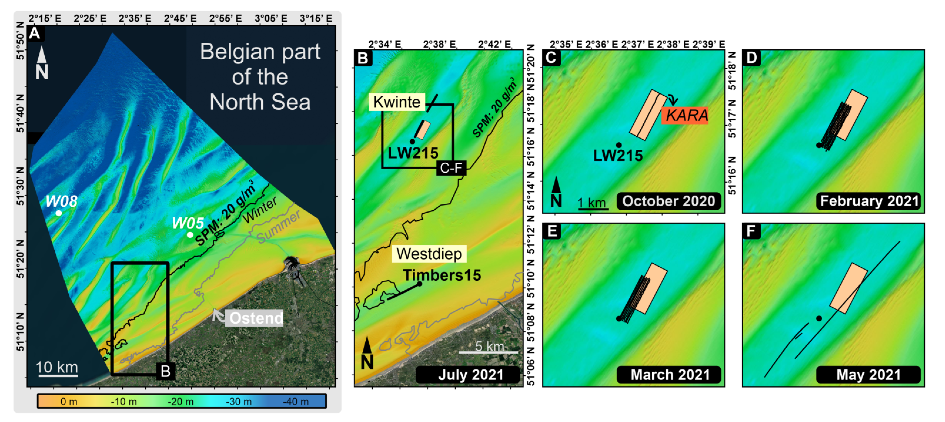
2. Study Area

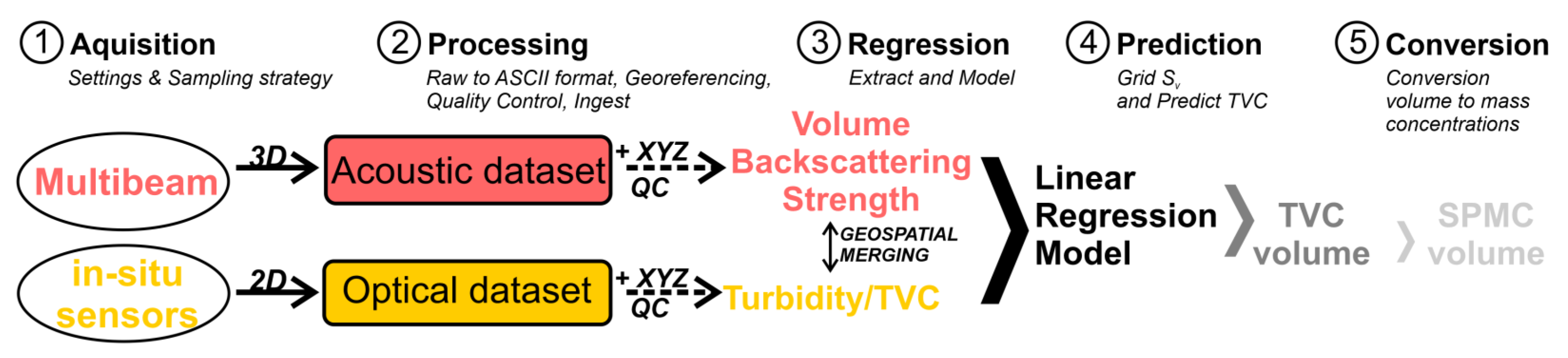
3. Materials and Methods
3.1. Data Acquisition
3.1.1. MBES–System and Settings
3.1.2. In Situ Sensor Toolbox: Settings and Deployment
3.1.3. Sensor Sensitivity
3.1.4. Sampling Strategy
3.2. Data Processing
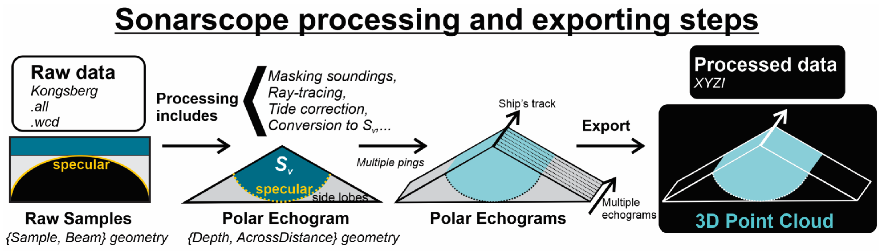
3.2.1. MBES Data
3.2.2. In-Situ Sensor Data
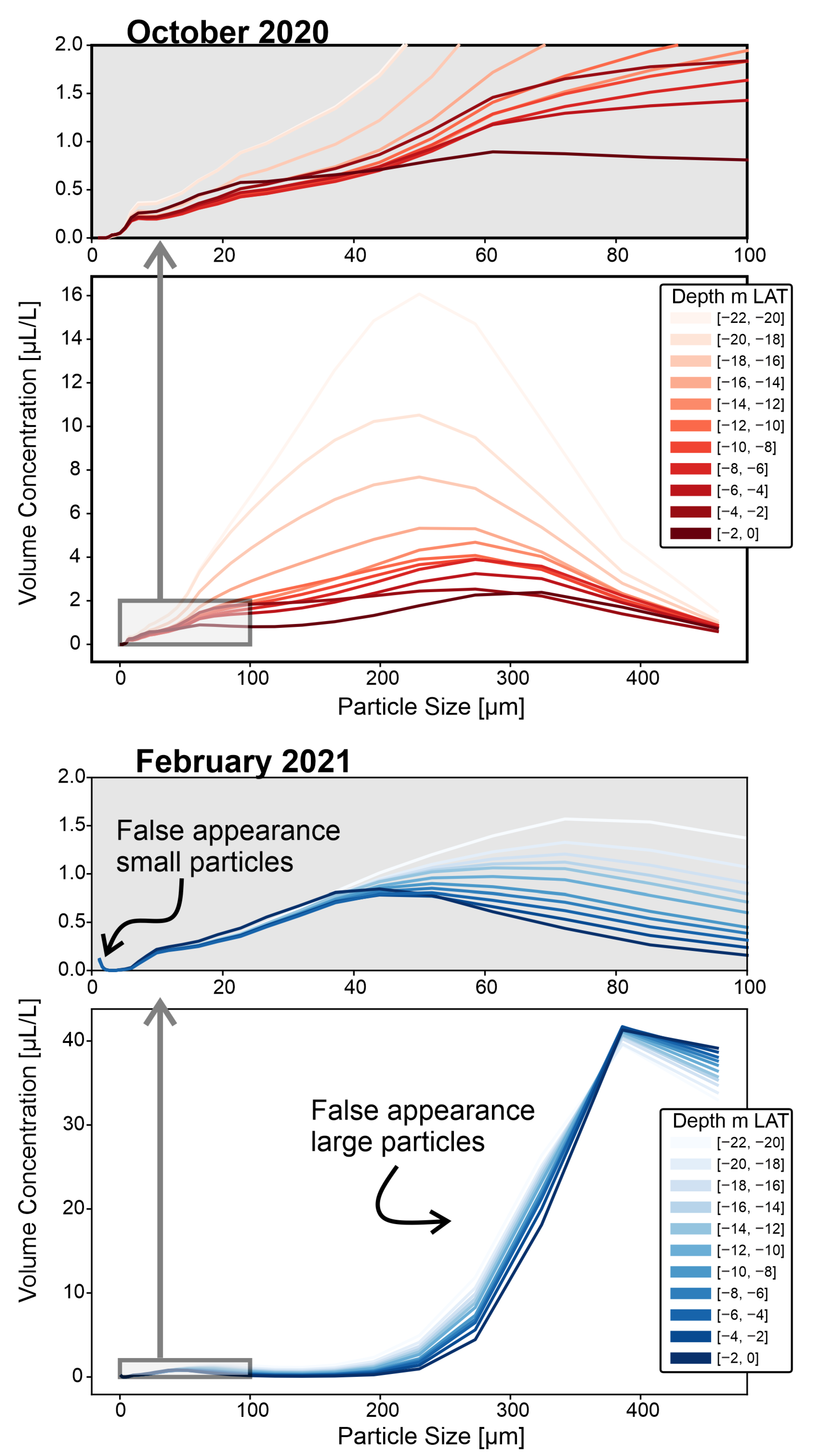
- During the February and March 2021 campaigns, the raw LISST scattering intensity data displayed an abnormal spiky pattern, especially the first six rings, which is characteristic for optical misalignment (Appendix B). The TVC values, which normally reflect sizes between 1–500 µm, were therefore recalculated to 2.42–180 µm (February 2021 campaign) and 1–180 µm (March 2021 campaign).
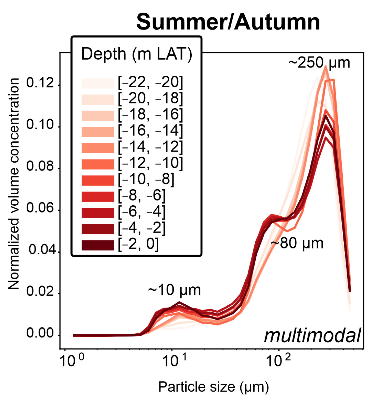
- Besides the particle concentration, particle sizes might also affect the scattering and absorption behavior, e.g., [17]. Hence, additional grain-size parameters were calculated based on the LISST’s particle size distribution, including the mass division diameter D50 value. Finally, as flocculation in coastal areas is a transient process, subjected to varying turbulent shear stresses, the (multimodal) particle size distribution actually consists of different particle populations. Therefore, TVC (in µL/L) was recalculated for four size ranges: TVC1–3 µm, TVC3–20 µm, TVC20–200 µm, TVC200–500 µm, which were assumed to represent primary particles, flocculi, microflocs, and macroflocs, respectively [10,90].
- As the depths of the acoustic Sv datasets were corrected for the tides and transformed into depth LAT within SonarScope, the same tide correction and transformation needs to be applied to the in situ sensor track. Therefore, we calculated the corrected LAT water depths of the LISST using the continuous RTK signal of the ship, which was smoothed (Butterworth filter; low-pass normalized cut-off frequency: 1/200; order: 2).
3.3. Data Analysis
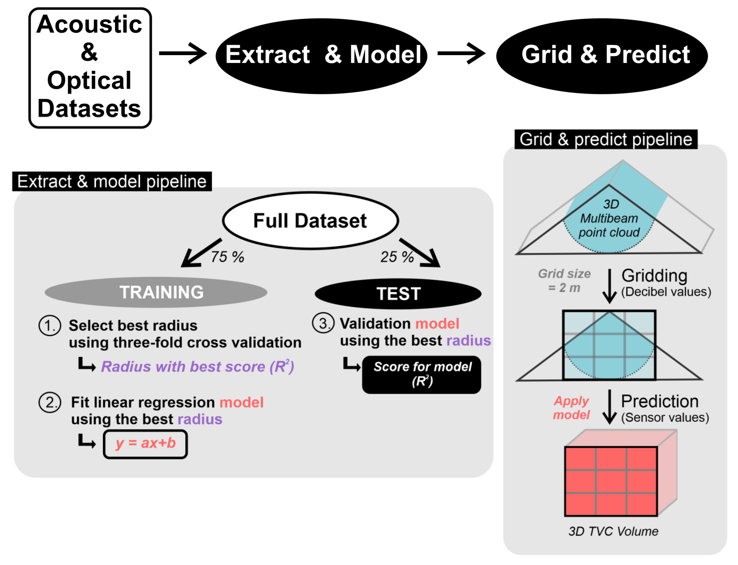
3.3.1. Regression and Prediction Analysis
3.3.2. Conversion to the Mass Concentrations
4. Results
4.1. Linear Regression Models
4.2. SPMC Volumes
5. Discussion
5.1. In Situ Sensor Datasets
5.2. Evaluation of the Linear Regression Models
5.3. Evaluation of the SPMC Volumes
5.4. Evaluation of the Sources of Uncertainty and Error
6. Lessons Learned and Outlook
6.1. Survey Strategy
6.2. MBES Water Column Processing
6.3. Statistical Modeling
6.4. Target Ambiguity
7. Conclusions
Supplementary Materials
Author Contributions
Funding
Data Availability Statement
Acknowledgments
Conflicts of Interest
Appendix A

| CAMPAIGNS | DATE | RAW MBES DATA | PROCESSED MBES DATA | IN-SITU SENSOR TOOLBOX | SURVEY AREA (STATIONS) |
|---|---|---|---|---|---|
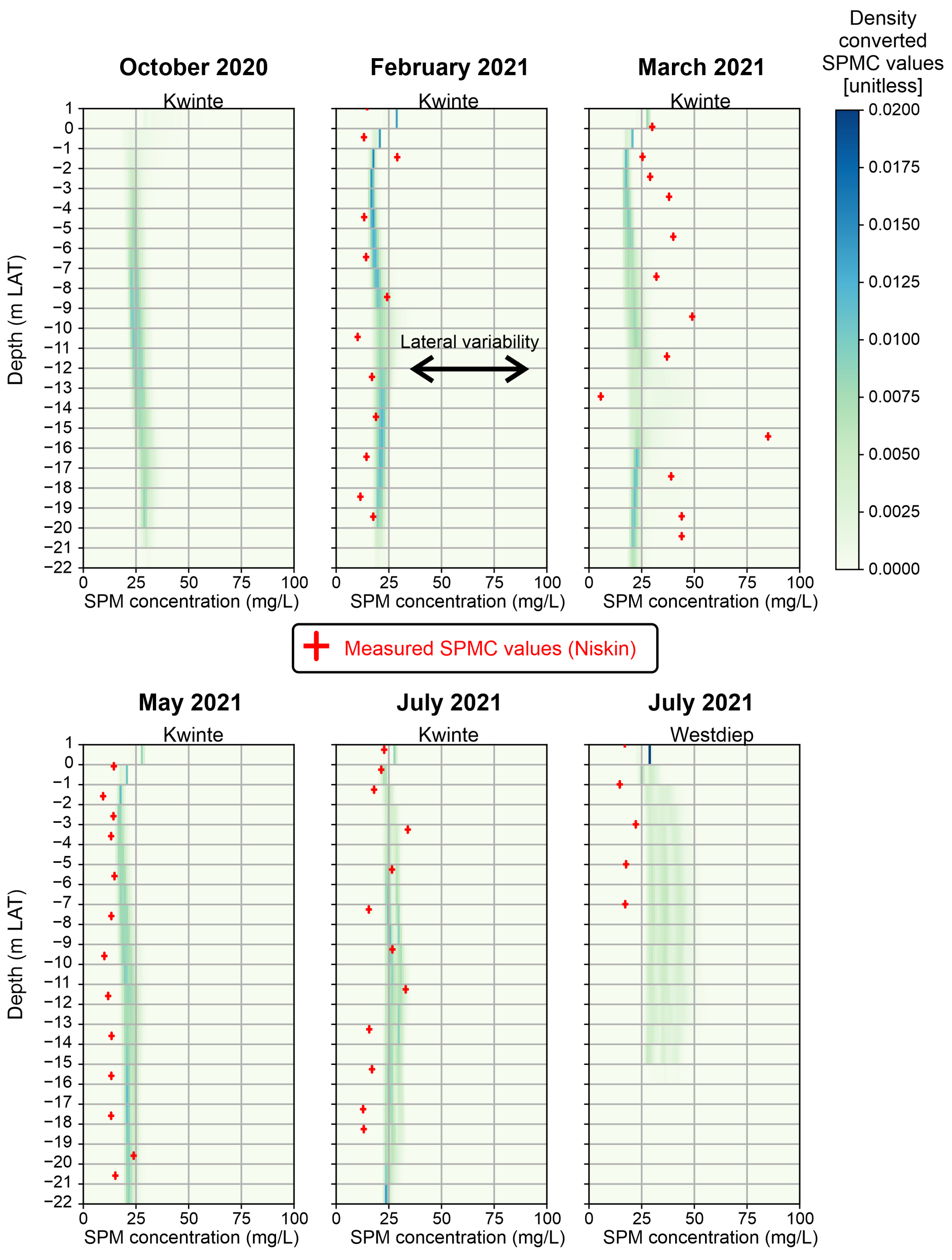
| OCTOBER 2020 20-690 | 5 October 2020 | 13.2 GB | 163 GB | LISST, OBS | Kwinte |
| FEBRUARY 2021 21-092 | 4 February 2021 | 90.4 GB | 1216 GB | LISST, (OBS), Niskin | Kwinte (LW215) |
| MARCH 2021 21-160 | 1 March 2021 | 62.7 GB | 594 GB | LISST, OBS, Niskin | Kwinte (LW215) |
| MAY 2021 21-430 | 28 May 2021 | 33.3 GB | 382 GB | LISST, Niskin | Kwinte (LW215) |
| JULY 2021 21-550 | 9 July 2021 | 23.3 GB | 188 GB | LISST, Niskin | Kwinte (LW215) Westdiep (Timbers 15) |
Appendix B
Appendix C
Appendix C.1. Uncertainties Related to the Regression Analyses
Appendix C.1.1. Extraction and Modeling
Appendix C.1.2. Gridding and Prediction
Appendix C.2. Uncertainties Related to the Conversion of TVC to SPMC

| SPMC (in mg/L) | October 2020 20-690 | February 2021 21-092 | March 2021 21-160 | May 2021 21-430 | July 2021 21-550_KW | July 2021 21-550_WD | |
|---|---|---|---|---|---|---|---|
| SPMC (1–500 µm) | lower limit | 6.617 | 5.058 | 5.713 | 5.213 | 6.518 | 8.816 |
| SPMC (1–500 µm) | mean | 27.179 | 20.775 | 23.466 | 21.411 | 26.769 | 36.213 |
| SPMC (1–500 µm) | upper limit | 70.398 | 53.812 | 60.781 | 55.457 | 69.337 | 93.811 |
| SPMC (1–3 µm) | lower limit | 0.006 | 0.012 | 0.010 | 0.011 | 0.006 | 0.003 |
| SPMC (1–3 µm) | mean | 0.067 | 0.129 | 0.106 | 0.119 | 0.066 | 0.034 |
| SPMC (1–3 µm) | upper limit | 0.410 | 0.790 | 0.649 | 0.728 | 0.403 | 0.212 |
| SPMC (3–20 µm) | lower limit | 0.804 | 0.490 | 0.629 | 0.516 | 0.766 | 1.340 |
| SPMC (3–20 µm) | mean | 2.823 | 1.718 | 2.205 | 1.810 | 2.689 | 4.702 |
| SPMC (3–20 µm) | upper limit | 6.673 | 4.061 | 5.213 | 4.278 | 6.357 | 11.116 |
| SPMC (20–200 µm) | lower limit | 0.500 | 0.344 | 0.411 | 0.359 | 0.487 | 0.742 |
| SPMC (20–200 µm) | mean | 2.325 | 1.599 | 1.911 | 1.666 | 2.261 | 3.449 |
| SPMC (20–200 µm) | upper limit | 7.281 | 5.008 | 5.986 | 5.217 | 7.083 | 10.803 |
| SPMC (200–500 µm) | lower limit | 0.025 | 0.024 | 0.024 | 0.024 | 0.025 | 0.027 |
| SPMC (200–500 µm) | mean | 0.231 | 0.219 | 0.224 | 0.221 | 0.230 | 0.244 |
| SPMC (200–500 µm) | upper limit | 1.427 | 1.356 | 1.385 | 1.364 | 1.424 | 1.507 |
References
- Kirk, J.T.O. Effects of suspensoids (turbidity) on penetration of solar radiation in aquatic ecosystems. Hydrobiologia 1985, 125, 195–208. [Google Scholar] [CrossRef]
- Gray, J.R.; Gartner, J.W. Technological advances in suspended-sediment surrogate monitoring. Water Resour. Res. 2009, 45, W00D29. [Google Scholar] [CrossRef]
- Capuzzo, E.; Lynam, C.P.; Barry, J.; Stephens, D.; Forster, R.M.; Greenwood, N.; McQuatters-Gollop, A.; Silva, T.; van Leeuwen, S.M.; Engelhard, G.H. A decline in primary production in the North Sea over 25 years, associated with reductions in zooplankton abundance and fish stock recruitment. Glob. Chang. Biol. 2018, 24, e352–e364. [Google Scholar] [CrossRef] [PubMed]
- Capuzzo, E.; Stephens, D.; Silva, T.; Barry, J.; Forster, R.M. Decrease in water clarity of the southern and central North Sea during the 20th century. Glob. Chang. Biol. 2015, 21, 2206–2214. [Google Scholar] [CrossRef] [PubMed]
- Lunt, J.; Smee, D.L. Turbidity alters estuarine biodiversity and species composition. ICES J. Mar. Sci. 2019, 77, 379–387. [Google Scholar] [CrossRef]
- Eisma, D.; Kalf, J. Distribution, organic content and particle size of suspended matter in the north sea. Neth. J. Sea Res. 1987, 21, 265–285. [Google Scholar] [CrossRef]
- Fettweis, M. Uncertainty of excess density and settling velocity of mud flocs derived from in situ measurements. Estuar. Coast. Shelf Sci. 2008, 78, 426–436. [Google Scholar] [CrossRef]
- Fettweis, M.; Baeye, M. Seasonal variation in concentration, size, and settling velocity of muddy marine flocs in the benthic boundary layer. J. Geophys. Res. Ocean. 2015, 120, 5648–5667. [Google Scholar] [CrossRef]
- Fettweis, M.; Lee, B.J. Spatial and Seasonal Variation of Biomineral Suspended Particulate Matter Properties in High-Turbid Nearshore and Low-Turbid Offshore Zones. Water 2017, 9, 694. [Google Scholar] [CrossRef]
- Fettweis, M.; Baeye, M.; Van der Zande, D.; Van den Eynde, D.; Joon Lee, B. Seasonality of floc strength in the southern North Sea. J. Geophys. Res. Ocean. 2014, 119, 1911–1926. [Google Scholar] [CrossRef]
- Fettweis, M.; Schartau, M.; Desmit, X.; Lee, B.J.; Terseleer, N.; Zande, D.V.d.; Riethmüller, R. Organic Matter Composition of Biomineral Flocs and its Influence on Suspended Particulate Matter Dynamics along a Nearshore to Offshore Transect. Earth Space Sci. Open Arch. 2022, 127, e2021JG006332. [Google Scholar] [CrossRef]
- Rai, A.K.; Kumar, A. Continuous measurement of suspended sediment concentration: Technological advancement and future outlook. Measurement 2015, 76, 209–227. [Google Scholar] [CrossRef]
- Ouillon, S. Why and How Do We Study Sediment Transport? Focus on Coastal Zones and Ongoing Methods. Water 2018, 10, 390. [Google Scholar] [CrossRef]
- Felix, D.; Albayrak, I.; Boes, R.M. In-situ investigation on real-time suspended sediment measurement techniques: Turbidimetry, acoustic attenuation, laser diffraction (LISST) and vibrating tube densimetry. Int. J. Sediment Res. 2018, 33, 3–17. [Google Scholar] [CrossRef]
- Rymszewicz, A.; O’Sullivan, J.J.; Bruen, M.; Turner, J.N.; Lawler, D.M.; Conroy, E.; Kelly-Quinn, M. Measurement differences between turbidity instruments, and their implications for suspended sediment concentration and load calculations: A sensor inter-comparison study. J. Environ. Manag. 2017, 199, 99–108. [Google Scholar] [CrossRef] [PubMed]
- Osborne, P.D.; Vincent, C.E.; Greenwood, B. Measurement of suspended sand concentrations in the nearshore: Field intercomparison of optical and acoustic backscatter sensors. Cont. Shelf Res. 1994, 14, 159–174. [Google Scholar] [CrossRef]
- Haalboom, S.; de Stigter, H.; Duineveld, G.; van Haren, H.; Reichart, G.-J.; Mienis, F. Suspended particulate matter in a submarine canyon (Whittard Canyon, Bay of Biscay, NE Atlantic Ocean): Assessment of commonly used instruments to record turbidity. Mar. Geol. 2021, 434, 106439. [Google Scholar] [CrossRef]
- Lin, J.; He, Q.; Guo, L.; van Prooijen, B.C.; Wang, Z.B. An integrated optic and acoustic (IOA) approach for measuring suspended sediment concentration in highly turbid environments. Mar. Geol. 2020, 421, 106062. [Google Scholar] [CrossRef]
- Winter, C.; Becker, M.; Ernstsen, V.B.; Hebbeln, D.; Port, A.; Bartholomä, A.; Flemming, B.; Lunau, M. In-situ observation of aggregate dynamics in a tidal channel using acoustics, laser diffraction and optics. J. Coast. Res. 2007, 1173–1177. [Google Scholar]
- Gartner, J.W. Estimating suspended solids concentrations from backscatter intensity measured by acoustic Doppler current profiler in San Francisco Bay, California. Mar. Geol. 2004, 211, 169–187. [Google Scholar] [CrossRef]
- Erikson, L.H.; Wright, S.A.; Elias, E.; Hanes, D.M.; Schoellhamer, D.H.; Largier, J. The use of modeling and suspended sediment concentration measurements for quantifying net suspended sediment transport through a large tidally dominated inlet. Mar. Geol. 2013, 345, 96–112. [Google Scholar] [CrossRef]
- Meslard, F.; Bourrin, F.; Many, G.; Kerhervé, P. Suspended particle dynamics and fluxes in an Arctic fjord (Kongsfjorden, Svalbard). Estuar. Coast. Shelf Sci. 2018, 204, 212–224. [Google Scholar] [CrossRef]
- Pawlak, G.; Moline, M.A.; Terrill, E.J.; Colin, P.L. Hydrodynamic influences on acoustical and optical backscatter in a fringing reef environment. J. Geophys. Res. Ocean. 2017, 122, 322–335. [Google Scholar] [CrossRef]
- Baeye, M.; Fettweis, M. In situ observations of suspended particulate matter plumes at an offshore wind farm, southern North Sea. Geo-Mar. Lett. 2015, 35, 247–255. [Google Scholar] [CrossRef]
- O’Connor, T.P. A Wider Look at the Risk of Ocean Disposal of Dredged Material. Mar. Pollut. Bull. 1999, 38, 760–761. [Google Scholar] [CrossRef]
- Lednicka, B.; Kubacka, M.; Freda, W.; Haule, K.; Dembska, G.; Galer-Tatarowicz, K.; Pazikowska-Sapota, G. Water Turbidity and Suspended Particulate Matter Concentration at Dredged Material Dumping Sites in the Southern Baltic. Sensors 2022, 22, 8049. [Google Scholar] [CrossRef] [PubMed]
- Eleveld, M.A.; Pasterkamp, R.; van der Woerd, H.J.; Pietrzak, J.D. Remotely sensed seasonality in the spatial distribution of sea-surface suspended particulate matter in the southern North Sea. Estuar. Coast. Shelf Sci. 2008, 80, 103–113. [Google Scholar] [CrossRef]
- El Serafy, G.Y.; Eleveld, M.A.; Blaas, M.; van Kessel, T.; Aguilar, S.G.; Van der Woerd, H.J. Improving the description of the suspended particulate matter concentrations in the southern North Sea through assimilating remotely sensed data. Ocean Sci. J. 2011, 46, 179. [Google Scholar] [CrossRef]
- Dogliotti, A.I.; Ruddick, K.G.; Nechad, B.; Doxaran, D.; Knaeps, E. A single algorithm to retrieve turbidity from remotely-sensed data in all coastal and estuarine waters. Remote Sens. Environ. 2015, 156, 157–168. [Google Scholar] [CrossRef]
- Baeye, M.; Fettweis, M.; Voulgaris, G.; Van Lancker, V. Sediment mobility in response to tidal and wind-driven flows along the Belgian inner shelf, southern North Sea. Ocean Dyn. 2011, 61, 611–622. [Google Scholar] [CrossRef]
- Fettweis, M.; Nechad, B.; Van den Eynde, D. An estimate of the suspended particulate matter (SPM) transport in the southern North Sea using SeaWiFS images, in situ measurements and numerical model results. Cont. Shelf Res. 2007, 27, 1568–1583. [Google Scholar] [CrossRef]
- Vanlede, J.; Dujardin, A.; Fettweis, M.; Van Hoestenberghe, T.; Martens, C. Mud dynamics in the Port of Zeebrugge. Ocean Dyn. 2019, 69, 1085–1099. [Google Scholar] [CrossRef]
- Van Lancker, V.; Baeye, M. Wave Glider Monitoring of Sediment Transport and Dredge Plumes in a Shallow Marine Sandbank Environment. PLoS ONE 2015, 10, e0128948. [Google Scholar] [CrossRef] [PubMed]
- Thorne, P.D.; Hurther, D. An overview on the use of backscattered sound for measuring suspended particle size and concentration profiles in non-cohesive inorganic sediment transport studies. Cont. Shelf Res. 2014, 73, 97–118. [Google Scholar] [CrossRef]
- Fromant, G.; Floc’h, F.; Lebourges-Dhaussy, A.; Jourdin, F.; Perrot, Y.; Le Dantec, N.; Delacourt, C. In Situ Quantification of the Suspended Load of Estuarine Aggregates from Multifrequency Acoustic Inversions. J. Atmos. Ocean. Technol. 2017, 34, 1625–1643. [Google Scholar] [CrossRef]
- Crawford, A.M.; Hay, A.E. Determining suspended sand size and concentration from multifrequency acoustic backscatter. J. Acoust. Soc. Am. 1993, 94, 3312–3324. [Google Scholar] [CrossRef]
- Holdaway, G.P.; Thorne, P.D.; Flatt, D.; Jones, S.E.; Prandle, D. Comparison between ADCP and transmissometer measurements of suspended sediment concentration. Cont. Shelf Res. 1999, 19, 421–441. [Google Scholar] [CrossRef]
- Moore, S.A.; Le Coz, J.; Hurther, D.; Paquier, A. On the application of horizontal ADCPs to suspended sediment transport surveys in rivers. Cont. Shelf Res. 2012, 46, 50–63. [Google Scholar] [CrossRef]
- Sheng, J.; Hay, A.E. An examination of the spherical scatterer approximation in aqueous suspensions of sand. J. Acoust. Soc. Am. 1988, 83, 598–610. [Google Scholar] [CrossRef]
- Thorne, P.D.; Meral, R. Formulations for the scattering properties of suspended sandy sediments for use in the application of acoustics to sediment transport processes. Cont. Shelf Res. 2008, 28, 309–317. [Google Scholar] [CrossRef]
- MacDonald, I.T.; Vincent, C.E.; Thorne, P.D.; Moate, B.D. Acoustic scattering from a suspension of flocculated sediments. J. Geophys. Res. Ocean. 2013, 118, 2581–2594. [Google Scholar] [CrossRef]
- Thorne, P.D.; MacDonald, I.T.; Vincent, C.E. Modelling acoustic scattering by suspended flocculating sediments. Cont. Shelf Res. 2014, 88, 81–91. [Google Scholar] [CrossRef]
- Ha, H.K.; Maa, J.P.Y.; Park, K.; Kim, Y.H. Estimation of high-resolution sediment concentration profiles in bottom boundary layer using pulse-coherent acoustic Doppler current profilers. Mar. Geol. 2011, 279, 199–209. [Google Scholar] [CrossRef]
- Sassi, M.G.; Hoitink, A.J.F.; Vermeulen, B. Impact of sound attenuation by suspended sediment on ADCP backscatter calibrations. Water Resour. Res. 2012, 48, W09520. [Google Scholar] [CrossRef]
- Sahin, C.; Safak, I.; Hsu, T.-J.; Sheremet, A. Observations of suspended sediment stratification from acoustic backscatter in muddy environments. Mar. Geol. 2013, 336, 24–32. [Google Scholar] [CrossRef]
- Filizola, N.; Guyot, J.L. The use of Doppler technology for suspended sediment discharge determination in the River Amazon/L’utilisation des techniques Doppler pour la détermination du transport solide de l’Amazone. Hydrol. Sci. J. 2004, 49, 143–153. [Google Scholar] [CrossRef]
- Venditti, J.G.; Domarad, N.; Church, M.; Rennie, C.D. The gravel-sand transition: Sediment dynamics in a diffuse extension. J. Geophys. Res. Earth Surf. 2015, 120, 943–963. [Google Scholar] [CrossRef]
- Hage, S.; Cartigny, M.J.B.; Sumner, E.J.; Clare, M.A.; Hughes Clarke, J.E.; Talling, P.J.; Lintern, D.G.; Simmons, S.M.; Silva Jacinto, R.; Vellinga, A.J.; et al. Direct Monitoring Reveals Initiation of Turbidity Currents From Extremely Dilute River Plumes. Geophys. Res. Lett. 2019, 46, 11310–11320. [Google Scholar] [CrossRef]
- Guerrero, M.; Szupiany, R.N.; Amsler, M. Comparison of acoustic backscattering techniques for suspended sediments investigation. Flow Meas. Instrum. 2011, 22, 392–401. [Google Scholar] [CrossRef]
- Simmons, S.M.; Parsons, D.R.; Best, J.L.; Orfeo, O.; Lane, S.N.; Kostaschuk, R.; Hardy, R.J.; West, G.; Malzone, C.; Marcus, J.; et al. Monitoring Suspended Sediment Dynamics Using MBES. J. Hydraul. Eng. 2010, 136, 45–49. [Google Scholar] [CrossRef]
- Best, J.; Simmons, S.; Parsons, D.; Oberg, K.; Czuba, J.; Malzone, C. A new methodology for the quantitative visualization of coherent flow structures in alluvial channels using multibeam echo-sounding (MBES). Geophys. Res. Lett. 2010, 37, L06405. [Google Scholar] [CrossRef]
- O’Neill, F.G.; Simmons, S.M.; Parsons, D.R.; Best, J.L.; Copland, P.J.; Armstrong, F.; Breen, M.; Summerbell, K. Monitoring the generation and evolution of the sediment plume behind towed fishing gears using a multibeam echosounder. ICES J. Mar. Sci. 2013, 70, 892–903. [Google Scholar] [CrossRef]
- Simmons, S.M.; Parsons, D.R.; Best, J.L.; Oberg, K.A.; Czuba, J.A.; Keevil, G.M. An evaluation of the use of a multibeam echo-sounder for observations of suspended sediment. Appl. Acoust. 2017, 126, 81–90. [Google Scholar] [CrossRef]
- Fromant, G.; Le Dantec, N.; Perrot, Y.; Floc’h, F.; Lebourges-Dhaussy, A.; Delacourt, C. Suspended sediment concentration field quantified from a calibrated MultiBeam EchoSounder. Appl. Acoust. 2021, 180, 108107. [Google Scholar] [CrossRef]
- Lurton, X. An Introduction to Underwater Acoustics: Principles and Applications; Springer: Berlin/Heidelberg, Germany, 2002; p. 680. [Google Scholar]
- Colbo, K.; Ross, T.; Brown, C.; Weber, T. A review of oceanographic applications of water column data from multibeam echosounders. Estuar. Coast. Shelf Sci. 2014, 145, 41–56. [Google Scholar] [CrossRef]
- Innangi, S.; Bonanno, A.; Tonielli, R.; Gerlotto, F.; Innangi, M.; Mazzola, S. High resolution 3-D shapes of fish schools: A new method to use the water column backscatter from hydrographic MultiBeam Echo Sounders. Appl. Acoust. 2016, 111, 148–160. [Google Scholar] [CrossRef]
- Urban, P.; Köser, K.; Greinert, J. Processing of multibeam water column image data for automated bubble/seep detection and repeated mapping. Limnol. Oceanogr. Methods 2017, 15, 1–21. [Google Scholar] [CrossRef]
- Westley, K.; Plets, R.; Quinn, R.; McGonigle, C.; Sacchetti, F.; Dale, M.; McNeary, R.; Clements, A. Optimising protocols for high-definition imaging of historic shipwrecks using multibeam echosounder. Archaeol. Anthropol. Sci. 2019, 11, 3629–3645. [Google Scholar] [CrossRef]
- Lowie, N. Evaluation of the Detection and Quantification of Sediment Plumes Caused by Dredging Activities Using a Multibeam Echosounder. Master’s Thesis, Ghent University, Flanders, Belgium, 2017. [Google Scholar]
- Roche, M.; Degrendele, K.; Vrignaud, C.; Loyer, S.; Le Bas, T.; Augustin, J.-M.; Lurton, X. Control of the repeatability of high frequency multibeam echosounder backscatter by using natural reference areas. Mar. Geophys. Res. 2018, 39, 89–104. [Google Scholar] [CrossRef]
- Acoustic Reference Area Kwinte (Maritime and Coastal Services-Flemish Hydrography). Available online: https://www.agentschapmdk.be/nl/akoestische-referentiezone-kwinte (accessed on 4 April 2023).
- Montereale-Gavazzi, G.; Roche, M.; Degrendele, K.; Lurton, X.; Terseleer, N.; Baeye, M.; Francken, F.; Van Lancker, V. Insights into the Short-Term Tidal Variability of Multibeam Backscatter from Field Experiments on Different Seafloor Types. Geosciences 2019, 9, 34. [Google Scholar] [CrossRef]
- Bathymetry Data (Maritime and Coastal Services-Flemish Hydrography). Available online: https://bathy.agentschapmdk.be/spatialfusionviewer/mapViewer/map.action (accessed on 4 April 2023).
- Mills, B.; Little, A. A High-resolution Aerial System of a New Type. Aust. J. Phys. 1953, 6, 272–278. [Google Scholar] [CrossRef]
- Agrawal, Y.C.; Pottsmith, H.C. Instruments for particle size and settling velocity observations in sediment transport. Mar. Geol. 2000, 168, 89–114. [Google Scholar] [CrossRef]
- SequoiaScientific. LISST-200X Particle Size Analyzer User’s Manual Version 2.35. 2022. Available online: https://www.sequoiasci.com/wp-content/uploads/2016/02/LISST-200X_Users_Manual_v2_35.pdf (accessed on 30 October 2021).
- Praet, N.; Vandorpe, T.; Ollevier, A.; Dierssen, H. TIMBERS in-situ sensor dataset. Mar. Data Arch. 2022. [Google Scholar] [CrossRef]
- Fugate, D.C.; Friedrichs, C.T. Determining concentration and fall velocity of estuarine particle populations using ADV, OBS and LISST. Cont. Shelf Res. 2002, 22, 1867–1886. [Google Scholar] [CrossRef]
- Downing, J. Twenty-five years with OBS sensors: The good, the bad, and the ugly. Cont. Shelf Res. 2006, 26, 2299–2318. [Google Scholar] [CrossRef]
- Haalboom, S.; de Stigter, H.C.; Mohn, C.; Vandorpe, T.; Smit, M.; de Jonge, L.; Reichart, G.-J. Monitoring of a sediment plume produced by a deep-sea mining test in shallow water, Málaga Bight, Alboran Sea (southwestern Mediterranean Sea). Mar. Geol. 2023, 456, 106971. [Google Scholar] [CrossRef]
- Hatcher, A.; Hill, P.; Grant, J. Optical backscatter of marine flocs. J. Sea Res. 2001, 46, 1–12. [Google Scholar] [CrossRef]
- Pearson, S.G.; Verney, R.; van Prooijen, B.C.; Tran, D.; Hendriks, E.C.M.; Jacquet, M.; Wang, Z.B. Characterizing the Composition of Sand and Mud Suspensions in Coastal and Estuarine Environments Using Combined Optical and Acoustic Measurements. J. Geophys. Res. Oceans 2021, 126, e2021JC017354. [Google Scholar] [CrossRef]
- Medwin, H.; Clay, C.S. Fundamentals of Acoustical Oceanography; Academic Press: San Diego, CA, USA, 1998; p. 712. [Google Scholar]
- Salehi, M.; Strom, K. Using velocimeter signal to noise ratio as a surrogate measure of suspended mud concentration. Cont. Shelf Res. 2011, 31, 1020–1032. [Google Scholar] [CrossRef]
- Lohrmann, A.N.A. Monitoring Sediment Concentration with acoustic backscattering instruments. Nortek Tech. Note 2001, 3, 5. [Google Scholar]
- Agrawal, Y.C.; Whitmire, A.; Mikkelsen, O.A.; Pottsmith, H.C. Light scattering by random shaped particles and consequences on measuring suspended sediments by laser diffraction. J. Geophys. Res. Oceans 2008, 113, C04023. [Google Scholar] [CrossRef]
- Andrews, S.; Nover, D.; Schladow, S.G. Using laser diffraction data to obtain accurate particle size distributions: The role of particle composition. Limnol. Oceanogr. Methods 2010, 8, 507–526. [Google Scholar] [CrossRef]
- Andrews, S.W.; Nover, D.M.; Reuter, J.E.; Schladow, S.G. Limitations of laser diffraction for measuring fine particles in oligotrophic systems: Pitfalls and potential solutions. Water Resour. Res. 2011, 47, W05523. [Google Scholar] [CrossRef]
- Felix, D.; Albayrak, I.; Boes, R.M. Laboratory investigation on measuring suspended sediment by portable laser diffractometer (LISST) focusing on particle shape. Geo-Mar. Lett. 2013, 33, 485–498. [Google Scholar] [CrossRef]
- Augustin, J.-M. SonarScope Software. SEANOE. 2022. Available online: https://www.seanoe.org/data/00766/87777/ (accessed on 4 April 2023).
- Lamarche, G.; Lurton, X. Recommendations for improved and coherent acquisition and processing of backscatter data from seafloor-mapping sonars. Mar. Geophys. Res. 2018, 39, 5–22. [Google Scholar] [CrossRef]
- Foote, K.G.; Chu, D.; Hammar, T.R.; Baldwin, K.C.; Mayer, L.A.; Hufnagle, L.C.; Jech, J.M. Protocols for calibrating multibeam sonar. J. Acoust. Soc. Am 2005, 117, 2013–2027. [Google Scholar] [CrossRef] [PubMed]
- Perrot, Y.; Brehmer, P.; Roudaut, G.; Gerstoft, P.; Josse, E. Efficient multibeam sonar calibration and performance evaluation. Int. J. Innov. Res. Sci. Eng. Technol. 2014, 3, 808–820. [Google Scholar]
- Hughes Clarke, J.E. Applications of Multibeam Water Column Imaging for Hydrographic Survey. Hydrogr. J. 2006, 120, 3–15. [Google Scholar]
- Schimel, A.C.G.; Brown, C.J.; Ierodiaconou, D. Automated Filtering of Multibeam Water-Column Data to Detect Relative Abundance of Giant Kelp (Macrocystis pyrifera). Remote Sens. 2020, 12, 1371. [Google Scholar] [CrossRef]
- Manning, C. Entwine—Point Cloud Organization for Massive Datasets. Available online: https://entwine.io (accessed on 4 April 2023).
- Schütz, M. Potree: WebGL Point Cloud Viewer for Large Datasets. Available online: http://potree.org (accessed on 4 April 2023).
- Collart, T.; Praet, N. Data and Python Scripts Used for the TIMBERS Project. 2023. Available online: https://zenodo.org/records/8423005 (accessed on 4 April 2023).
- Lee, B.J.; Fettweis, M.; Toorman, E.; Molz, F.J. Multimodality of a particle size distribution of cohesive suspended particulate matters in a coastal zone. J. Geophys. Res. Ocean. 2012, 117. [Google Scholar] [CrossRef]
- Fettweis, M.; Baeye, M.; Lee, B.J.; Chen, P.; Yu, J.C.S. Hydro-meteorological influences and multimodal suspended particle size distributions in the Belgian nearshore area (southern North Sea). Geo-Mar. Lett. 2012, 32, 123–137. [Google Scholar] [CrossRef]
- PDALContributors. PDAL Point Data Abstraction Library. Available online: https://pdal.io/en/2.6.0/ (accessed on 4 April 2023).
- DaskDevelopmentTeam. Dask: Library for Dynamic Task Scheduling. Available online: https://dask.org (accessed on 4 April 2023).
- Fettweis, M.; Riethmüller, R.; Verney, R.; Becker, M.; Backers, J.; Baeye, M.; Chapalain, M.; Claeys, S.; Claus, J.; Cox, T.; et al. Uncertainties associated with in situ high-frequency long-term observations of suspended particulate matter concentration using optical and acoustic sensors. Prog. Oceanogr. 2019, 178, 102162. [Google Scholar] [CrossRef]
- Fall, K.A.; Friedrichs, C.T.; Massey, G.M.; Bowers, D.G.; Smith, S.J. The Importance of Organic Content to Fractal Floc Properties in Estuarine Surface Waters: Insights From Video, LISST, and Pump Sampling. J. Geophys. Res. Ocean. 2021, 126, e2020JC016787. [Google Scholar] [CrossRef]
- Kranenburg, C. The fractal structure of cohesive sediment aggregates. Estuar. Coast. Shelf Sci. 1994, 39, 451–460. [Google Scholar] [CrossRef]
- Winterwerp, J.C. A simple model for turbulence induced flocculation of cohesive sediment. J. Hydraul. Res. 1998, 36, 309–326. [Google Scholar] [CrossRef]
- Jago, C.F.; Jones, S.E.; Sykes, P.; Rippeth, T. Temporal variation of suspended particulate matter and turbulence in a high energy, tide-stirred, coastal sea: Relative contributions of resuspension and disaggregation. Cont. Shelf Res. 2006, 26, 2019–2028. [Google Scholar] [CrossRef]
- Praet, N.; Collart, T. 3D Volumes of Suspended Particulate Matter in the Belgian Part of the North Sea. 2023. Available online: https://zenodo.org/records/8013207 (accessed on 4 April 2023).
- Sahin, C.; Ozturk, M.; Aydogan, B. Acoustic doppler velocimeter backscatter for suspended sediment measurements: Effects of sediment size and attenuation. Appl. Ocean. Res. 2020, 94, 101975. [Google Scholar] [CrossRef]
- Rouhnia, M.; Keyvani, A.; Strom, K. Do changes in the size of mud flocs affect the acoustic backscatter values recorded by a Vector ADV? Cont. Shelf Res. 2014, 84, 84–92. [Google Scholar] [CrossRef]
- Vergne, A.; Berni, C.; Le Coz, J.; Tencé, F. Acoustic Backscatter and Attenuation Due to River Fine Sediments: Experimental Evaluation of Models and Inversion Methods. Water Resour. Res. 2021, 57, e2021WR029589. [Google Scholar] [CrossRef]
- Pedocchi, F.; Mosquera, R. Acoustic backscatter and attenuation of a flocculated cohesive sediment suspension. Cont. Shelf Res. 2022, 240, 104719. [Google Scholar] [CrossRef]
- Vincent, C.E.; MacDonald, I.T. A flocculi model for the acoustic scattering from flocs. Cont. Shelf Res. 2015, 104, 15–24. [Google Scholar] [CrossRef]
- Fettweis, M.; Francken, F.; Pison, V.; Van den Eynde, D. Suspended particulate matter dynamics and aggregate sizes in a high turbidity area. Mar. Geol. 2006, 235, 63–74. [Google Scholar] [CrossRef]
- Fettweis, M.P.; Nechad, B. Evaluation of in situ and remote sensing sampling methods for SPM concentrations, Belgian continental shelf (southern North Sea). Ocean Dyn. 2011, 61, 157–171. [Google Scholar] [CrossRef]
- Lanzoni, J.C.; Weber, T.C. Calibration of multibeam echo sounders: A comparison between two methodologies. Proc. Mtgs. Acoust. 2012, 17. [Google Scholar] [CrossRef]
- Mikkelsen, O.; Pejrup, M. The use of a LISST-100 laser particle sizer for in-situ estimates of floc size, density and settling velocity. Geo-Mar. Lett. 2001, 20, 187–195. [Google Scholar] [CrossRef]
- Moate, B.D.; Thorne, P.D. Interpreting acoustic backscatter from suspended sediments of different and mixed mineralogical composition. Cont. Shelf Res. 2012, 46, 67–82. [Google Scholar] [CrossRef]
- Wilson, G.W.; Hay, A.E. Acoustic backscatter inversion for suspended sediment concentration and size: A new approach using statistical inverse theory. Cont. Shelf Res. 2015, 106, 130–139. [Google Scholar] [CrossRef]
- Hawkins, A.D.; Roberts, L.; Cheesman, S. Responses of free-living coastal pelagic fish to impulsive sounds. J. Acoust. Soc. Am. 2014, 135, 3101–3116. [Google Scholar] [CrossRef]
- Francisco, F.; Bender, A.; Sundberg, J. Use of multibeam imaging sonar for observation of marine mammals and fish on a marine renewable energy site. PLoS ONE 2022, 17, e0275978. [Google Scholar] [CrossRef]
- Nilsson, L.A.F.; Thygesen, U.H.; Lundgren, B.; Nielsen, B.F.; Nielsen, J.R.; Beyer, J.E. Vertical migration and dispersion of sprat (Sprattus sprattus) and herring (Clupea harengus) schools at dusk in the Baltic Sea. Aquat. Living Resour. 2003, 16, 317–324. [Google Scholar] [CrossRef]
- Chen, K.; Zhou, M.; Zhong, Y.; Waniek, J.J.; Shan, C.; Zhang, Z. Effects of Mixing and Stratification on the Vertical Distribution and Size Spectrum of Zooplankton on the Shelf and Slope of the Northern South China Sea. Front. Mar. Sci. 2022, 9, 870021. [Google Scholar] [CrossRef]
- Lezama-Ochoa, A.; Ballón, M.; Woillez, M.; Grados, D.; Irigoien, X.; Bertrand, A. Spatial patterns and scale-dependent relationships between macrozooplankton and fish in the Bay of Biscay: An acoustic study. Mar. Ecol. Prog. Ser. 2011, 439, 151–168. [Google Scholar] [CrossRef]
- Neukermans, G.; Reynolds, R.A.; Stramski, D. Contrasting inherent optical properties and particle characteristics between an under-ice phytoplankton bloom and open water in the Chukchi Sea. Deep. Sea Res. Part II Top. Stud. Oceanogr. 2014, 105, 59–73. [Google Scholar] [CrossRef]
- Clavano, W.; Boss, E.; Karp-Boss, L. Inherent Optical Properties of Non-Spherical Marine-Like Particles—From Theory To Observation. Oceanogr. Mar. Biol. 2007, 45, 1–38. [Google Scholar] [CrossRef]


| Size Range (in µm) | North Sea SPM | Density ρa (kg/m3) | Lower Limit ρa (kg/m3) | Upper Limit ρa (kg/m3) |
|---|---|---|---|---|
| 1–3 | primary particles | 2329 | 1000 | 3175 |
| 3–20 | flocculi | 758 | 319 | 1213 |
| 20–200 | microflocs | 93 | 32 | 183 |
| 200–500 | macroflocs | 16 | 1 | 38 |
| 1–500 | SPM | 614 | 259 | 922 |
| Yi | TVC (1–500 µm) | TVC (1–3 µm) | TVC (3–20 µm) | TVC (20–200 µm) | TVC (200–500 µm) | Optical Turbidity (NTU) |
|---|---|---|---|---|---|---|
| Observations n | 6529 | 784 | 6529 | 6529 | 6529 | 12024 |
| α | 3.635 | −6.499 | 4.134 | 4.134 | 1.524 | 5.979 |
| β | 0.029 | −0.073 | 0.053 | 0.040 | 0.006 | 0.074 |
| Standard error α | 0.029 | 0.561 | 0.020 | 0.025 | 0.054 | 0.090 |
| Standard error β | 0.000 | 0.008 | 0.000 | 0.000 | 0.001 | 0.001 |
| Standard error of regression | 0.121 | 0.331 | 0.086 | 0.103 | 0.211 | 0.290 |
| p value β | 0.000 | 0.000 | 0.000 | 0.000 | 0.000 | 0.000 |
| Adjusted R2 (test dataset) | 0.439 | 0.195 | 0.843 | 0.651 | 0.007 | 0.211 |
| Best radius (m) | 5 | 5 | 5 | 4 | 1 | 5 |
Disclaimer/Publisher’s Note: The statements, opinions and data contained in all publications are solely those of the individual author(s) and contributor(s) and not of MDPI and/or the editor(s). MDPI and/or the editor(s) disclaim responsibility for any injury to people or property resulting from any ideas, methods, instructions or products referred to in the content. |
© 2023 by the authors. Licensee MDPI, Basel, Switzerland. This article is an open access article distributed under the terms and conditions of the Creative Commons Attribution (CC BY) license (https://creativecommons.org/licenses/by/4.0/).
Share and Cite
Praet, N.; Collart, T.; Ollevier, A.; Roche, M.; Degrendele, K.; De Rijcke, M.; Urban, P.; Vandorpe, T. The Potential of Multibeam Sonars as 3D Turbidity and SPM Monitoring Tool in the North Sea. Remote Sens. 2023, 15, 4918. https://doi.org/10.3390/rs15204918
Praet N, Collart T, Ollevier A, Roche M, Degrendele K, De Rijcke M, Urban P, Vandorpe T. The Potential of Multibeam Sonars as 3D Turbidity and SPM Monitoring Tool in the North Sea. Remote Sensing. 2023; 15(20):4918. https://doi.org/10.3390/rs15204918
Chicago/Turabian StylePraet, Nore, Tim Collart, Anouk Ollevier, Marc Roche, Koen Degrendele, Maarten De Rijcke, Peter Urban, and Thomas Vandorpe. 2023. "The Potential of Multibeam Sonars as 3D Turbidity and SPM Monitoring Tool in the North Sea" Remote Sensing 15, no. 20: 4918. https://doi.org/10.3390/rs15204918