


Utilizing Hyperspectral Reflectance and Machine Learning Algorithms for Non-Destructive Estimation of Chlorophyll Content in Citrus Leaves


 ,
,  and
and
Abstract
:1. Introduction
2. Materials and Methods
2.1. Experimental Site and Experimental Design
2.2. Measurement of the Hyperspectral Data
2.3. Measurement of Leaf Chlorophyll Content
2.4. Extraction of Spectral Parameters
2.5. Dimension Reduction and Parameter Selection
2.6. Linear Regression Analysis
2.7. Machine Learning Algorithms
3. Results
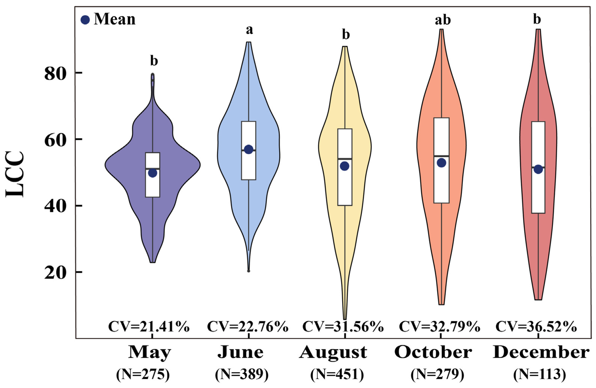
3.1. Statistics of Measured LCC
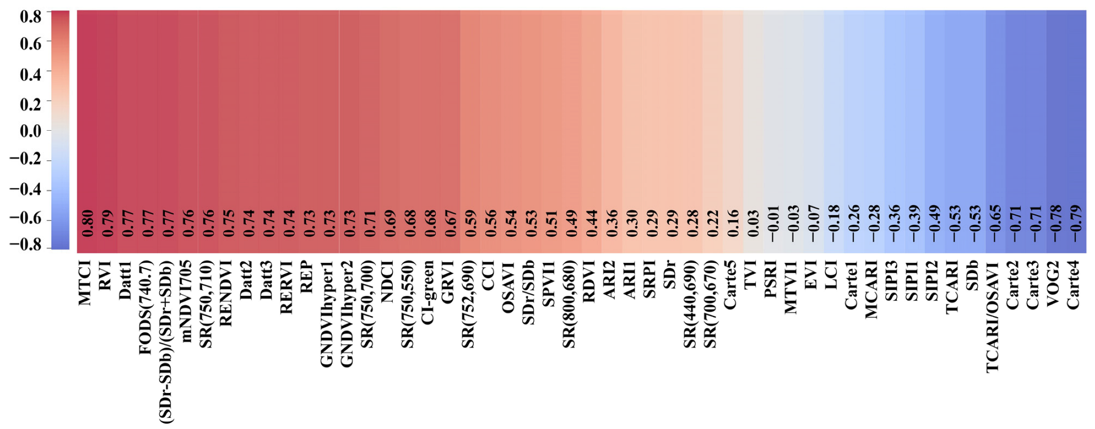
3.2. Parameters Selection
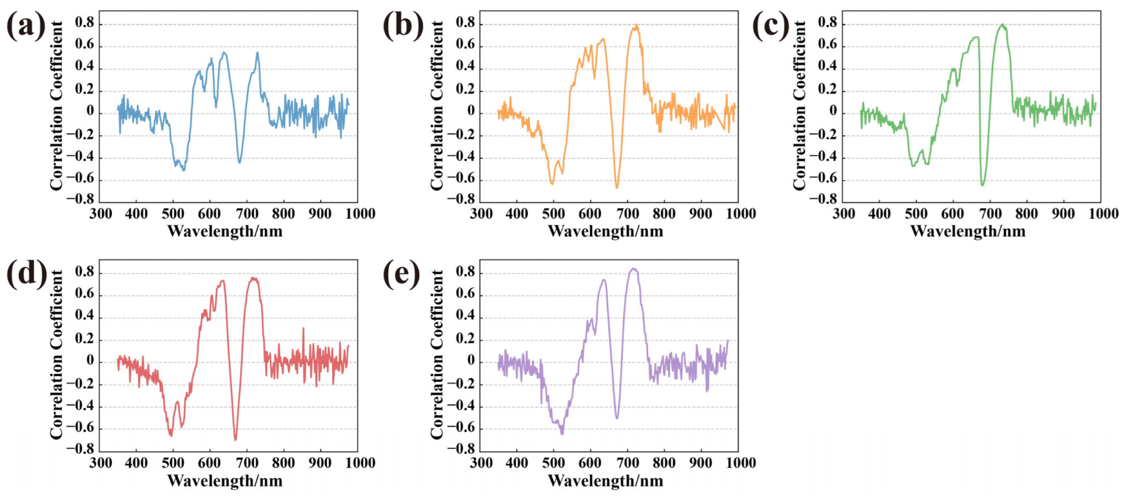
3.3. Univariate Linear Regression
3.4. Multivariate Linear Regression
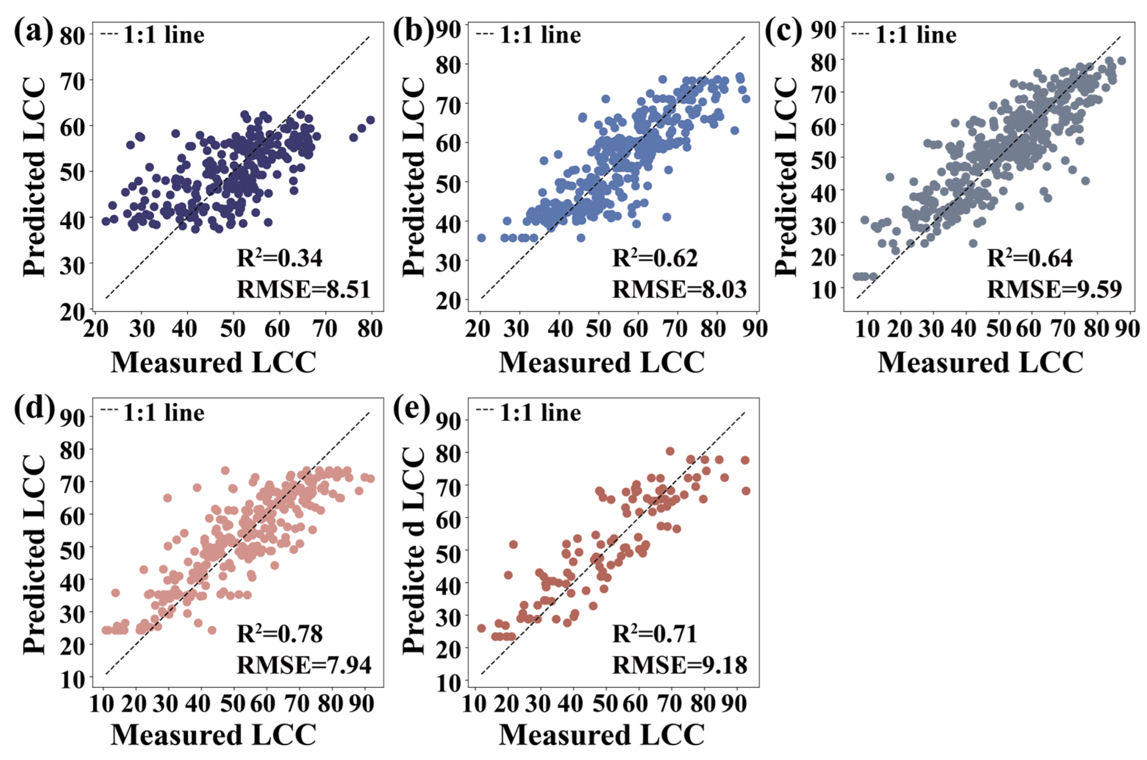
3.5. Machine Learning Algorithms
4. Discussion
4.1. Linear Regression Analysis of the Spectral Parameters for LCC Estimation
4.2. Performance Evaluation of Machine Learning Algorithms for LCC Estimation
4.3. Exploring Future Prospects in Citrus Chlorophyll Research
5. Conclusions
Author Contributions
Funding
Data Availability Statement
Conflicts of Interest
References
- Peng, Y.; Nguy-Robertson, A.; Arkebauer, T.; Gitelson, A. Assessment of Canopy Chlorophyll Content Retrieval in Maize and Soybean: Implications of Hysteresis on the Development of Generic Algorithms. Remote Sens. 2017, 9, 226. [Google Scholar] [CrossRef]
- Evans, J.R. Photosynthesis and Nitrogen Relationships in Leaves of C3 Plants. Oecologia 1989, 78, 9–19. [Google Scholar] [CrossRef]
- Luo, J.; Zhou, J.-J.; Masclaux-Daubresse, C.; Wang, N.; Wang, H.; Zheng, B. Morphological and Physiological Responses to Contrasting Nitrogen Regimes in Populus Cathayana Is Linked to Resources Allocation and Carbon/Nitrogen Partition. Environ. Exp. Bot. 2019, 162, 247–255. [Google Scholar] [CrossRef]
- Porcar-Castell, A.; Tyystjärvi, E.; Atherton, J.; Van Der Tol, C.; Flexas, J.; Pfündel, E.E.; Moreno, J.; Frankenberg, C.; Berry, J.A. Linking Chlorophyll a Fluorescence to Photosynthesis for Remote Sensing Applications: Mechanisms and Challenges. J. Exp. Bot. 2014, 65, 4065–4095. [Google Scholar] [CrossRef]
- Croft, H.; Chen, J.M.; Luo, X.; Bartlett, P.; Chen, B.; Staebler, R.M. Leaf Chlorophyll Content as a Proxy for Leaf Photosynthetic Capacity. Glob. Chang. Biol. 2017, 23, 3513–3524. [Google Scholar] [CrossRef]
- Sage, R.F.; Pearcy, R.W.; Seemann, J.R. The Nitrogen Use Efficiency of C3 and C4 Plants: III. Leaf Nitrogen Effects on the Activity of Carboxylating Enzymes in Chenopodium album (L.) and Amaranthus retroflexus (L.). Plant Physiol. 1987, 85, 355–359. [Google Scholar] [CrossRef]
- Luo, J.; Zhou, J.; Li, H.; Shi, W.; Polle, A.; Lu, M.; Sun, X.; Luo, Z.-B. Global Poplar Root and Leaf Transcriptomes Reveal Links between Growth and Stress Responses under Nitrogen Starvation and Excess. Tree Physiol. 2015, 35, 1283–1302. [Google Scholar] [CrossRef]
- Qiao, L.; Tang, W.; Gao, D.; Zhao, R.; An, L.; Li, M.; Sun, H.; Song, D. UAV-Based Chlorophyll Content Estimation by Evaluating Vegetation Index Responses under Different Crop Coverages. Comput. Electron. Agric. 2022, 196, 106775. [Google Scholar] [CrossRef]
- Aasen, H.; Honkavaara, E.; Lucieer, A.; Zarco-Tejada, P. Quantitative Remote Sensing at Ultra-High Resolution with UAV Spectroscopy: A Review of Sensor Technology, Measurement Procedures, and Data Correction Workflows. Remote Sens. 2018, 10, 1091. [Google Scholar] [CrossRef]
- Ta, N.; Chang, Q.; Zhang, Y. Estimation of Apple Tree Leaf Chlorophyll Content Based on Machine Learning Methods. Remote Sens. 2021, 13, 3902. [Google Scholar] [CrossRef]
- Zhou, J.-J.; Zhang, Y.-H.; Han, Z.-M.; Liu, X.-Y.; Jian, Y.-F.; Hu, C.-G.; Dian, Y.-Y. Evaluating the Performance of Hyperspectral Leaf Reflectance to Detect Water Stress and Estimation of Photosynthetic Capacities. Remote Sens. 2021, 13, 2160. [Google Scholar] [CrossRef]
- Gamon, J.A.; Somers, B.; Malenovský, Z.; Middleton, E.M.; Rascher, U.; Schaepman, M.E. Assessing Vegetation Function with Imaging Spectroscopy. Surv. Geophys. 2019, 40, 489–513. [Google Scholar] [CrossRef]
- Zhang, Y.; Hui, J.; Qin, Q.; Sun, Y.; Zhang, T.; Sun, H.; Li, M. Transfer-Learning-Based Approach for Leaf Chlorophyll Content Estimation of Winter Wheat from Hyperspectral Data. Remote Sens. Environ. 2021, 267, 112724. [Google Scholar] [CrossRef]
- Zarco-Tejada, P.J.; González-Dugo, M.V.; Fereres, E. Seasonal Stability of Chlorophyll Fluorescence Quantified from Airborne Hyperspectral Imagery as an Indicator of Net Photosynthesis in the Context of Precision Agriculture. Remote Sens. Environ. 2016, 179, 89–103. [Google Scholar] [CrossRef]
- Datt, B. Remote Sensing of Chlorophyll a, Chlorophyll b, Chlorophyll a+b, and Total Carotenoid Content in Eucalyptus Leaves. Remote Sens. Environ. 1998, 66, 111–121. [Google Scholar] [CrossRef]
- Yamashita, H.; Sonobe, R.; Hirono, Y.; Morita, A.; Ikka, T. Dissection of Hyperspectral Reflectance to Estimate Nitrogen and Chlorophyll Contents in Tea Leaves Based on Machine Learning Algorithms. Sci. Rep. 2020, 10, 17360. [Google Scholar] [CrossRef]
- Poobalasubramanian, M.; Park, E.-S.; Faqeerzada, M.A.; Kim, T.; Kim, M.S.; Baek, I.; Cho, B.-K. Identification of Early Heat and Water Stress in Strawberry Plants Using Chlorophyll-Fluorescence Indices Extracted via Hyperspectral Images. Sensors 2022, 22, 8706. [Google Scholar] [CrossRef]
- Zheng, Y.; Zhang, T.; Zhang, J.; Chen, X.; Shen, X. Influence of smooth, 1st derivative and baseline correction on the near-infrared spectrum analysis with PLS. Spectrosc. Spectr. Anal. 2004, 24, 1546–1548. [Google Scholar]
- Zhao, T.; Komatsuzaki, M.; Okamoto, H.; Sakai, K. Cover Crop Nutrient and Biomass Assessment System Using Portable Hyperspectral Camera and Laser Distance Sensor. Eng. Agric. Environ. Food 2010, 3, 105–112. [Google Scholar] [CrossRef]
- Zhao, T.; Nakano, A.; Iwaski, Y.; Umeda, H. Application of Hyperspectral Imaging for Assessment of Tomato Leaf Water Status in Plant Factories. Appl. Sci. 2020, 10, 4665. [Google Scholar] [CrossRef]
- Turpie, K.R. Explaining the Spectral Red-Edge Features of Inundated Marsh Vegetation. J. Coast. Res. 2013, 290, 1111–1117. [Google Scholar] [CrossRef]
- Shah, S.H.; Angel, Y.; Houborg, R.; Ali, S.; McCabe, M.F. A Random Forest Machine Learning Approach for the Retrieval of Leaf Chlorophyll Content in Wheat. Remote Sens. 2019, 11, 920. [Google Scholar] [CrossRef]
- Cui, B.; Zhao, Q.; Huang, W.; Song, X.; Ye, H.; Zhou, X. A New Integrated Vegetation Index for the Estimation of Winter Wheat Leaf Chlorophyll Content. Remote Sens. 2019, 11, 974. [Google Scholar] [CrossRef]
- Zhu, W.; Sun, Z.; Yang, T.; Li, J.; Peng, J.; Zhu, K.; Li, S.; Gong, H.; Lyu, Y.; Li, B.; et al. Estimating Leaf Chlorophyll Content of Crops via Optimal Unmanned Aerial Vehicle Hyperspectral Data at Multi-Scales. Comput. Electron. Agric. 2020, 178, 105786. [Google Scholar] [CrossRef]
- Wang, J.; Chen, Y.; Chen, F.; Shi, T.; Wu, G. Wavelet-Based Coupling of Leaf and Canopy Reflectance Spectra to Improve the Estimation Accuracy of Foliar Nitrogen Concentration. Agric. For. Meteorol. 2018, 248, 306–315. [Google Scholar] [CrossRef]
- Wang, L.; Zhou, X.; Zhu, X.; Dong, Z.; Guo, W. Estimation of Biomass in Wheat Using Random Forest Regression Algorithm and Remote Sensing Data. Crop J. 2016, 4, 212–219. [Google Scholar] [CrossRef]
- Cavallo, D.P.; Cefola, M.; Pace, B.; Logrieco, A.F.; Attolico, G. Contactless and Non-Destructive Chlorophyll Content Prediction by Random Forest Regression: A Case Study on Fresh-Cut Rocket Leaves. Comput. Electron. Agric. 2017, 140, 303–310. [Google Scholar] [CrossRef]
- Liu, H.; Li, M.; Zhang, J.; Gao, D.; Sun, H.; Yang, L. Estimation of Chlorophyll Content in Maize Canopy Using Wavelet Denoising and SVR Method. Int. J. Agric. Biol. Eng. 2018, 11, 132–137. [Google Scholar] [CrossRef]
- Barman, U.; Sarmah, A.; Sahu, D.; Barman, G.G. Estimation of Tea Leaf Chlorophyll Using MLR, ANN, SVR, and KNN in Natural Light Condition. In Proceedings of the International Conference on Computing and Communication Systems; Maji, A.K., Saha, G., Das, S., Basu, S., Tavares, J.M.R.S., Eds.; Springer: Singapore, 2021; pp. 287–295. [Google Scholar]
- Narmilan, A.; Gonzalez, F.; Salgadoe, A.S.A.; Kumarasiri, U.W.L.M.; Weerasinghe, H.A.S.; Kulasekara, B.R. Predicting Canopy Chlorophyll Content in Sugarcane Crops Using Machine Learning Algorithms and Spectral Vegetation Indices Derived from UAV Multispectral Imagery. Remote Sens. 2022, 14, 1140. [Google Scholar] [CrossRef]
- Ma, R.; Tang, T.; Wang, X. Correlation Analysis of Citrus Chlorophyll Content based on Machine Learning. Sci. Technol. Innov. 2023, 72–75. [Google Scholar]
- Kong, W.; Huang, W.; Zhou, X.; Ye, H.; Dong, Y.; Casa, R. Off-Nadir Hyperspectral Sensing for Estimation of Vertical Profile of Leaf Chlorophyll Content within Wheat Canopies. Sensors 2017, 17, 2711. [Google Scholar] [CrossRef] [PubMed]
- Jin, X.; Li, Z.; Feng, H.; Xu, X.; Yang, G. Newly Combined Spectral Indices to Improve Estimation of Total Leaf Chlorophyll Content in Cotton. IEEE J. Sel. Top. Appl. Earth Obs. Remote Sens. 2014, 7, 4589–4600. [Google Scholar] [CrossRef]
- Jin, X.; Wang, K.; Xiao, C.; Diao, W.; Wang, F.; Chen, B.; Li, S. Comparison of Two Methods for Estimation of Leaf Total Chlorophyll Content Using Remote Sensing in Wheat. Field Crops Res. 2012, 135, 24–29. [Google Scholar] [CrossRef]
- Ali, A.; Imran, M. Remotely Sensed Real-Time Quantification of Biophysical and Biochemical Traits of Citrus (Citrus sinensis L.) Fruit Orchards—A Review. Sci. Hortic. 2021, 282, 110024. [Google Scholar] [CrossRef]
- Sari, M.; Sonmez, N.K.; Karaca, M. Relationship between Chlorophyll Content and Canopy Reflectance in Washington Navel Orange Trees (Citrus sinensis (L.) Osbeck). Pak. J. Bot. 2005, 37, 1093–1102. [Google Scholar]
- Osco, L.P.; Ramos, A.P.M.; Faita Pinheiro, M.M.; Moriya, É.A.S.; Imai, N.N.; Estrabis, N.; Ianczyk, F.; de Araújo, F.F.; Liesenberg, V.; de Castro Jorge, L.A.; et al. A Machine Learning Framework to Predict Nutrient Content in Valencia-Orange Leaf Hyperspectral Measurements. Remote Sens. 2020, 12, 906. [Google Scholar] [CrossRef]
- Gerhards, M.; Schlerf, M.; Mallick, K.; Udelhoven, T. Challenges and Future Perspectives of Multi-/Hyperspectral Thermal Infrared Remote Sensing for Crop Water-Stress Detection: A Review. Remote Sens. 2019, 11, 1240. [Google Scholar] [CrossRef]
- Li, F.; Wang, L.; Liu, J.; Wang, Y.; Chang, Q. Evaluation of Leaf N Concentration in Winter Wheat Based on Discrete Wavelet Transform Analysis. Remote Sens. 2019, 11, 1331. [Google Scholar] [CrossRef]
- Gitelson, A.A.; Merzlyak, M.N.; Chivkunova, O.B. Optical Properties and Nondestructive Estimation of Anthocyanin Content in Plant Leaves. Photochem. Photobiol. 2007, 74, 38–45. [Google Scholar] [CrossRef]
- Liang, L.; Qin, Z.; Zhao, S.; Di, L.; Zhang, C.; Deng, M.; Lin, H.; Zhang, L.; Wang, L.; Liu, Z. Estimating Crop Chlorophyll Content with Hyperspectral Vegetation Indices and the Hybrid Inversion Method. Int. J. Remote Sens. 2016, 37, 2923–2949. [Google Scholar] [CrossRef]
- Carter, G.A. Ratios of Leaf Reflectances in Narrow Wavebands as Indicators of Plant Stress. Int. J. Remote Sens. 1994, 15, 697–703. [Google Scholar] [CrossRef]
- Datt, B. A New Reflectance Index for Remote Sensing of Chlorophyll Content in Higher Plants: Tests Using Eucalyptus Leaves. J. Plant Physiol. 1999, 154, 30–36. [Google Scholar] [CrossRef]
- Huete, A.; Justice, C.; Liu, H. Development of Vegetation and Soil Indices for MODIS-EOS. Remote Sens. Environ. 1994, 49, 224–234. [Google Scholar] [CrossRef]
- Daughtry, C.S.T.; Walthall, C.L.; Kim, M.S.; de Colstoun, E.B.; McMurtrey, J.E. Estimating Corn Leaf Chlorophyll Concentration from Leaf and Canopy Reflectance. Remote Sens. Environ. 2000, 74, 229–239. [Google Scholar] [CrossRef]
- Haboudane, D.; Miller, J.R.; Pattey, E.; Zarco-Tejada, P.J.; Strachan, I.B. Hyperspectral Vegetation Indices and Novel Algorithms for Predicting Green LAI of Crop Canopies: Modeling and Validation in the Context of Precision Agriculture. Remote Sens. Environ. 2004, 90, 337–352. [Google Scholar] [CrossRef]
- Marshak, A.; Knyazikhin, Y.; Davis, A.B.; Wiscombe, W.J.; Pilewskie, P. Cloud-Vegetation Interaction: Use of Normalized Difference Cloud Index for Estimation of Cloud Optical Thickness. Geophys. Res. Lett. 2000, 27, 1695–1698. [Google Scholar] [CrossRef]
- Merzlyak, M.N.; Gitelson, A.A.; Chivkunova, O.B.; Rakitin, V.Y. Non-Destructive Optical Detection of Pigment Changes during Leaf Senescence and Fruit Ripening. Physiol. Plant. 1999, 106, 135–141. [Google Scholar] [CrossRef]
- Roujean, J.-L.; Breon, F.-M. Estimating PAR Absorbed by Vegetation from Bidirectional Reflectance Measurements. Remote Sens. Environ. 1995, 51, 375–384. [Google Scholar] [CrossRef]
- Clevers, J.G.P.W. Imaging Spectrometry in Agriculture—Plant Vitality and Yield Indicators. In Imaging Spectrometry—A Tool for Environmental Observations; Eurocourses: Remote Sensing; Hill, J., Mégier, J., Eds.; Springer: Dordrecht, The Netherlands, 1994; Volume 4, pp. 193–219. ISBN 978-0-7923-2965-7. [Google Scholar]
- Vincini, M.; Frazzi, E.; D’Alessio, P. Angular Dependence of Maize and Sugar Beet VIs from Directional CHRIS/Proba Data. In Proceedings of the 4th ESA CHRIS PROBA Workshop, ESRIN, Frascati, Italy, 19–21 September 2006. [Google Scholar]
- Penuelas, J.; Frederic, B.; Filella, I. Semi-Empirical Indices to Assess Carotenoids/Chlorophyll Alpha Ratio from Leaf Spectral Reflectance. Photosynthetica 1995, 31, 221–230. [Google Scholar]
- Lichtenthaler, H.K.; Lang, M.; Stober, F.; Sowinska, M.; Heisel, F.; Miehe, J.A. Detection of Photosynthetic Parameters and Vegetation Stress via a a New High Resolution Fluorescence Imaging-System. In Proceedings of the EARSeL, Basel, Switzerland, 4–6 September 1995; p. 103. [Google Scholar]
- McMurtrey, J.E.; Chappelle, E.W.; Kim, M.S.; Meisinger, J.J.; Corp, L.A. Distinguishing Nitrogen Fertilization Levels in Field Corn (Zea mays L.) with Actively Induced Fluorescence and Passive Reflectance Measurements. Remote Sens. Environ. 1994, 47, 36–44. [Google Scholar] [CrossRef]
- Gitelson, A.A.; Merzlyak, M.N. Remote Estimation of Chlorophyll Content in Higher Plant Leaves. Int. J. Remote Sens. 1997, 18, 2691–2697. [Google Scholar] [CrossRef]
- Zarco-Tejada, P.J.; Miller, J.R. Land Cover Mapping at BOREAS Using Red Edge Spectral Parameters from CASI Imagery. J. Geophys. Res. 1999, 104, 27921–27933. [Google Scholar] [CrossRef]
- Sims, D.A.; Gamon, J.A. Relationships between Leaf Pigment Content and Spectral Reflectance across a Wide Range of Species, Leaf Structures and Developmental Stages. Remote Sens. Environ. 2002, 81, 337–354. [Google Scholar] [CrossRef]
- Haboudane, D.; Miller, J.R.; Tremblay, N.; Zarco-Tejada, P.J.; Dextraze, L. Integrated Narrow-Band Vegetation Indices for Prediction of Crop Chlorophyll Content for Application to Precision Agriculture. Remote Sens. Environ. 2002, 81, 416–426. [Google Scholar] [CrossRef]
- Rondeaux, G.; Steven, M.; Baret, F. Optimization of Soil-Adjusted Vegetation Indices. Remote Sens. Environ. 1996, 55, 95–107. [Google Scholar] [CrossRef]
- Broge, N.H.; Leblanc, E. Comparing Prediction Power and Stability of Broadband and Hyperspectral Vegetation Indices for Estimation of Green Leaf Area Index and Canopy Chlorophyll Density. Remote Sens. Environ. 2001, 76, 156–172. [Google Scholar] [CrossRef]
- Datt, B. Remote Sensing of Water Content in Eucalyptus Leaves. Aust. J. Bot. 1999, 47, 909. [Google Scholar] [CrossRef]
- Blackburn, G.A. Spectral Indices for Estimating Photosynthetic Pigment Concentrations: A Test Using Senescent Tree Leaves. Int. J. Remote Sens. 1998, 19, 657–675. [Google Scholar] [CrossRef]
- Gitelson, A.A. Remote Estimation of Canopy Chlorophyll Content in Crops. Geophys. Res. Lett. 2005, 32, L08403. [Google Scholar] [CrossRef]
- Fitzgerald, G.; Rodriguez, D.; O’Leary, G. Measuring and Predicting Canopy Nitrogen Nutrition in Wheat Using a Spectral Index—The Canopy Chlorophyll Content Index (CCCI). Field Crops Res. 2010, 116, 318–324. [Google Scholar] [CrossRef]
- Dash, J.; Curran, P.J. The MERIS Terrestrial Chlorophyll Index. Int. J. Remote Sens. 2004, 25, 5403–5413. [Google Scholar] [CrossRef]
- Gitelson, A.A.; Keydan, G.P.; Merzlyak, M.N. Three-band Model for Noninvasive Estimation of Chlorophyll, Carotenoids, and Anthocyanin Contents in Higher Plant Leaves. Geophys. Res. Lett. 2006, 33, 2006GL026457. [Google Scholar] [CrossRef]
- Jordan, C.F. Derivation of Leaf-Area Index from Quality of Light on the Forest Floor. Ecology 1969, 50, 663–666. [Google Scholar] [CrossRef]
- Li, X.; Liu, G.; Yang, Y.; Zhao, C.; Yu, Q.; Song, S. Relationship Between Hyperspectral Parameters and Physiological and Biochemical Indexes of Flue-Cured Tobacco Leaves. Agric. Sci. China 2007, 6, 665–672. [Google Scholar] [CrossRef]
- Ying, X. An Overview of Overfitting and Its Solutions. J. Phys. Conf. Ser. 2019, 1168, 022022. [Google Scholar] [CrossRef]
- Fonti, V.; Belitser, E. Paper in Business Analytics Feature Selection Using LASSO; VU Amsterdam: Amsterdam, The Netherlands, 2017; Volume 30, pp. 1–25. [Google Scholar]
- Qi, Y. Random Forest for Bioinformatics. In Ensemble Machine Learning: Methods and Applications; Zhang, C., Ma, Y., Eds.; Springer: New York, NY, USA, 2012; pp. 307–323. ISBN 978-1-4419-9326-7. [Google Scholar]
- Zhang, C.; Denka, S.; Cooper, H.; Mishra, D.R. Quantification of Sawgrass Marsh Aboveground Biomass in the Coastal Everglades Using Object-Based Ensemble Analysis and Landsat Data. Remote Sens. Environ. 2018, 204, 366–379. [Google Scholar] [CrossRef]
- Smola, A.J.; Schölkopf, B. A Tutorial on Support Vector Regression. Stat. Comput. 2004, 14, 199–222. [Google Scholar] [CrossRef]
- Were, K.; Bui, D.T.; Dick, Ø.B.; Singh, B.R. A Comparative Assessment of Support Vector Regression, Artificial Neural Networks, and Random Forests for Predicting and Mapping Soil Organic Carbon Stocks across an Afromontane Landscape. Ecol. Indic. 2015, 52, 394–403. [Google Scholar] [CrossRef]
- Cho, M.A.; Skidmore, A.K. A New Technique for Extracting the Red Edge Position from Hyperspectral Data: The Linear Extrapolation Method. Remote Sens. Environ. 2006, 101, 181–193. [Google Scholar] [CrossRef]
- Guo, T.; Tan, C.; Li, Q.; Cui, G.; Li, H. Estimating Leaf Chlorophyll Content in Tobacco Based on Various Canopy Hyperspectral Parameters. J. Ambient Intell. Hum. Comput. 2019, 10, 3239–3247. [Google Scholar] [CrossRef]
- Zhang, X.; Sun, H.; Qiao, X.; Yan, X.; Feng, M.; Xiao, L.; Song, X.; Zhang, M.; Shafiq, F.; Yang, W.; et al. Hyperspectral Estimation of Canopy Chlorophyll of Winter Wheat by Using the Optimized Vegetation Indices. Comput. Electron. Agric. 2022, 193, 106654. [Google Scholar] [CrossRef]
- Shi, H.; Guo, J.; An, J.; Tang, Z.; Wang, X.; Li, W.; Zhao, X.; Jin, L.; Xiang, Y.; Li, Z.; et al. Estimation of Chlorophyll Content in Soybean Crop at Different Growth Stages Based on Optimal Spectral Index. Agronomy 2023, 13, 663. [Google Scholar] [CrossRef]
- Li, L.; Ren, T.; Ma, Y.; Wei, Q.; Wang, S.; Li, X.; Cong, R.; Liu, S.; Lu, J. Evaluating Chlorophyll Density in Winter Oilseed Rape (Brassica napus L.) Using Canopy Hyperspectral Red-Edge Parameters. Comput. Electron. Agric. 2016, 126, 21–31. [Google Scholar] [CrossRef]
- Zarco-Tejada, P.J.; Miller, J.R.; Morales, A.; Berjón, A.; Agüera, J. Hyperspectral Indices and Model Simulation for Chlorophyll Estimation in Open-Canopy Tree Crops. Remote Sens. Environ. 2004, 90, 463–476. [Google Scholar] [CrossRef]
- Bhadra, S.; Sagan, V.; Maimaitijiang, M.; Maimaitiyiming, M.; Newcomb, M.; Shakoor, N.; Mockler, T.C. Quantifying Leaf Chlorophyll Concentration of Sorghum from Hyperspectral Data Using Derivative Calculus and Machine Learning. Remote Sens. 2020, 12, 2082. [Google Scholar] [CrossRef]
- Angel, Y.; McCabe, M.F. Machine Learning Strategies for the Retrieval of Leaf-Chlorophyll Dynamics: Model Choice, Sequential Versus Retraining Learning, and Hyperspectral Predictors. Front. Plant Sci. 2022, 13, 722442. [Google Scholar] [CrossRef]
- An, G.; Xing, M.; He, B.; Liao, C.; Huang, X.; Shang, J.; Kang, H. Using Machine Learning for Estimating Rice Chlorophyll Content from In Situ Hyperspectral Data. Remote Sens. 2020, 12, 3104. [Google Scholar] [CrossRef]
- Maimaitijiang, M.; Sagan, V.; Sidike, P.; Daloye, A.M.; Erkbol, H.; Fritschi, F.B. Crop Monitoring Using Satellite/UAV Data Fusion and Machine Learning. Remote Sens. 2020, 12, 1357. [Google Scholar] [CrossRef]
- Liu, Y.; Zhang, Y.; Jiang, D.; Zhang, Z.; Chang, Q. Quantitative Assessment of Apple Mosaic Disease Severity Based on Hyperspectral Images and Chlorophyll Content. Remote Sens. 2023, 15, 2202. [Google Scholar] [CrossRef]


| NO. | Name | Explanation | Reference |
|---|---|---|---|
| 1 | Anthocyanin Reflectance Index 1 | ARI1 = 1/R550 − 1/R700 | [40] |
| 2 | Anthocyanin Reflectance Index 2 | ARI2 = R800(1/R550 − 1/R700) | [41] |
| 3 | Green Normalized Difference Vegetation Index hyper 1 | GNDVIhyper1 = (R750 − R550)/(R750 + R550) | [41] |
| 4 | Green Normalized Difference Vegetation Index hyper 2 | GNDVIhyper2 = (R800 − R550)/(R800 + R550) | [41] |
| 5 | Modified Normalized Difference Vegetation Index | mNDVI705 = (R750 − R705)/(R750 + R705 − 2R445) | [41] |
| 6 | Canopy Chlorophyll Index | CCI = (R777 − R747)/R673 | [41] |
| 7 | Vogelmann Index 2 | VOG2 = (R734 − R747)/(R715 + R726) | [41] |
| 8 | Carter1 | Carte1 = R695/R420 | [42] |
| 9 | Carter2 | Carte2 = R695/R760 | [42] |
| 10 | Carter3 | Carte3 = R605/R760 | [42] |
| 11 | Carter4 | Carte4 = R710/R760 | [42] |
| 12 | Carter5 | Carte5 = R695/R670 | [42] |
| 13 | Datt1 | Datt1 = (R850 − R710)/(R850 − R680) | [43] |
| 14 | Datt2 | Datt2 = R850/R710 | [43] |
| 15 | Datt3 | Datt3 = R754/R704 | [43] |
| 16 | Enhanced Vegetation Index | EVI = 2.5 × ((R800 − R670)/R800 − 6R670 − 7.5R475 + 1)) | [44] |
| 17 | Modified Chlorophyll Absorption in Reflectance Index | MCARI = ((R700 − R670) − 0.2 × (R700 − R550))(R700/R670) | [45] |
| 18 | Modified Triangular Vegetation Index 1 | MTVI1 = 1.2 × (1.2 × (R800 − R550) − 2.5 × (R670 − R550)) | [46] |
| 19 | Normalized Difference Cloud Index | NDCI = (R762 − R527)/(R762 + R527) | [47] |
| 20 | Plant Senescence Reflectance Index | PSRI = (R678 − R500)/R750 | [48] |
| 21 | Renormalized Difference Vegetation Index | RDVI = (R800 − R670)/ | [49] |
| 22 | Red-Edge Position Linear Interpolation | REP = 700 + 40 × ((R670 + R780)/2 − R700)/(R740 − R700) | [50] |
| 23 | Spectral Polygon Vegetation Index 1 | SPVI1 = 0.4 × 3.7 × (R800 − R670) − 1.2 × |R530 − R670| | [51] |
| 24 | Simple Ratio Pigment Index | SRPI = R430/R680 | [52] |
| 25 | Simple Ratio 440/690 | SR(440,690) = R440/R690 | [53] |
| 26 | Simple Ratio 700/670 | SR(700,670) = R700/R670 | [54] |
| 27 | Simple Ratio 750/550 | SR(750,550) = R750/R550 | [54] |
| 28 | Simple Ratio 750/700 | SR(750,700) = R750/R700 | [55] |
| 29 | Simple Ratio 750/710 | SR(750,710) = R750/R710 | [56] |
| 30 | Simple Ratio 752/690 | SR(752,690) = R752/R690 | [56] |
| 31 | Simple Ratio 800/680 | SR(800,680) = R800/R680 | [57] |
| 32 | Transformed Chlorophyll Absorption Ratio | TCARI = 3 × ((R700 − R670) − 0.2× (R700 − R550)(R700/R670)) | [58] |
| 33 | Optimized Soil Adjusted Vegetation Index | OSAVI = (1 + 0.16) × (R800 − R670)/(R800 + R670 + 0.16) | [59] |
| 34 | Transformed Chlorophyll Absorption in Reflectance Index/Optimized Soil Adjusted Vegetation Index | TCARI/OSAVI = | [41] |
| 35 | Triangular Vegetation Index | TVI = 0.5 × (120× (R750 − R550) − 200 × (R670 − R550)) | [60] |
| 36 | Leaf Chlorophyll Index | LCI = | [61] |
| 37 | Structure Intensive Pigment Index 1 | SIPI1 = (R800 − R445)/(R800 − R680) | [62] |
| 38 | Structure Intensive Pigment Index 2 | SIPI2 = (R800 − R505)/(R800 − R690) | [62] |
| 39 | Structure Intensive Pigment Index 3 | SIPI3 = (R800 − R470)/(R800 − R680) | [62] |
| 40 | Red-Edge Ratio Vegetation Index | RERVI = R840/R717 | [63] |
| 41 | Red-Edge Normalized Difference Vegetation Index | RENDVI = (R840 − R717)/(R840 + R717) | [64] |
| 42 | Green Ratio Vegetation Index | GRVI = R840/R560 | [63] |
| 43 | MERIS Terrestrial Chlorophyll Index | MTCI = (R753 − R708)/(R708 − R681) | [65] |
| 44 | Chlorophyll Index Green | CI-green = (R780/R550) − 1 | [66] |
| 45 | Ratio Vegetation Index | RVI = R765/R720 | [67] |
| 46 | FODS | First-order differential spectrum | [39] |
| 47 | SDr | First-order differential spectral integration in the wavelength range of 680~760 nm | [68] |
| 48 | SDb | First-order differential spectral integration in the wavelength range of 490~530 nm | [68] |
| 49 | SDr/SDb | Ratio of the red edge area to the blue edge area | [68] |
| 50 | (SDr − SDb)/(SDr + SDb) | Normalized value of the red edge area and the blue edge area | [68] |
| Growth Seasons | Models | R2 | RMSE | Parameter |
|---|---|---|---|---|
| May | y = 49.680 + 6.1210 × x1 | 0.20 | 8.88 | FODS (647.2) |
| June | y = 55.974 + 10.689 × x1 | 0.61 | 6.85 | Datt1 |
| August | y = 52.045 + 14.207 × x1 | 0.69 | 8.92 | MTCI |
| October | y = 52.131 − 14.277 × x1 | 0.66 | 8.81 | Carte4 |
| December | y = 50.612 + 15.170 × x1 | 0.72 | 9.72 | FODS (730.2) |
| Growth Seasons | Models | R2 | RMSE |
|---|---|---|---|
| May | y = 49.710 − 7.616 × x1 − 11.644 × x2 − 10.097 × x3 | 0.29 | 8.59 |
| June | y = 55.819 + 2.387 × x1 − 11.107 × x2 − 2.689 × x3 | 0.64 | 7.93 |
| August | y = 52.875 − 5.880 × x1 + 13.748 × x2 − 6.317 × x3 | 0.68 | 8.79 |
| October | y = 52.274 − 29.580 × x1 − 27.842 × x2 − 16.227 × x3 | 0.77 | 7.70 |
| December | y = 51.278 − 21.262 × x1 − 33.347 × x2 − 27.079 × x3 | 0.76 | 8.56 |
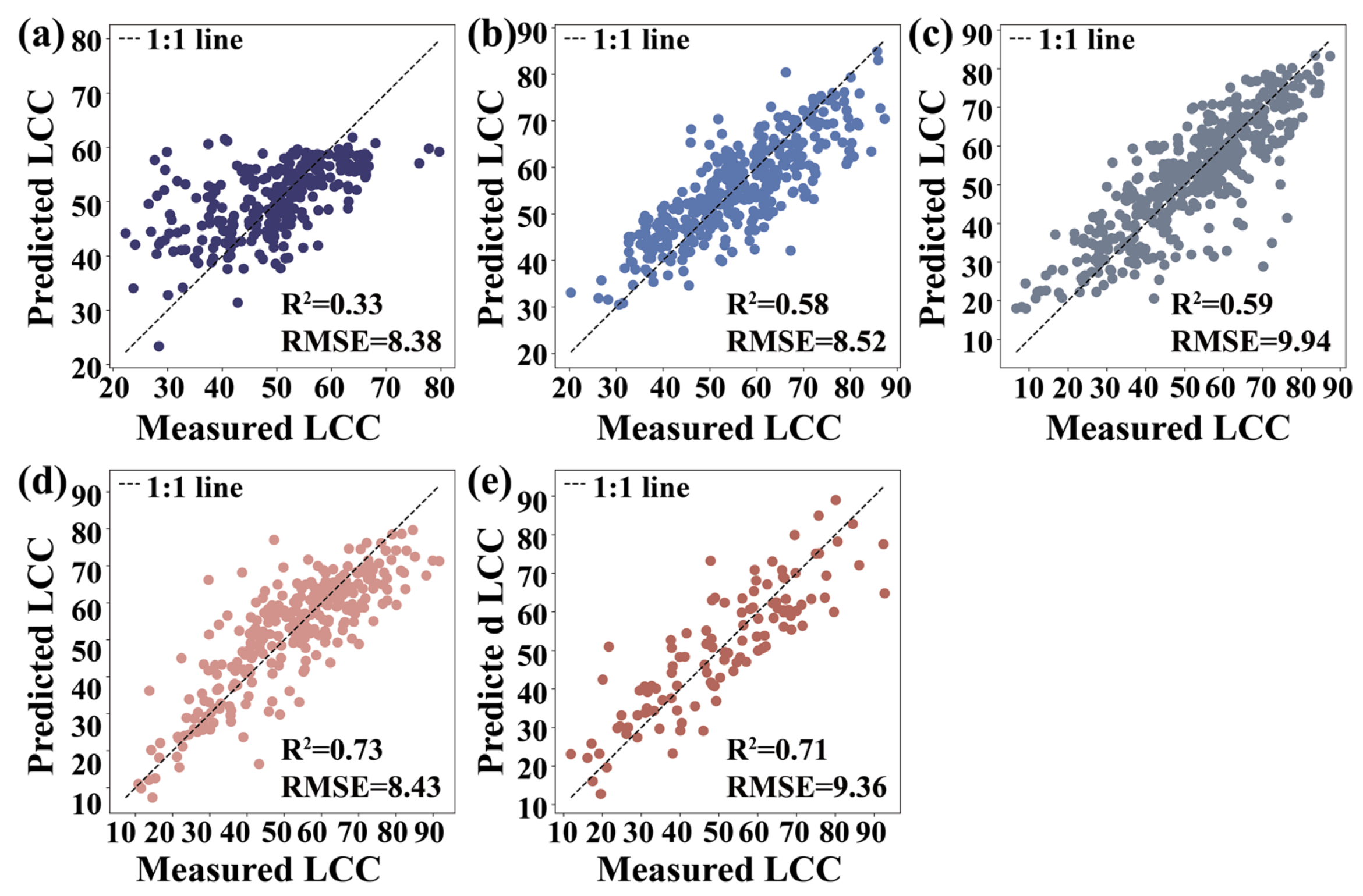
| Growth Seasons | RFR | KNNR | SVR | Parameters | |
|---|---|---|---|---|---|
| May | R2 | 0.42 | 0.34 | 0.33 | Carte4, FODS (647.2) |
| RMSE | 7.80 | 8.51 | 8.38 | ||
| June | R2 | 0.69 | 0.62 | 0.58 | VOG2, Carte4 |
| RMSE | 7.34 | 8.03 | 8.52 | ||
| August | R2 | 0.67 | 0.64 | 0.59 | VOG2, SR (750,710) |
| RMSE | 8.97 | 9.59 | 9.94 | ||
| October | R2 | 0.83 | 0.78 | 0.73 | VOG2, Carte4 |
| RMSE | 6.67 | 7.94 | 8.43 | ||
| December | R2 | 0.83 | 0.71 | 0.71 | FODS (730.2), (SDr − SDb)/(SDr + SDb) |
| RMSE | 7.13 | 9.18 | 9.36 |
Disclaimer/Publisher’s Note: The statements, opinions and data contained in all publications are solely those of the individual author(s) and contributor(s) and not of MDPI and/or the editor(s). MDPI and/or the editor(s) disclaim responsibility for any injury to people or property resulting from any ideas, methods, instructions or products referred to in the content. |
© 2023 by the authors. Licensee MDPI, Basel, Switzerland. This article is an open access article distributed under the terms and conditions of the Creative Commons Attribution (CC BY) license (https://creativecommons.org/licenses/by/4.0/).
Share and Cite
Li, D.; Hu, Q.; Ruan, S.; Liu, J.; Zhang, J.; Hu, C.; Liu, Y.; Dian, Y.; Zhou, J. Utilizing Hyperspectral Reflectance and Machine Learning Algorithms for Non-Destructive Estimation of Chlorophyll Content in Citrus Leaves. Remote Sens. 2023, 15, 4934. https://doi.org/10.3390/rs15204934
Li D, Hu Q, Ruan S, Liu J, Zhang J, Hu C, Liu Y, Dian Y, Zhou J. Utilizing Hyperspectral Reflectance and Machine Learning Algorithms for Non-Destructive Estimation of Chlorophyll Content in Citrus Leaves. Remote Sensing. 2023; 15(20):4934. https://doi.org/10.3390/rs15204934
Chicago/Turabian StyleLi, Dasui, Qingqing Hu, Siqi Ruan, Jun Liu, Jinzhi Zhang, Chungen Hu, Yongzhong Liu, Yuanyong Dian, and Jingjing Zhou. 2023. "Utilizing Hyperspectral Reflectance and Machine Learning Algorithms for Non-Destructive Estimation of Chlorophyll Content in Citrus Leaves" Remote Sensing 15, no. 20: 4934. https://doi.org/10.3390/rs15204934
APA StyleLi, D., Hu, Q., Ruan, S., Liu, J., Zhang, J., Hu, C., Liu, Y., Dian, Y., & Zhou, J. (2023). Utilizing Hyperspectral Reflectance and Machine Learning Algorithms for Non-Destructive Estimation of Chlorophyll Content in Citrus Leaves. Remote Sensing, 15(20), 4934. https://doi.org/10.3390/rs15204934