Abstract
Parcel-based crop classification using multi-temporal satellite optical images plays a vital role in precision agriculture. However, optical image sequences may be incomplete due to the occlusion of clouds and shadows. Thus, exploring inherent time-series features to identify crop types from incomplete optical image sequences is a significant challenge. This study developed a contrastive-learning-based framework for time-series feature representation to improve crop classification using incomplete Sentinel-2 image sequences. Central to this method was the combined use of inherent time-series feature representation and machine-learning-based classifications. First, preprocessed multi-temporal Sentinel-2 satellite images were overlaid onto precise farmland parcel maps to generate raw time-series spectral features (with missing values) for each parcel. Second, an enhanced contrastive learning model was established to map the raw time-series spectral features to their inherent feature representation (without missing values). Thirdly, eXtreme Gradient-Boosting-based and Long Short-Term Memory-based classifiers were applied to feature representation to produce crop classification maps. The proposed method is further discussed and validated through parcel-based time-series crop classifications in two study areas (one in Dijon of France and the other in Zhaosu of China) with multi-temporal Sentinel-2 images in comparison to the existing methods. The classification results, demonstrating significant improvements greater than 3% in overall accuracy and 0.04 in F1 scores over comparison methods, indicate the effectiveness of the proposed contrastive-learning-based time-series feature representation for parcel-based crop classification utilizing incomplete Sentinel-2 image sequences.
1. Introduction
Remote sensing techniques have long been an essential method for agricultural monitoring, with their ability to quickly and efficiently collect data on the spatial-temporal variability of farmlands and crops [1,2,3]. Remote sensing-based crop-type classifications could employ a small number of known samples to predict crop types for farmland fields. Thus, it is a crucial aspect of agricultural monitoring because it is fundamental for numerous precision agriculture applications (such as crop acreage and yield estimations) [4,5]. Due to the similarity of crop growth and the limited information from a single Earth observation, it can be challenging to distinguish between diverse crop types using a single satellite image, especially for crops grown during the same season. Exploring and learning time-series information from multi-temporal satellite images is, therefore, a promising method for improving crop classification [3,6,7,8]. Additionally, optical satellite images are easy to comprehend and interpret, as well as some vegetation indices (such as the normalized difference vegetation index, NDVI) derived from optical spectral bands, which can indicate crop growth stages explicitly. Traditionally, agricultural remote sensing applications have relied heavily on satellite data from optical sensors such as MODIS, Landsat, SPOT, and the Chinese Gaofen [5,9,10]. However, due to the occlusion of clouds and shadows, for a special location, optical image observation sequences may be incomplete, as some observations can be missing. This poses a significant challenge for these methods (especially in cloudy and rainy regions). On the one hand, the absence of images at essential phenological stages could lead to inadequate crop classification performance. On the other hand, incomplete image sequences increase difficulties when following tasks and severely restrict the application of time-series crop monitoring [11,12,13]. Therefore, how to extract inherent time-series features that can distinguish crop types from these incomplete observation sequences becomes the key to remote sensing and crop mapping [14,15].
Considerable research and effort have been devoted to constructing time-series features (representation) for improving crop classification [16], which can be categorized into three major groups, (1) important feature-based methods, (2) time-series composition methods, (3) time-series reconstruction methods, and others. Instead of reconstructing regular time-series images or features, important feature-based methods attempt to select prominent images captured during crucial phenological stages for crop identification [17]. For instance, rape and sunflower exhibit distinct yellow spectral features (with greater spectral reflectance on the red and green bands) during flowering, and paddy fields planted with rice seedlings are saturated with water, exhibiting higher water index values [3]. In other words, this method is based on an in-depth understanding of crop growth and phenology and attempts to identify crop types using minor but significant images. Some studies attempt to apply time-series filtering (such as S-G filtering) on incomplete multi-temporal images to manually generate phenological dates (such as the start or the end of the growing season) and then use these dates to identify crop types [18,19,20,21]. However, such methods rely heavily on satellite images during crucial phenological stages, which may not always be available. In addition, these methods can only differentiate between crops with significant phenological differences, such as winter wheat and summer corn. It is challenging to distinguish crops during the same seasons (for example, soy and corn).
Contrary to important feature-based methods, time-series composition methods attempt to use all available satellite images to construct more complete image sequences for crop classification (but with a longer time interval). In particular, the construction of satellite constellations significantly shortens their Earth observation (or revisit) periods. For instance, the revisit periods of the Sentinel-2 constellation with two satellites and the virtual constellation between Landsat-8 and Landsat-9 are five and eight days, respectively. Multiple images are captured by these satellites during a particular phenological stage. Therefore, these images with close acquisition dates can be composited and mosaiced to produce composited images with lower cloud/shadow coverage [22]. Such approaches can significantly enhance the completeness of time-series observations. However, such methods expand the spectral ranges of crop phenological stages, resulting in mixed feature spaces and overlapping type spaces for crop mapping [23]. Meanwhile, this kind of method has limited improvement in crop classification. In addition, they cannot completely eliminate the missing values to construct regular time-series observations in cloudy and rainy regions.
Time-series reconstruction methods are promising alternatives for dealing with incomplete time-series observations. By exploring spatial similarity, spectral correlation, and temporal trends, time-series reconstruction can predict cloud- and shadow-covered pixels to generate regular time-series images [12,13]. Compared to time-series composition methods, these methods produce time-series images with original (or even shorter) time intervals, which are practical and effective in time-series crop classification. Nevertheless, a few studies [12,24] found that a larger percentage of missing data (including significant gaps in timestamps and large-area missing) results in greater uncertainty and over-smoothing, which could mislead subsequent time-series analysis. In addition, time-series reconstruction methods necessitate additional effort.
To address the issue of incomplete time-series data, another idea is to design algorithms that are capable of utilizing incomplete time series directly. Recent developments in machine learning have also begun to address the issue of an incomplete time-series analysis. For instance, by default, the eXtreme Gradient-Boosting (XGBoost) algorithm can handle missing values. Whenever a missing value is encountered during XGBoost-based prediction, a default (right) direction is created at each tree node [25,26]. In addition, masking layers can be used to identify the missing position in time-series data and then feed them directly into Long Short-Term Memory (LSTM)-based networks.
Despite this encouraging improvement in time-series feature representation for crop classification using incomplete image sequences achieved using the aforementioned methods, these approaches have a number of limitations: (1) Existing techniques have not established a general framework for constructing or learning inherent time-series feature representations from incomplete image sequences. Moreover, manually crafted features are limited in their ability to identify specific crop types or phenological periods. (2) Supervised LSTM-based methods typically require a large number of labeled samples for training. It is, thus, difficult to directly apply them in remote sensing applications with limitations in labeling [3]. (3) From the standpoint of implementation, algorithms like XGBoost use a default or assumed trick to handle missing values in time-series data, as opposed to producing regular feature representation. Therefore, can a general framework be developed to represent inherent time-series features from incomplete image sequences in crop classification?
Recent research has focused more on self-supervised learning to extract effective representations from unlabeled data. Self-supervised pre-trained models with limited labeled data can achieve comparable performance to supervised models trained on complete and labeled data. Particularly, contrastive learning has recently demonstrated its strength for self-supervised representation learning in the computer vision domain due to its capacity to learn invariant representations from augmented data [27,28]. Contrastive learning explores numerous views of input images through the utilization of data augmentation techniques. It subsequently learns inherent representations by maximizing the similarity between views originating from the same sample while minimizing the similarity between views from distinct samples. This technique is widely employed in healthcare data analysis, visual comprehension, and natural language processing [24,29,30], but it has been underexplored for remote sensing time-series analysis [31].
This research aims to develop a general framework for inherent time-series feature representation from incomplete satellite image sequences to improve crop classification. This method was implemented by combining contrastive-learning-based feature representation with machine-learning-based classifications. Compared to previous approaches, this study combines three principal contributions. The first contribution involves a contrastive-learning-based framework for time-series feature representation from incomplete satellite image sequences. The second is developing a type-wise consistency augmentation and type-wise contrastive loss to enhance contrastive learning for supervised time-series classification. The third is an in-depth analysis of the effect of contrastive-learning-based feature representation. The proposed method is further discussed and validated through parcel-based time-series crop classifications in two study areas (one in Dijon of France and the other in Zhaosu of China) with Sentinel-2 image sequences in comparison to existing methods.
2. Study Area and Datasets
2.1. The Dijon Study Area
The first study area is Dijon, located in the Côte-d’Or department (with the Dijon prefecture) in the Bourgogne-Franche-Comté region of northeastern France at 05°01′E and 47°17′N in geographical coordinates (latitude/longitude) on the WGS-84 ellipsoid (Figure 1). The study area, covering a total area of approximately 5000 km2, features an oceanic climate with a continental influence under the Köppen climate classification, with average temperatures between 6.8 °C and 16.1 °C and an annual average precipitation level of 740 mm. These climatic conditions are ideal for growing wheat, rape, grape, and grass.
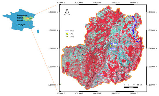
Figure 1.
The Dijon study area is in the northeast of France. The right-hand section provides an overview of the near-infrared-blue-green Sentinel-2 image acquired on the day of the year (DOY) 263 in 2019.
Under the Common Agricultural Policy of the European Union, the National Institute of Forest and Geography Information (IGN) of France is responsible for gathering geographical information on the geometry of cultivated crops. The IGN institute has released anonymized parcel geometries and types of cultivated crops under an open license policy. This study used data collected in 2019 to validate the proposed model. In the raw crop type categories, there were 328 distinct crop labels organized into 23 groups. ‘Winter wheat’ (WWT), ‘winter barley’ (WBR), ‘winter rapeseed’ (WRP), ‘winter triticale’ (WTT), ‘spring barley’ (SBR), ‘corn’ (CON), ‘soy’ (SOY), ‘sunflower’ (SFL), ‘grape’ (GRA), ‘alfalfa’ (AFF), ‘grass’ (GRS), and ‘fallow’ (FLW) were selected and summarized for the Dijon study area. The two minority classes (‘sunflower’ and ‘winter triticale’) were also retained to challenge classification methods. This further reflects the significant class imbalance in real-world crop-type-mapping datasets [32]. This study area encompassed approximately 53,400 parcels, of which 20% were selected randomly to serve as labeled samples.
In addition, Sentinel-2 time-series images (with a Path/Row of T32TFN) captured between February 2019 and September 2019 were used to record crop growth, as the growth stages of winter crops are also concentrated in the subsequent year. The Sentinel-2 satellite image contained four (visible and near-infrared) bands with a spatial resolution of 10 m and six (red edge and shortwave infrared) bands at a 20 m resolution. All 48 images, captured every 5 days, were obtained from the Copernicus Open Access Hub at Level 1C, and 38 of them contained cloud and shadow contamination. Meanwhile, images captured on the days of the year (DOY) 48, 58, 88, 133, 143, 168, 178, 233, 238, 258, and 263 were free from clouds and shadows.
2.2. The Zhaosu Study Area
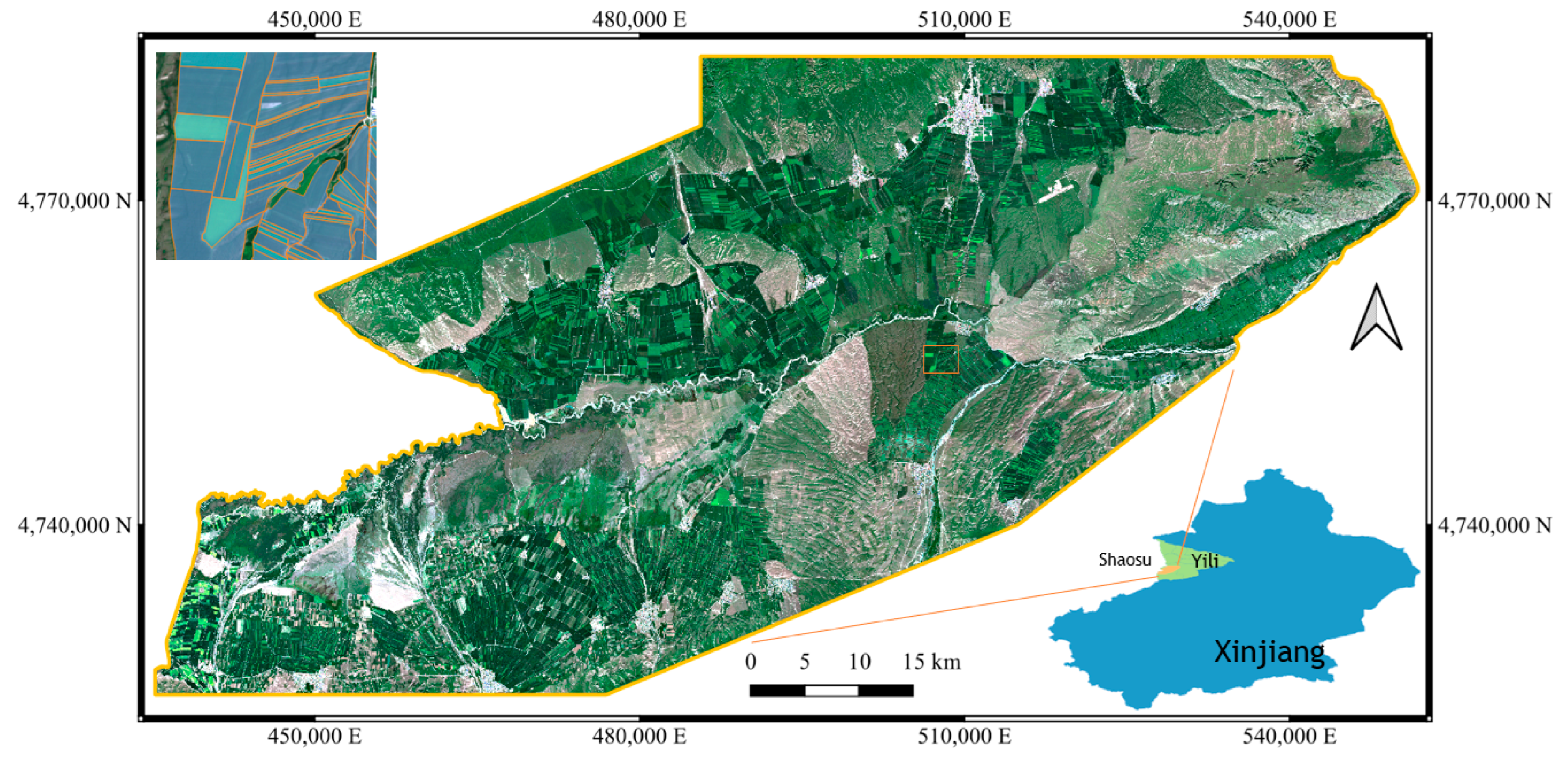
The second study area is Zhaosu, situated southwest of Yining City, Xinjiang Autonomous Region, China (latitude range: 43°09′N to 43°15′N and longitude range: 80°08′E to 81°30′E in geographical coordinates) (Figure 2). It is a highland basin surrounded by mountains in the Central Asian hinterland, with an elevation ranging from 1323 m to 6995 m. It is dominated by a continental temperate semi-arid semi-humid cool climate, with an annual average temperature of 2.9 °C and 512 mm of annual precipitation. The majority of Zhaosu is covered by calcium-rich black soil with a thick humus layer and a high organic matter content. These natural geographical and climatic conditions are optimal for the growth of spring rapeseed (from April to September), making Zhaosu the largest producer of spring rapeseed in Xinjiang.
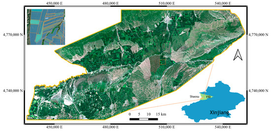
Figure 2.
The Zhaosu study area is located in Xinjiang’s northwestern region. The center section provides an overview of the Sentinel-2 image acquired on the DOY 190 in 2020 (with the true-color composition). The top left corner presents local details of parcel geometry.
Official farmland parcel maps are unavailable for this study. Consequently, Chinese Gaofen-1 (GF-1) satellite images were used to delineate the precise geometries of farmland parcels. The GF-1 images included one panchromatic band with a 2 m spatial resolution and four multi-spectral bands (blue, green, red, and near-infrared) with an 8 m spatial resolution. Using the Gram–Schmidt spectral sharpening algorithm, the panchromatic and multi-spectral bands were combined to produce a multi-spectral pan-sharpened image with a 2 m spatial resolution. Two GF-1 images acquired in July 2020 with 60 km-wide swaths were registered and mosaicked to cover the study area. In this study, approximately 11,400 parcels were obtained.
In July 2020, field surveys for supervised crop classification and accuracy assessments were conducted. To facilitate the field surveys, sample sites were distributed along the roads. In surveys, a handheld GPS device (with a precise point positioning precision level of 3.0 m) was utilized to record geographic location (in the WGS84 geographic coordinate system). Approximately 1000 parcel samples were collected (200 rapeseed parcels and 800 parcels with other crops, proportional to the percentage of rapeseed-planted area). Therefore, this study designed a binary classification schema containing rapeseed and other types.
Two Sentinel-2 images (with P/R of T44TMN and T44TNN) captured on the same day were mosaiced to cover the Zhaosu study area. And 36 observations between April and September 2020 were used to identify rapeseed. Also, images acquired on DOY 115, 145, 165, 185, 190, 195, 220, 235, 255, 260, and 265 in 2020 were totally clean.
The datasets and crop growth periods are summarized in Table 1. The two study areas were distinguished by distinct climatic and topographical conditions. In addition, the cultivation status of crops varied considerably based on crop type and farming technique. These circumstances were sufficient for validating the proposed model.

Table 1.
Datasets and crop growth periods in the Dijon and Zhaosu study areas.
3. Methodology
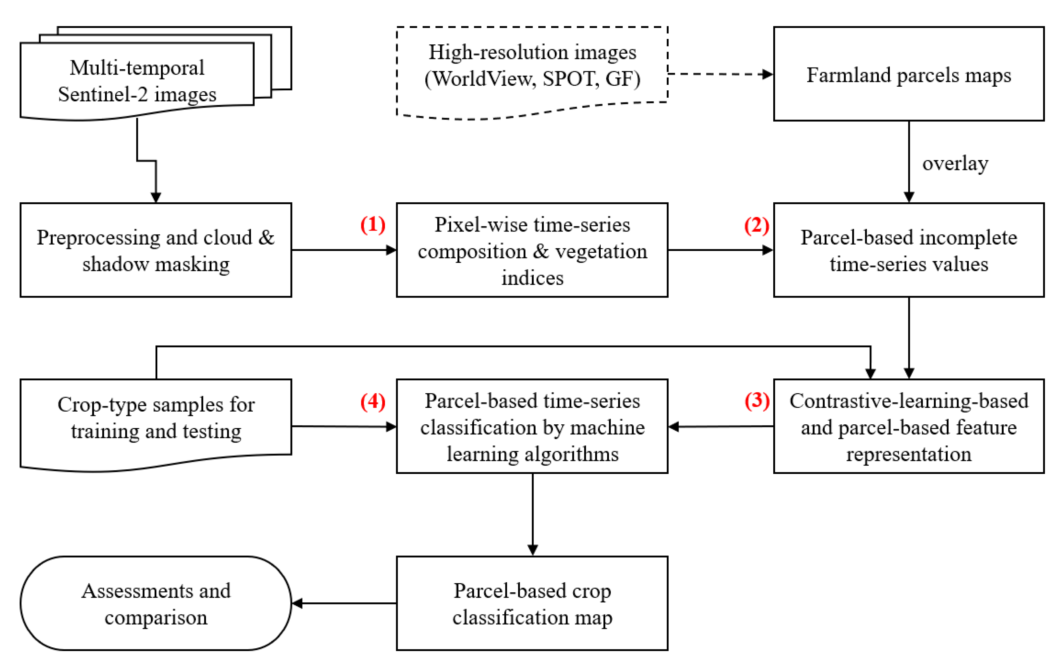
Time-series feature representations using contrastive learning were employed to improve parcel-based crop mapping using multi-temporal Sentinel-2 images, as illustrated in Figure 3. This procedure consisted of four major steps: (1) pixel-wise spectral features, (2) parcel-based spectral features, (3) time-series feature representation, and (4) time-series crop classification.
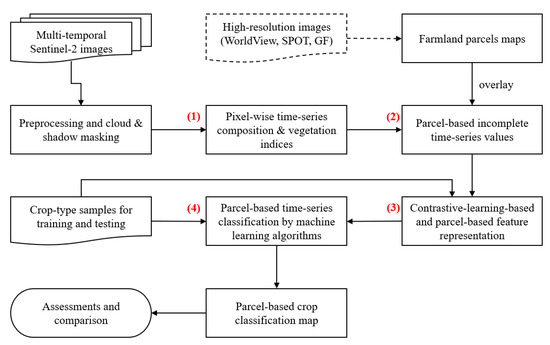
Figure 3.
Flowchart of contrastive-learning-based time-series feature representation for parcel-based crop classification.
Before the main process, data preprocessing was performed, including atmosphere calibration, the cloud/shadow-based masking of Sentinel-2 images, the geographic registration of experimental data (including Sentinel-2 images, farmland parcel maps, and survey samples), and the generation of farmland parcel maps. First, at the pixel scale, time-series composition and band calculation were applied to Sentinel-2 images to generate spectral features and vegetation indices. Second, cloud/shadow-masked Sentinel-2 feature images (including spectral bands and indices) were overlaid onto parcel maps to generate parcel-based incomplete time-series spectral features (with missing values). Third, at the parcel scale, a contrastive learning framework was enhanced to map time-series spectral features into their inherent feature representation (without missing values). Finally, using the feature representation and time-series classifiers, parcel-based crop classification maps were generated.
3.1. Data Preprocessing
3.1.1. Farmland Parcel Maps
Parcel-based crop mapping requires known farmland parcel geometries that are accessible in most regions of Europe [32] (including the Dijon study area). In the absence of geometry data (as in the Zhaosu study area), farmland parcel maps were generated from high-spatial-resolution images (the GF-1 images used for Zhaosu) using the method detailed in our previous study [33]. First, roads, waterlines, and terrain lines derived from DEMs were used to spatially split the GF-1 images of study areas into multiple subareas. Then, in each subarea, the trained (by manually labeled samples of parcel boundaries) boundary-semantic-fusion convolutional neural network (BSNet) [33] was utilized to automatically generate binary raster maps of parcel boundaries. Finally, automatic postprocessing (including the vectorization of binary parcel boundaries, topology checks on parcel geometries, and the removal of small polygons) and the manual correction of parcel polygons were applied to generate precise farmland parcel maps.
3.1.2. Sentinel-2 Images
On Sentinel-2 L1C images, the Sen2Cor algorithm was first applied for atmosphere calibration to generate bottom-of-atmosphere data where images acquired over time and space shared the same reflectance scale, thereby enhancing crop mapping when monitoring large-scale areas over time [34]. Four spectral bands (bands 2, 3, 4, and 8) with a spatial resolution of 10 m and six spectral bands (bands 5, 6, 8A, 11, and 12) with a spatial resolution of 20 m were produced for each Sentinel-2 image.
A quality scene classification (SLC) band, which labels pixels obscured by clouds and shadows, was created using the Sen2Cor algorithm in the meantime. Misclassification in the SLC band was further corrected through expert visual interpretation, particularly at the cloud and shadow edges. Then, the SLC band was reclassified into a binary classification to generate a final masking band, one indicating clean pixels and the other for contaminated pixels (including cloudy and shadowy regions and no data value regions). Finally, masked images were generated by overlaying the masking band on Sentinel-2 images and setting the spectral reflectance values of pixels in masked regions to a default masking value (0 in our experiments).
3.2. Pixel-Wise Spectral Features
3.2.1. Time-Series Composition
Multi-temporal value composition is a common technique for suppressing atmospheric and cloud effects and reconstructing time-series observations when processing time-series optical images [35]. This technology was employed to generate time-series images with lower cloud and shadow contamination. It was also noted that time-series composition could increase observation intervals, resulting in sparser time-series sequences.
Greater vegetation index values indicated a much more robust vegetation growth. Alternatively, this assumption may not hold true for spectral reflection. For instance, cloudy pixels with higher spectral values and shadowy pixels with lower values are contaminated. Consequently, a mean value composition algorithm was utilized in this study. Following a similar procedure of maximum value composition, mean value composition was applied to multi-temporal Sentinel-2 images to generate a composited image using the following equation.
where N(i,j) is the number of clean observations (not covered by clouds and shadows) at a geographical location (i,j), v(i,j)t is the pixel-wise spectral value of time step t at location (i,j) and mvc(i,j) is the composited value at location (i,j).
3.2.2. Vegetation Indices
Typically, the vegetation index is derived from optical red and near-infrared (NIR) reflectance via linear or non-linear combination operations. They are simple but effective parameters for characterizing vegetation cover and growth status in agricultural remote sensing applications. Additionally, compared to other multi-spectral images (such as Landsat images), Sentinel-2 images contain three additional red-edge bands that are sensitive to vegetation growth [36]. To expand spectral features for Sentinel-2 images, eight vegetation indices, including NDVI, EVI, MTCI (terrestrial chlorophyll index), NDRE (normalized difference red edge index), MCARI2 modified chlorophyll absorption ratio index), REP (red edge position), IRECI (novel inverted red-edge chlorophyll index), and CIred-edge (red-edge chlorophyll index) were calculated [37,38]. Also, to maintain an exact spatial resolution of 10 m, the 20 m spectral bands were resampled into 10 m using the nearest neighbor sampling algorithm when calculating vegetation indices.
3.3. Parcel-Based Time-Series Features
Multi-temporal processed Sentinel-2 images (including spectral bands and derived vegetation indices) were overlaid onto parcel maps of farmland to generate parcel-based time series. Spectral values were averaged over the bounds of parcel geometry. In Sentinel-2 bands, pixels within a parcel polygon were first searched. Then, the average spectral value of these pixels was taken as the feature value of this parcel. When parcels were entirely covered by clouds and shadows, their features were assigned the default masking value of 0. When parcels were partially covered, the spectral values of clean pixels were averaged. Finally, for each parcel, a feature vector was generated, where D is the number of spectral bands, and T is the number of satellite observations.
3.4. Time-Series Feature Representation
This study employed contrastive learning to transform spectral features into time-series feature representations. There are three advantages to this. First, feature representation contributes to learning the inherent time-series feature for classification. Second, it can generate complete and regular time-series features (without missing values). Thirdly, it can decrease the demand for a larger number of labeled samples in deep-learning-based applications. A general framework (known as TS2Vec) was proposed for learning the representation of time series [39]. It consists of three main components: a representation framework, consistency augmentation, and loss functions. Feature representation was performed using the representation framework. Using consistency augmentation, augmented sample pairs were generated to train the framework. Loss functions ensured the discovery of consistent features from multiple augmented samples.
This study attempted to improve the TS2Vec model for supervised time-series crop classifications (named type-wise TS2Vec) by incorporating prior-type information from labeled samples into contrastive learning. In general, we followed the architecture of the TS2Vec model [39]. Further, the consistency augmentation and contrastive loss were enhanced. (1) When conducting consistency augmentation, we discarded original random cropping and developed novel type-wise random selection and random band-masking techniques. (2) When calculating multi-scale contrastive loss, type-wise contrastive loss was devised to replace instance-wise loss.
3.4.1. Consistency Augmentation
The establishment of positive sample pairs is fundamental in contrastive learning. Various augmentation strategies for general time-series tasks have been proposed in previous studies [39,40,41]. For supervised time-series crop classification tasks, it is essential to ensure the following characteristics: (1) preserving the magnitude of time-series values, (2) retaining the length and timestamp of the time series when exploring phenological characteristics of crop growth, (3) exploring correlations between bands given that these correlations are higher; and (4) introducing crop-type information to enhance consistency augmentation.
Based on these assumptions, the random cropping technique in the TS2Vec model was eliminated due to its inconsistency with the assumption (2). Then, inspired by assumptions (3), and (4) a random band masking technique and a type-wise random selection technique were implemented, respectively. Incorporating the random timestamp masking proposed by [39], we generated consistency augmentation, in which feature representations at the same timestamp in two augmented contexts with the same crop types were considered positive pairs.
- Type-wise random selection
Available type labels are high-quality-supervised information for constructing augmented contexts in contrastive learning for time-series crop classification. As shown in Figure 4, this study proposed a type-wise random selection algorithm to construct augmented contexts in batch training.
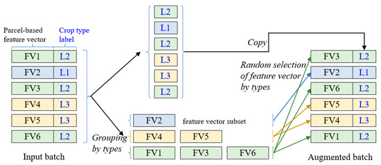
Figure 4.
Type-wise random selection to construct augmented contexts in batch training. Background colors indicate different crop types.
A sample consists of a parcel-based feature vector and a crop-type label. First, in a sample batch, crop type labels (L) of each instance sample were recorded in order, and feature vectors (FV) of instance samples with the same type labels were compiled into a subset. Then, the recorded crop-type labels were replicated as augmented crop-type labels. In addition, for each crop-type label, a feature vector (FV) was randomly selected from the feature vector subset with the same crop-type labels as the augmented feature vectors. Finally, the selected feature vector was combined with the crop-type label to produce a type-wise augmented sample. Multiple instances of the same crop type labels are required for type-wise random sampling. Therefore, a batch size greater than the total number of crop-type labels was set.
- Spectral band masking
Spectral band masking can also be adapted to generate new contexts. For each time-series input, one spectral band was randomly selected and masked (setting their values to 0) to generate an augmented context view. Furthermore, in two context reviews, their contextual representations should be consistent. The contrastive learning framework could capture band-to-band correlations through spectral band random masking to establish inherent feature spaces for crop classification.
3.4.2. Type-Wise Contrastive Loss
Multi-scale contrastive loss was employed to force the encoder to learn feature representations at multiple scales [39]. At each scale, the TS2Vec model jointly leverages both instance-wise and temporal contrastive losses to capture a contextual representation of time series. In the instance-wise loss, representations of other instances at timestamp t were taken as negative samples to capture fine-grained representations for general time-series tasks. For time-series classification tasks, this restriction was too strict for different instances with the same class types (categories). Thus, we attempted to utilize a supervised type of information for labeled samples to lift this restriction by taking representations with the same class type c and at timestamp t as positive samples. The type-wise contrastive loss indexed with (i, t) can be formulated as follows:
where i is the index of the input sample, B denotes the batch size, and and denote representations for the same timestamp t and from two augmentations of one sample.
3.5. Time-Series Classification
Based on the time-series feature representation, a traditional machine-learning-based (XGBoost-based) classifier and an LSTM-based classifier were applied to generate crop classification maps.
3.5.1. XGBoost-Based Classifier
XGBoost is a highly efficient and widely used implementation of the gradient-boosted trees algorithm [25]. It is a supervised learning algorithm for regression, classification, and ranking problems, which uses sequentially built shallow decision trees to provide accurate results. In this study, the XGBoost algorithm with a “gbtree” booster and a “softmax” objective was utilized to build XGBoost-based classifiers. In addition, the GridSearchCV technique was used to conduct hyperparameter tuning to determine the optimal parameter values for crop classification.
3.5.2. LSTM-Based Classifier
In recent years, the recurrent neural network (RNN) and its variants (such as LSTM) have been utilized extensively in time-series analysis, such as time-series prediction [12,13] and time-series classification [3,8]. This study employed stacked LSTM models for crop classification [3]. In LSTM-based classification models, four LSTM layers with h (where h equals the dimension of input features) hidden neurons were first stacked to transform input time-series features into high-level features. Then, a dense layer fully connected high-level features to crop categories. A SoftMax activation function then outputs crop-type probabilities to generate crop classification maps. Furthermore, a cross-entropy loss function and an Adam (Adaptive Moment Estimation) optimizer with default parameters were employed to train LSTM-based classifiers.
3.6. Performance Evaluation and Comparison
3.6.1. Comparative Methods
To validate the effectiveness of contrastive-learning-based feature representation, several classification comparisons utilizing different time-series feature representations were performed. The baseline classification is an XGBoost-based classifier only using completely Clean Sentinel-2 images (referred to as XGB-Clean). Using all available Sentinel-2 time-series (TS) images, an LSTM-based time-series classifier and an XGBoost-based time-series classifier (referred to as LSTM-TS and XGB-TS, respectively) were constructed. Using time-series Feature Representation (FR) generated from the proposed contrastive learning framework, an LSTM-based classifier and an XGBoost-based classifier (referred to as LSTM-FR and XGB-FR, respectively) were also built. In addition, GridSearchCV was used to conduct hyperparameter tuning for the XGB-Clean, XGB-TS, and XGB-FR classifiers.
For classifiers, sample sets were randomly divided into training, validation, and testing sets in a ratio of 6:2:2, for both the proposed type-wise TS2Vec model and time-series classifiers.
3.6.2. Evaluation Metrics
Based on the confusion matrix [42], which was created by comparing classification results to test samples parcel by parcel, overall accuracy (OA), precision (P), recall (R), and F1 scores were extracted to evaluate crop classification accuracy. The OA was determined by dividing all correctly classified parcels by the whole validation dataset. Precision and recall were calculated using Precision = TP/(TP + FP), Recall = TP/(TP + FN), where TP, TN, FP, FN represent the number of true positive, true negative, false positive, and false negative parcels, respectively, in the confusion matrix. In addition, F1 = 2 × UA × PA/(UA + PA), the harmonic mean of the PA and UA, was more meaningful than OA for a special crop type. Greater OA, P, R, and F1 scores indicated superior results, and vice versa.
4. Results and Discussion
4.1. Results
4.1.1. Results in Dijon
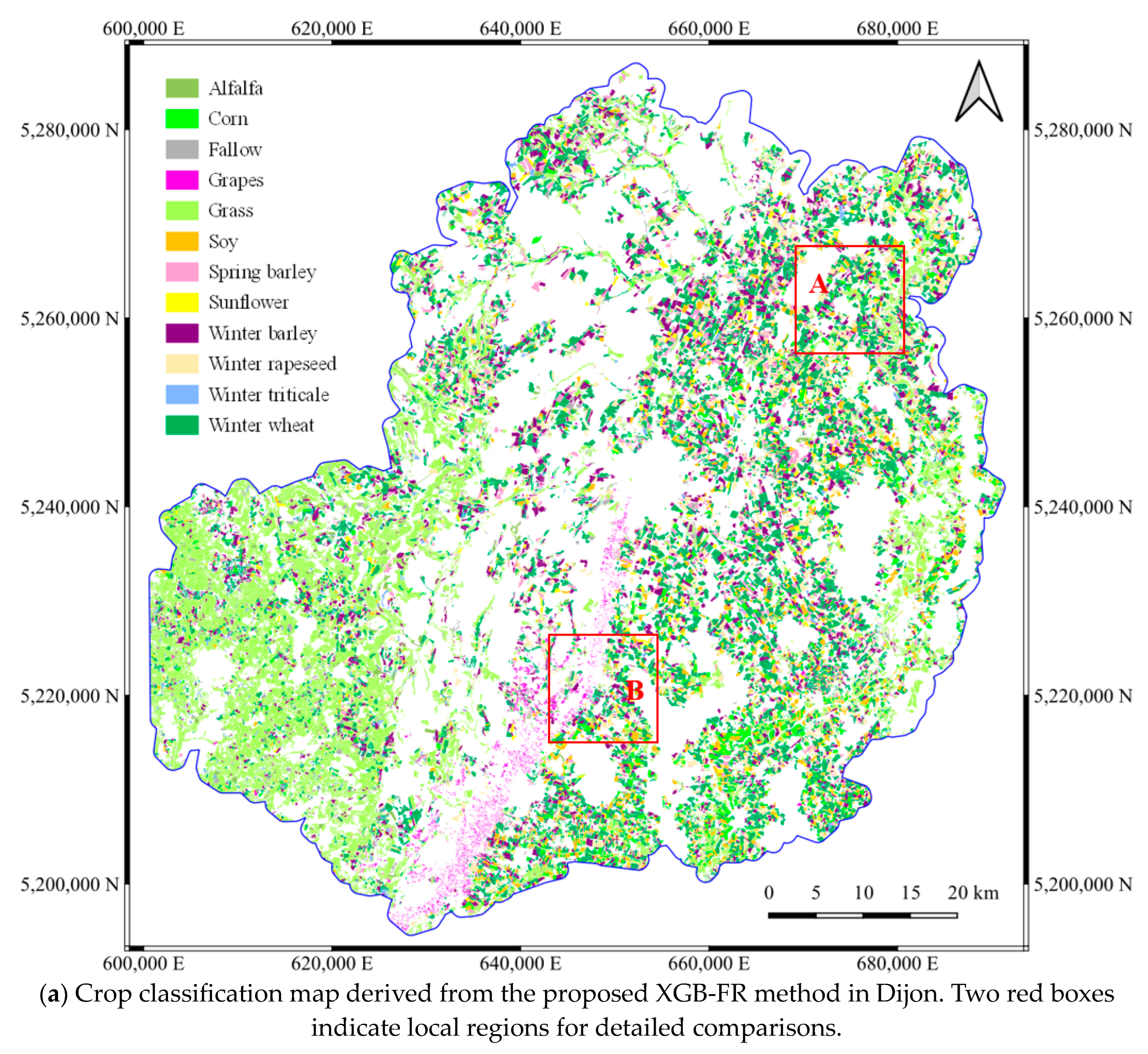
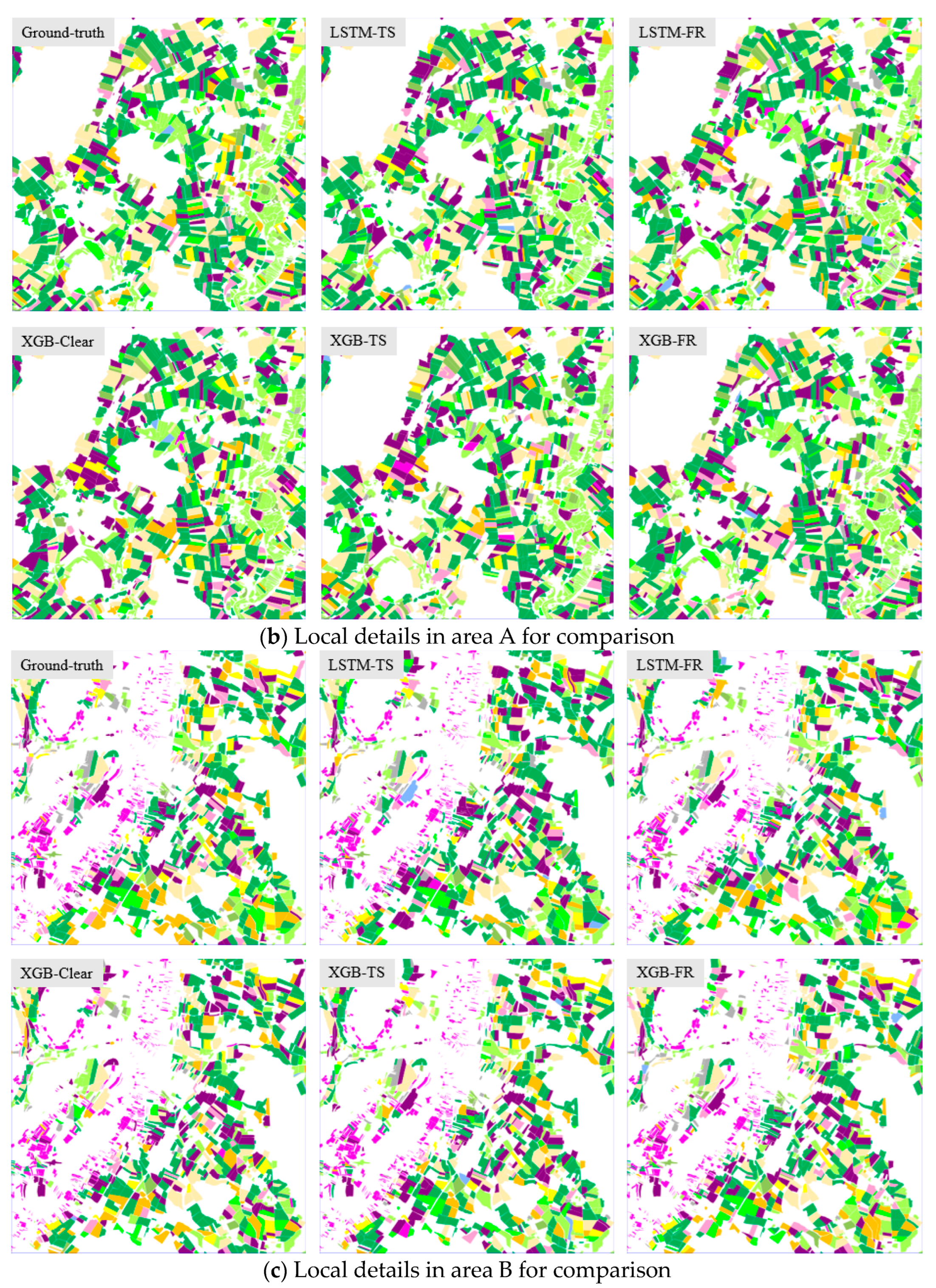
Crop classification maps and local details generated using the proposed XGB-FR method and comparison approaches are presented in Figure 5. Limits to the manual interpretation of multi-temporal images make it difficult to evaluate classification performance through visual interpretations qualitatively. Nonetheless, overall performance can be evaluated in local regions. ‘Grass’ is mainly distributed along the riverbanks of the Vingeanne (local region A in Figure 5) and to the southwest of the study area (Figure 5). ‘Grape’ is mainly cultivated in the narrow valley from Chenôve to Beaune (local region B in Figure 5). The flatlands in the east-central region were covered by ‘winter wheat’, ‘winter barley’, ‘corn’, and so on.
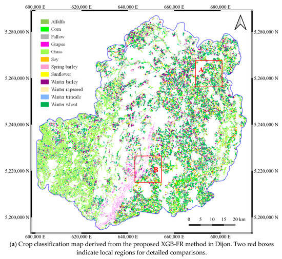
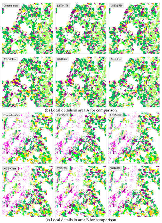
Figure 5.
Results of parcel-based crop mapping using comparative methods in the Dijon study area. (a) presents the whole crop classification using the XGB-FR method, (b,c) present the local details of crop classification from five comparison methods.
Table 2 provides a summary of the classification accuracies (OA, Precision, Recall, and F1 for the Dijon study area) generated from five comparison approaches.

Table 2.
Comparison of classification accuracies in the Dijon study area (underline indicates the best scores).
Overall, XGB-FR and LSTM-FR classifications employing feature representation performed significantly better than other classifications, with OA scores above 83.00%, precision scores exceeding 72.00%, recall scores exceeding 77.00%, and F1 scores exceeding 0.74, respectively. The XGB-TS and LSTM-TS classifications using raw time-series spectral features were followed, with OA scores of about 80.00%, precision scores of approximately 64.00%, recall scores of approximately 74.00%, and F1 scores of approximately 0.68, respectively. This indicates that the proposed contrastive learning framework could explore the inherent time-series features of crop growth to increase classification accuracy. With an OA of 76.92%, a precision of 56.14%, a recall of 65.93%, and an F1 score of 0.61, the XGB-Clean classification utilizing only clean images produced the worst results. This was expected given that these clean images are time-series spare. It is difficult to capture the essential phenological characteristics for classification, especially in July when crops grow rapidly.
The LSTM-TS classification performed marginally better than the XGB-TS classification when employing raw time-series spectral data. The possible reasons behind this are that LSTM models capture the long- and short-term dependence in the raw time-series observation, which is essential for crop identification. While using time-series feature representation, the XGB-FR classification surpassed the LSTM-FR classification. On the one hand, the proposed contrastive learning framework can explore the multi-scale dependencies from raw spectral features and express them in generated feature representation. On the other hand, XGBoost classifiers applied boost tree rules to feature representation and improve crop classification further. In other words, the best crop classification was made possible by the combined advantages of contrastive-learning-based representation and XGBoost-based classifiers.
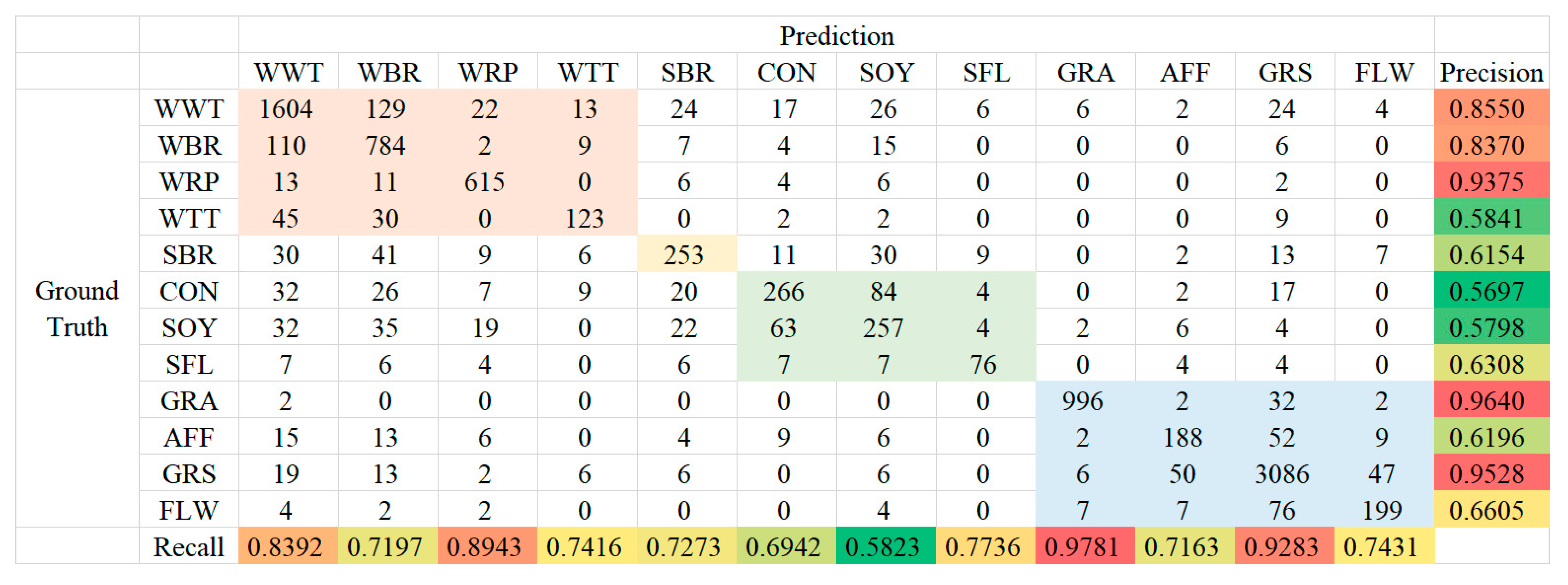
To analyze the benefit of feature representation, the confusion matrix (normalized with range [0, 10,000]) retrieved from the XGB-FR classification is presented in Figure 6.
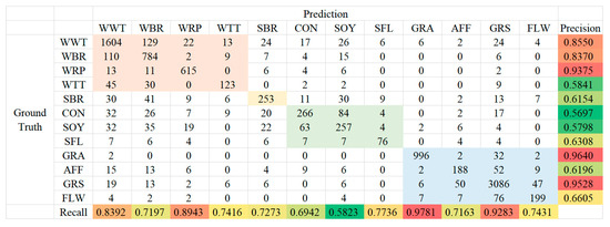
Figure 6.
Confusion matrix for the XGB-FR classification. Light orange, light yellow, light green, and light blue indicate winter crops, spring crops, summer crops, and other crops, respectively.
‘Winter rape’, ‘grape’, and ‘grass’ achieved precision scores greater than 0.90, followed by ‘winter wheat’ and ‘winter barley’ with precision scores greater than 0.80. With precision scores less than 0.60, ‘winter triticale’, ‘corn’, and ‘soy’ obtained the worst results. This relates to the a priori distribution of crops in the study area. To improve overall accuracy, statistical classifiers tend to classify samples into larger categories when these categories are unbalanced. In addition, ‘grass’ and ‘grape’ achieved the highest precision and recall scores.
When examining the confusion matrix in detail, it was found that it could be divided into a number of sub-regions (as depicted in different colors in Figure 6), including winter crops (‘winter wheat’, ‘winter barley’, ‘winter rape’, and ‘winter triticale’, indicated by light orange color), summer crops (‘corn’, ‘soy’, and ‘sunflower’, indicated by light green color), spring crop (‘spring barley’ indicated by light yellow color), and other crops (indicated by light blue color). On the one hand, heterogeneity between subregions is relatively high. For example, the planting, growth, and harvesting schedules for autumn crops are entirely distinct from those of summer crops. Thus, they are less likely to be misclassified relative to one another. By contrast, there are numerous misclassifications within this subregion due to their similar phenology (such as pairs of ‘corn’ and ‘soy’, ‘wheat’ and ‘barley’, ‘grass’ and ‘alfalfa’). In addition, it was found that ‘winter rapeseed’ has a higher precision score in the winter-crop sub-region. Its unique yellow flowers contribute to this.
4.1.2. Results in Zhaosu
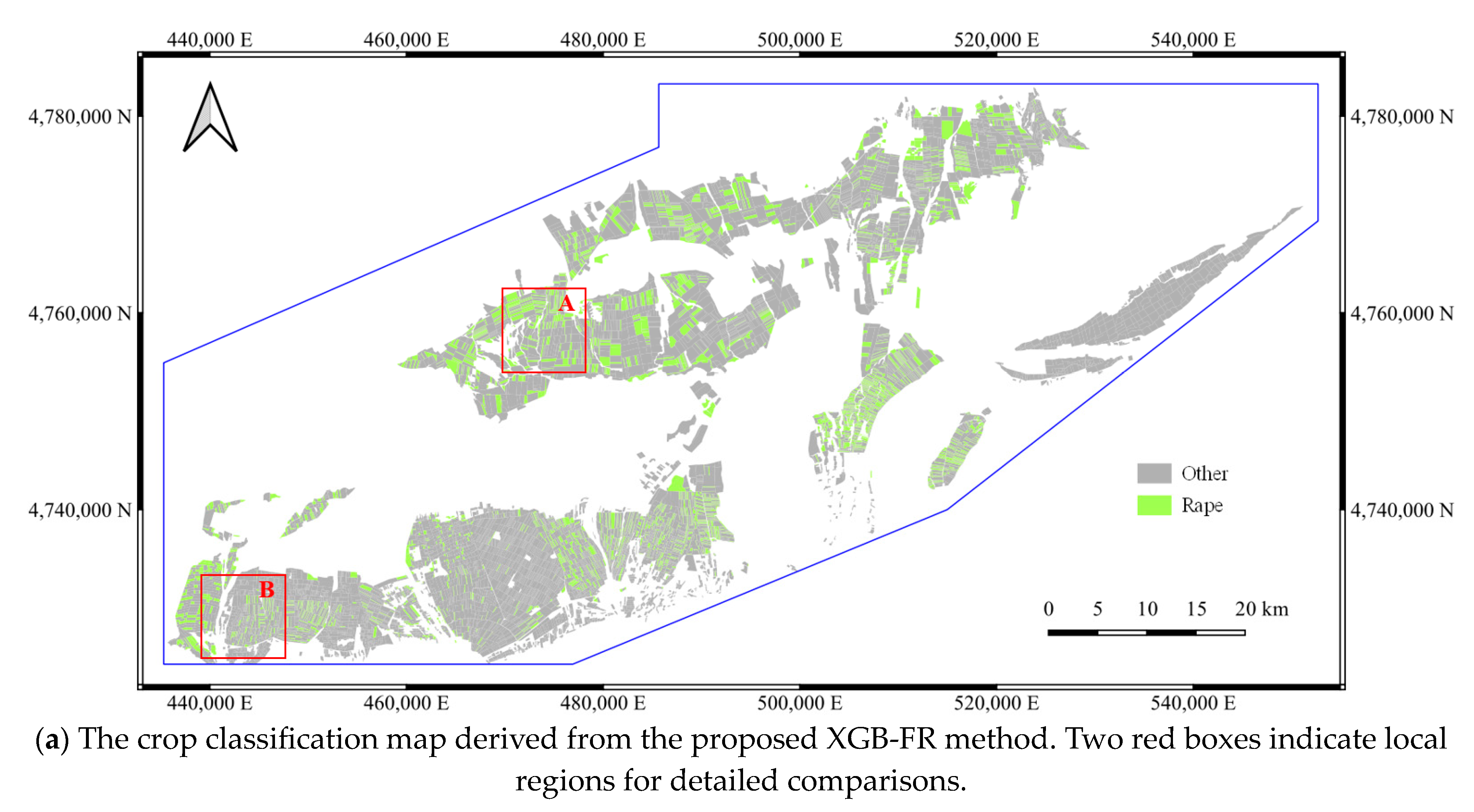
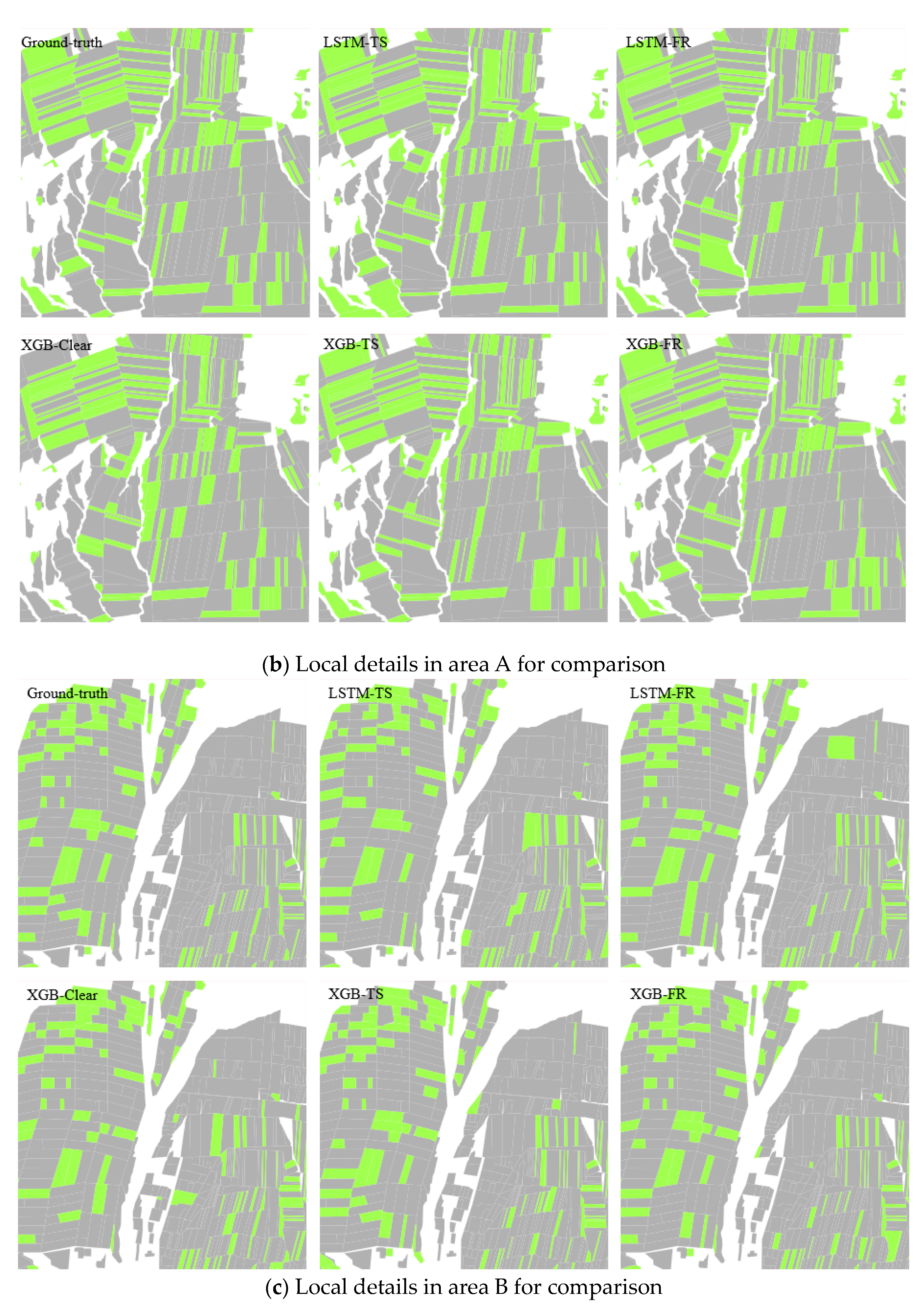
The crop classification map resulting from the proposed method and local comparative details from the five methods are displayed in Figure 7. In general, ‘spring rapeseed’ was widely distributed in the study area, with the exception of the eastern river valley. ‘Spring rapeseed’ was planted on larger parcels in the western and northern regions and on tiny parcels in the southern region where residents reside.
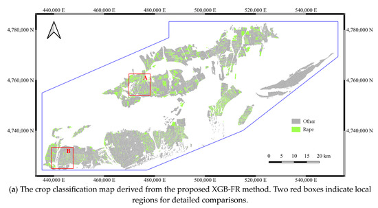
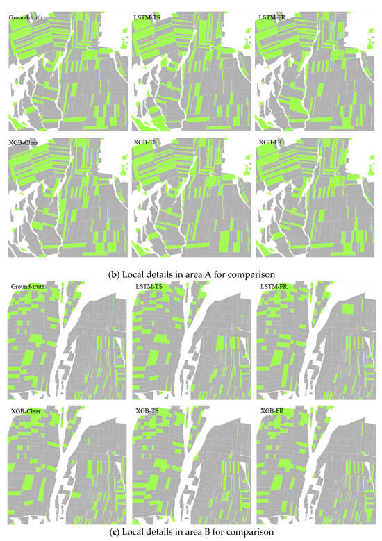
Figure 7.
Results of parcel-based crop mapping in the Zhaosu study area. (a) presents the whole crop classification using XGB-FR method, (b) and (c) present the local details of crop classification from five comparison methods.
Also, the classification accuracies derived from the five comparative methods were summarized, as illustrated in Table 3.

Table 3.
Comparison of classification accuracies in the Zhaosu study area (W: overall, R: rapeseed, O: other; the underline indicates the best scores).
As in the first experiment, classifications based on time-series feature representation yielded the highest accuracy, while classifications based solely on clean image sequences yielded the worst results. When comparing the precision and recall scores of ‘rapeseed’ and ‘other’ types, it was discovered that the ‘other’ type (the major category in the binary schema) had a higher score than ‘rapeseed’ (minor category). Moreover, for ‘rapeseed’, there was a more remarkable improvement in precision scores (approximately 5.00%) than in recall scores (approximately 2.00%) over classification using raw time series.
4.1.3. Results on Type-Wise Contrastive Learning
The enhanced TS2Vec model (the type-wise contrastive learning model) was employed to learn type-specific time-series features. Here, we evaluated its advantage over instance-wise contrastive learning [39] for crop classification. The classification accuracies using type-wise and instance-wise contrastive learning are presented in Table 4.

Table 4.
Accuracy evaluation using instance-wise and type-wise contrastive learning. Inst and Type indicate instance-wise and type-wise contrastive learning, respectively.
4.1.4. Results on Time-Series Composition
Time-series composition is an efficient method when dealing with cloud and shadow contamination. Also, contrastive learning was used in this study to extract inherent time-series features from incomplete time-series observations. This experiment aimed to determine if time-series composition is essential for contrastive learning. In the Dijon research region, 5-day raw time-series features and n-day (n = 10, 20, 30, 40, and 60) composited spectral features were, respectively, supplied into the proposed contrastive-learning-based feature representation framework. Table 5 presents their classification accuracy using feature representation with different composition periods.

Table 5.
Accuracy comparison for time-series composition with different periods.
4.1.5. Results on the Dimension of Feature Representation
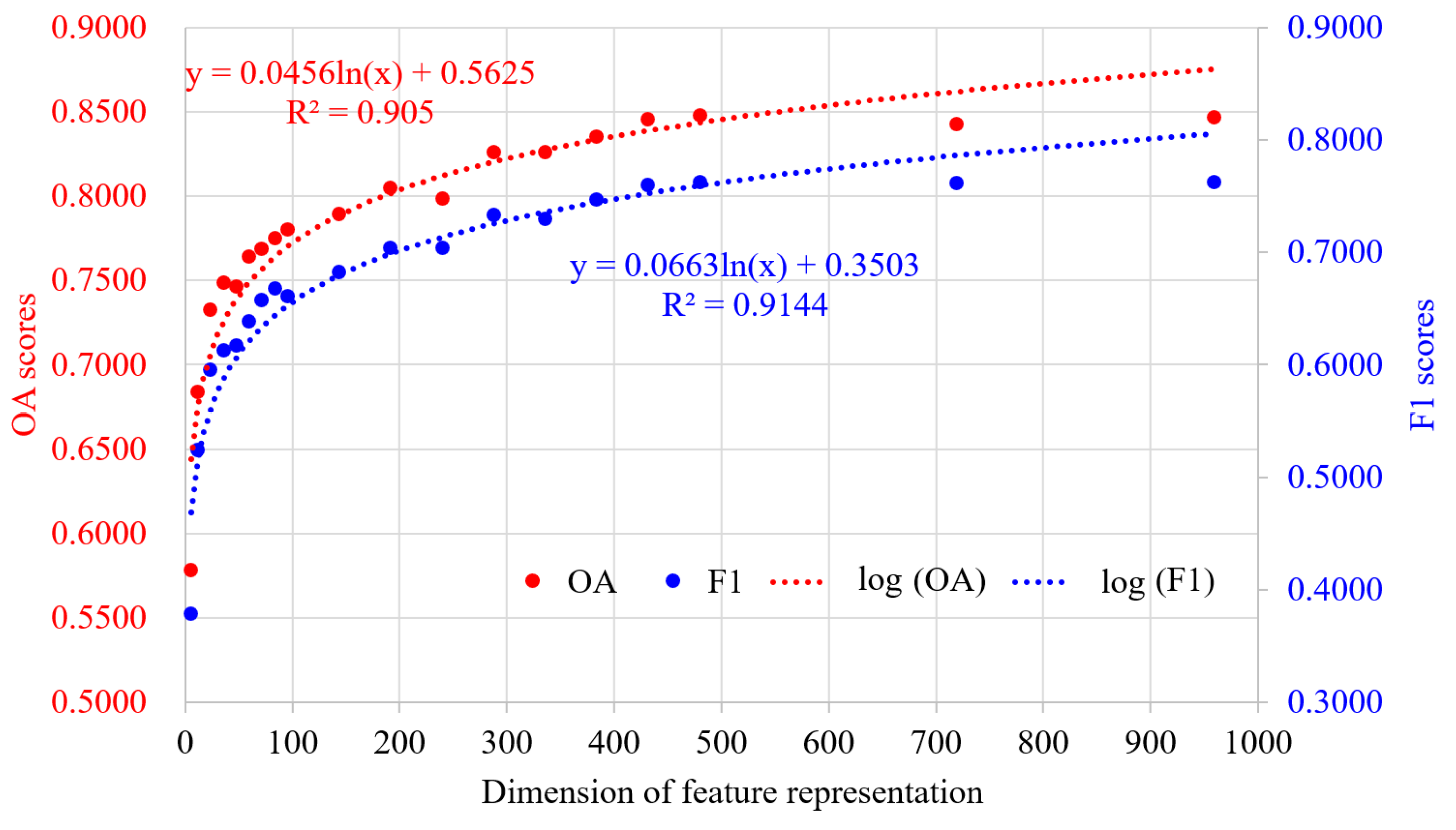
In time-series feature representation, the dimension of generated features is an important hyperparameter. If dimensions are too small, they cannot adequately convey the inherent characteristics of crop growth, whereas too-high dimensions could increase the amount of computation required for classification. In the Dijon study area, the contrastive learning framework produced features with dimensions of T/8, T/4, T/2, T, 2T, 3T, 4T, 5T, 6T, 7T, 8T, 9T, 10T, 15T, and 20T (T is the number of timestamps of raw time-series features, which is 48 in the Dijon study area). These features were used for time-series crop classification. Figure 8 illustrates classification accuracies (in OA and F1 scores) utilizing feature representations of varying dimensions.
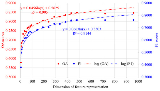
Figure 8.
Accuracy comparison along the dimension of feature representation.
4.1.6. Results on Vegetation Indices
Eight vegetation indices were derived to enhance crop mapping. Here, their contribution to crop classification was studied. In the Dijon study area, five comparative experiments were conducted, using (1) the 4-band image, (2) the vegetation index image (VI), (3) both the 4-band and 6-band images (10-band), (4) both the 4-band and vegetation index images (4 + VI), and (5) both the 10-band and VI images (10 + VI), respectively. The classification accuracies of various combinations of features are shown in Table 6.

Table 6.
Accuracy comparison for different combinations of features.
4.2. Discussion
The time-series feature representation based on contrastive learning was used to improve parcel-based crop mapping. First, classification performance in two study areas was compared and analyzed. Then, based on the parcel-based crop maps resulting from the XGB-FR classification, accuracy evaluations and comparisons were conducted to discuss the number of training samples, the benefit of type-wise contrastive learning, the sensitivity of dimensions in feature representation, and assistance from multitemporal composition and vegetation indices.
4.2.1. Performance Analysis
In two study areas, classification using time-series feature representation performed better than classification using raw time-series features. This indicated that the proposed contrastive learning framework could learn the inherent time-series characteristics of crop growth. In the meantime, it was observed that this proposed method performed better on the Zhaosu dataset than on the Dijon dataset. There are two reasons for this difference. One is that the crop category system in Zhaosu was more straightforward than its counterpart in Dijon. In addition, the sample category was more evenly distributed in the Zhaosu study area.
4.2.2. Number of Training Samples
Deep learning models typically require more labeled samples for training. Therefore, it is difficult to implement their applications in remote sensing fields when only a few samples are available. The proposed method (XGB-FR) is comprised two major steps. The first utilizes contrastive learning for the inherent representation of time-series spectral features. Although labeled crop types were used in the proposed type-wise contrastive learning, we could generate many augmented samples for training through type-wise random selection, random channel masking, and random timestamp masking. This step is not dependent on the number of labeled samples and does not need a massive quantity of samples. The second step is classification using XGBoost. It is a traditional machine-learning technique that only requires a small number of samples. However, LSTM-based classifiers contain a greater number of parameters, which requires more samples to train LSTM networks. Sample augmentation was, therefore, utilized in our experiments. Thus, the proposed XGB-FR method could learn and exploit the inherent time-series features of crop classification with a small number of training samples.
4.2.3. Type-Wise Contrastive Learning
In general, the accuracy scores in the last column in Table 4 indicate that classification using type-wise contrastive learning produced higher scores than those using instance-wise learning, with improvements in OA and F1 scores of 2.5% and 6.8%, respectively. This is evident since type-wise learning requires that samples with identical types share the same feature representation. This presumption necessitates contrastive learning to investigate the inherent characteristics of distinguishing crop types.
Let us examine the improvements made to various crops in further detail. We discovered a more substantial improvement in minor categories, specifically for ‘winter triticale’ (0.22), ‘sunflower’ (0.21), and ‘fallow’ (0.18), as measured using F1 scores. Possible causes include the fact that a loss function applied to positive sample pairs from two instances with the same crop types might reduce the inherent feature space of crops. Furthermore, the compression of space is more severe for major crop types than for minor types. These compressions would promote crop classification by balancing the distribution of the sample.
4.2.4. Need for Time-Series Composition
In Table 5, as the time intervals for time-series composition increased, the cloud/shadow coverage percentages decreased dramatically. Similarly, classification accuracies declined from 84.21% for OA and 0.76 for F1 scores when using 5-day raw data to 74.81% for OA and 0.58 for F1 scores when using 60-day composited data. This was somewhat surprising and contradictory to previous studies, which showed that the time-series monitoring of vegetation can be most effective when the composition period is near the length of phenological stages [43,44]. Since vegetation is usually assumed to be stable over 10 days [44], the best results should have been obtained utilizing a 10-day composition.
When investigating the causes, it was found that the time-series composition operation used satellite images captured on different days to produce one image. This could lead to the temporal confusion of crop growth in the composited image sequences, which is not favorable to crop classification. In addition, contrastive learning can fully explore the inherent time-series properties of raw data with a greater cloud/shadow percentage. In light of this, we may deduce that time-series composition is neither necessary nor detrimental in contrastive-learning-based feature representation.
4.2.5. Sensitive of the Dimension of Feature Representation
In Figure 8, the accuracy change curve can be separated into three phases as a whole. In the first stage (T/8 to 2T), classification accuracies improved as dimensions rose. This demonstrated that higher dimensions might capture more complete temporal changes in crop growth. In the second stage, from 2T to 9T, classification accuracy increased gradually. In the third stage (from 9T to 20T), classification accuracy remained consistent at the highest level, with an OA score of 84.78% and an F1 score of 0.7624. Thus, the 480-dimensional feature representation space may completely describe inherent crop characteristics. Here, we argue that the number of raw timestamps is an excellent candidate for determining the dimensions of represented features in crop classification.
4.2.6. Contributions of Vegetation Indices
In Table 6, it was found that classifications utilizing 10, 4 + VI, and 10 + VI characteristics yielded more accurate results than those using just 4 and VI features. The increase exceeded 9.0% for OA scores and 0.15 for F1 scores. This was expected, given that the 10, 4 + VI and 10 + VI features had more spectral information. In comparison to the 4-band feature, the VI feature demonstrated superior classification results. This is consistent with previous studies [45,46], demonstrating that red-edge spectral bands are sensitive to crop status. Comparing the 10-band classification to the 10 + VI classification, it was found that the contribution of VI features was minimal. This was because VI consists of non-linear combinations of the 10 spectral bands and is theoretically unnecessary. In addition, the contrastive learning framework could explore this information to improve classification. Thus, we recommend that raw spectral features be fed into the contrastive learning framework.
5. Conclusions
Fundamental to remote sensing crop mapping is extracting and learning inherent time-series features that can distinguish crop types from incomplete satellite observation sequences. This study developed a contrastive-learning-based framework for time-series feature representation to improve crop classification using incomplete Sentinel-2 image sequences. The proposed method is further discussed and validated through parcel-based time-series crop classifications in two study areas (one in Dijon of France and the other in Zhaosu of China) with multi-temporal Sentinel-2 images. The classification results, with significant improvements greater than 3% in their overall accuracy and 0.04 in F1 scores over comparison methods, revealed the effectiveness of the proposed method in learning time-series features for parcel-based crop classification using incomplete Sentinel-2 image sequences.
In addition, evaluations of accuracy and comparisons were performed on parcel-based classification results to discuss the number of training samples, the benefit of type-wise contrastive learning, the sensitivity of dimensions in feature representation, and assistance from time-series composition and vegetation indices. We concluded that (1) the combination of feature representation and traditional machine-learning-based classifications could improve parcel-based crop mapping with limited labeled samples. (2) Type-wise contrastive learning is more effective than instance-wise in time-series classification tasks. (3) Preprocessing time-series composition and vegetation indices is not necessary for contrastive-learning-based feature representation.
These experiments and their conclusion can provide insights and ideas for time-series classification in agricultural remote sensing applications. In addition, the proposed method is adaptable to other satellite images and applications in future works.
Author Contributions
Conceptualization, Y.Z. and N.Y.; methodology, Y.Z., N.Y. and L.F.; software, Y.W., L.F. and T.W.; validation, Y.W. and T.W.; formal analysis, Y.Z., Y.W. and L.F.; investigation, Y.W., N.Y. and Y.C.; resources, N.Y. and J.G.; data curation, Y.W., Y.C. and J.G.; writing—original draft preparation, Y.Z. and W.Z.; writing—review and editing, Y.Z. and N.Y.; visualization, Y.W., L.F. and X.Z.; supervision, Y.Z. and X.Z.; project administration, N.Y. and W.Z.; funding acquisition, Y.Z. and W.Z. All authors have read and agreed to the published version of the manuscript.
Funding
Please add: This research was funded by the Third Xinjiang Scientific Expedition Program, grant number 2021xjkk1305 and 2022xjkk0402, the National Key Research and Development Program of China, grant number 2019YFC1804301, and the National Natural Science Foundation of China, grant number 42071316 and 41901292.
Data Availability Statement
The data that support the findings of this study are available from the corresponding author upon reasonable request.
Acknowledgments
We thank the anonymous reviewers for their insights and constructive comments to help improve the paper.
Conflicts of Interest
The authors declare no conflict of interest.
References
- Huang, Y.; Chen, Z.; Tao, Y.; Huang, X.; Gu, X. Agricultural remote sensing big data: Management and applications. J. Integr. Agric. 2018, 17, 1915–1931. [Google Scholar] [CrossRef]
- Zhang, C.; Di, L.; Lin, L.; Li, H.; Guo, L.; Yang, Z.; Eugene, G.Y.; Di, Y.; Yang, A. Towards automation of in-season crop type mapping using spatiotemporal crop information and remote sensing data. Agric. Syst. 2022, 201, 103462. [Google Scholar] [CrossRef]
- Zhou, Y.; Luo, J.; Feng, L.; Yang, Y.; Chen, Y.; Wu, W. Long-short-term-memory-based crop classification using high-resolution optical images and multi-temporal SAR data. GIScience Remote Sens. 2019, 56, 1170–1191. [Google Scholar] [CrossRef]
- Liaghat, S.; Balasundram, S.K. A review: The role of remote sensing in precision agriculture. Am. J. Agric. Biol. Sci. 2010, 5, 50–55. [Google Scholar] [CrossRef]
- Yang, N.; Liu, D.; Feng, Q.; Xiong, Q.; Zhang, L.; Ren, T.; Zhao, Y.; Zhu, D.; Huang, J. Large-scale crop mapping based on machine learning and parallel computation with grids. Remote Sens. 2019, 11, 1500. [Google Scholar] [CrossRef]
- Rußwurm, M.; Körner, M. Self-attention for raw optical satellite time series classification. ISPRS J. Photogramm. Remote Sens. 2020, 169, 421–435. [Google Scholar] [CrossRef]
- Tatsumi, K.; Yamashiki, Y.; Torres, M.A.C.; Taipe, C.L.R. Crop classification of upland fields using Random forest of time-series Landsat 7 ETM+ data. Comput. Electron. Agric. 2015, 115, 171–179. [Google Scholar] [CrossRef]
- Zhou, Y.N.; Luo, J.; Feng, L.; Zhou, X. DCN-based spatial features for improving parcel-based crop classification using high-resolution optical images and multi-temporal SAR data. Remote Sens. 2019, 11, 1619. [Google Scholar]
- Yin, H.; Brandão, A., Jr.; Buchner, J.; Helmers, D.; Iuliano, B.G.; Kimambo, N.E.; Lewińska, K.E.; Razenkova, E.; Rizayeva, A.; Rogova, N. Monitoring cropland abandonment with Landsat time series. Remote Sens. Environ. 2020, 246, 111873. [Google Scholar] [CrossRef]
- Zhang, D.; Pan, Y.; Zhang, J.; Hu, T.; Zhao, J.; Li, N.; Chen, Q. A generalized approach based on convolutional neural networks for large area cropland mapping at very high resolution. Remote Sens. Environ. 2020, 247, 111912. [Google Scholar] [CrossRef]
- Chen, B.; Zheng, H.; Wang, L.; Hellwich, O.; Chen, C.; Yang, L.; Liu, T.; Luo, G.; Bao, A.; Chen, X. A joint learning Im-BiLSTM model for incomplete time-series Sentinel-2A data imputation and crop classification. Int. J. Appl. Earth Obs. Geoinf. 2022, 108, 102762. [Google Scholar] [CrossRef]
- Zhou, Y.N.; Wang, S.; Wu, T.; Feng, L.; Wu, W.; Luo, J.; Zhang, X.; Yan, N. For-backward LSTM-based missing data reconstruction for time-series Landsat images. GIScience Remote Sens. 2022, 59, 410–430. [Google Scholar] [CrossRef]
- Zhou, Y.N.; Yang, X.; Feng, L.; Wu, W.; Wu, T.; Luo, J.; Zhou, X.; Zhang, X. Superpixel-based time-series reconstruction for optical images incorporating SAR data using autoencoder networks. GIScience Remote Sens. 2020, 57, 1005–1025. [Google Scholar] [CrossRef]
- Garioud, A.; Valero, S.; Giordano, S.; Mallet, C. Recurrent-based regression of Sentinel time series for continuous vegetation monitoring. Remote Sens. Environ. 2021, 263, 112419. [Google Scholar] [CrossRef]
- Sun, L.; Gao, F.; Xie, D.; Anderson, M.; Chen, R.; Yang, Y.; Yang, Y.; Chen, Z. Reconstructing daily 30 m NDVI over complex agricultural landscapes using a crop reference curve approach. Remote Sens. Environ. 2021, 253, 112156. [Google Scholar] [CrossRef]
- Dong, J.; Xiao, X. Evolution of regional to global paddy rice mapping methods: A review. ISPRS J. Photogramm. Remote Sens. 2016, 119, 214–227. [Google Scholar] [CrossRef]
- Hu, Q.; Sulla-Menashe, D.; Xu, B.; Yin, H.; Tang, H.; Yang, P.; Wu, W. A phenology-based spectral and temporal feature selection method for crop mapping from satellite time series. Int. J. Appl. Earth Obs. Geoinf. 2019, 80, 218–229. [Google Scholar] [CrossRef]
- Jönsson, P.; Eklundh, L. TIMESAT—A program for analyzing time-series of satellite sensor data. Comput. Geosci. 2004, 30, 833–845. [Google Scholar] [CrossRef]
- Qiu, B.; Luo, Y.; Tang, Z.; Chen, C.; Lu, D.; Huang, H.; Chen, Y.; Chen, N.; Xu, W. Winter wheat mapping combining variations before and after estimated heading dates. ISPRS J. Photogramm. Remote Sens. 2017, 123, 35–46. [Google Scholar] [CrossRef]
- Vuolo, F.; Neuwirth, M.; Immitzer, M.; Atzberger, C.; Ng, W.-T. How much does multi-temporal Sentinel-2 data improve crop type classification? Int. J. Appl. Earth Obs. Geoinf. 2018, 72, 122–130. [Google Scholar] [CrossRef]
- Woźniak, E.; Rybicki, M.; Kofman, W.; Aleksandrowicz, S.; Wojtkowski, C.; Lewiński, S.; Bojanowski, J.; Musiał, J.; Milewski, T.; Slesiński, P. Multi-temporal phenological indices derived from time series Sentinel-1 images to country-wide crop classification. Int. J. Appl. Earth Obs. Geoinf. 2022, 107, 102683. [Google Scholar] [CrossRef]
- Hao, P.; Wang, L.; Zhan, Y.; Wang, C.; Niu, Z.; Wu, M. Crop classification using crop knowledge of the previous-year: Case study in Southwest Kansas, USA. Eur. J. Remote Sens. 2016, 49, 1061–1077. [Google Scholar] [CrossRef]
- Hao, P.; Wu, M.; Niu, Z.; Wang, L.; Zhan, Y. Estimation of different data compositions for early-season crop type classification. PeerJ 2018, 6, e4834. [Google Scholar] [CrossRef] [PubMed]
- Chu, D.; Shen, H.; Guan, X.; Chen, J.M.; Li, X.; Li, J.; Zhang, L. Long time-series NDVI reconstruction in cloud-prone regions via spatio-temporal tensor completion. Remote Sens. Environ. 2021, 264, 112632. [Google Scholar] [CrossRef]
- Chen, T.; Guestrin, C. Xgboost: A scalable tree boosting system. In Proceedings of the 22nd ACM Sigkdd International Conference on Knowledge Discovery and Data Mining, San Francisco, CA, USA, 13–17 August 2016; ACM: New York, NY, USA, 2016; pp. 785–794. [Google Scholar]
- Yuan, D.; Zhang, S.; Li, H.; Zhang, J.; Yang, S.; Bai, Y. Improving the gross primary productivity estimate by simulating the maximum carboxylation rate of the crop using machine learning algorithms. IEEE Trans. Geosci. Remote Sens. 2022, 60, 1–15. [Google Scholar] [CrossRef]
- Le-Khac, P.H.; Healy, G.; Smeaton, A.F. Contrastive representation learning: A framework and review. IEEE Access 2020, 8, 193907–193934. [Google Scholar] [CrossRef]
- Li, H.; Li, Y.; Zhang, G.; Liu, R.; Huang, H.; Zhu, Q.; Tao, C. Global and local contrastive self-supervised learning for semantic segmentation of HR remote sensing images. IEEE Trans. Geosci. Remote Sens. 2022, 60, 1–14. [Google Scholar] [CrossRef]
- Jaiswal, A.; Babu, A.R.; Zadeh, M.Z.; Banerjee, D.; Makedon, F. A survey on contrastive self-supervised learning. Technologies 2020, 9, 2. [Google Scholar] [CrossRef]
- Tang, C.I.; Perez-Pozuelo, I.; Spathis, D.; Mascolo, C. Exploring contrastive learning in human activity recognition for healthcare. arXiv 2020, arXiv:2011.11542. [Google Scholar]
- Zeng, Q.; Geng, J. Task-specific contrastive learning for few-shot remote sensing image scene classification. ISPRS J. Photogramm. Remote Sens. 2022, 191, 143–154. [Google Scholar] [CrossRef]
- Rußwurm, M.; Pelletier, C.; Zollner, M.; Lefèvre, S.; Körner, M. Breizhcrops: A time series dataset for crop type mapping. arXiv 2019, arXiv:1905.11893. [Google Scholar] [CrossRef]
- Wang, S.; Zhou, Y.N.; Yang, X.; Feng, L.; Wu, T.; Luo, J. BSNet: Boundary-semantic-fusion network for farmland parcel mapping in high-resolution satellite images. Comput. Electron. Agric. 2023, 206, 107683. [Google Scholar]
- Song, C.; Woodcock, C.E.; Seto, K.C.; Lenney, M.P.; Macomber, S.A. Classification and change detection using Landsat TM data: When and how to correct atmospheric effects? Remote Sens. Environ. 2001, 75, 230–244. [Google Scholar] [CrossRef]
- Chen, P.-Y.; Srinivasan, R.; Fedosejevs, G.; Kiniry, J. Evaluating different NDVI composite techniques using NOAA-14 AVHRR data. Int. J. Remote Sens. 2003, 24, 3403–3412. [Google Scholar] [CrossRef]
- Sun, Y.; Qin, Q.; Ren, H.; Zhang, T.; Chen, S. Red-edge band vegetation indices for leaf area index estimation from sentinel-2/msi imagery. IEEE Trans. Geosci. Remote Sens. 2019, 58, 826–840. [Google Scholar] [CrossRef]
- Herrmann, I.; Pimstein, A.; Karnieli, A.; Cohen, Y.; Alchanatis, V.; Bonfil, D. LAI assessment of wheat and potato crops by VENμS and Sentinel-2 bands. Remote Sens. Environ. 2011, 115, 2141–2151. [Google Scholar] [CrossRef]
- Richter, K.; Atzberger, C.; Vuolo, F.; Weihs, P.; D’Urso, G. Experimental assessment of the Sentinel-2 band setting for RTM-based LAI retrieval of sugar beet and maize. Can. J. Remote Sens. 2009, 35, 230–247. [Google Scholar] [CrossRef]
- Yue, Z.; Wang, Y.; Duan, J.; Yang, T.; Huang, C.; Tong, Y.; Xu, B. Ts2vec: Towards universal representation of time series. In Proceedings of the AAAI Conference on Artificial Intelligence, Online, 22 February–1 March 2022; Volume 36, pp. 8980–8987. [Google Scholar]
- Franceschi, J.-Y.; Dieuleveut, A.; Jaggi, M. Unsupervised scalable representation learning for multivariate time series. Adv. Neural Inf. Process. Syst. 2019, 32, 4650–4661. [Google Scholar]
- Tonekaboni, S.; Eytan, D.; Goldenberg, A. Unsupervised representation learning for time series with temporal neighborhood coding. arXiv 2021, arXiv:2106.00750. [Google Scholar]
- Foody, G.M. Status of land cover classification accuracy assessment. Remote Sens. Environ. 2002, 80, 185–201. [Google Scholar] [CrossRef]
- Holben, B.N. Characteristics of maximum-value composite images from temporal AVHRR data. Int. J. Remote Sens. 1986, 7, 1417–1434. [Google Scholar] [CrossRef]
- Julien, Y.; Sobrino, J.A. Comparison of cloud-reconstruction methods for time series of composite NDVI data. Remote Sens. Environ. 2010, 114, 618–625. [Google Scholar] [CrossRef]
- Forkuor, G.; Dimobe, K.; Serme, I.; Tondoh, J.E. Landsat-8 vs. Sentinel-2: Examining the added value of sentinel-2’s red-edge bands to land-use and land-cover mapping in Burkina Faso. GIScience Remote Sens. 2018, 55, 331–354. [Google Scholar] [CrossRef]
- Kaplan, G.; Avdan, U. Evaluating the utilization of the red edge and radar bands from sentinel sensors for wetland classification. Catena 2019, 178, 109–119. [Google Scholar] [CrossRef]
Disclaimer/Publisher’s Note: The statements, opinions and data contained in all publications are solely those of the individual author(s) and contributor(s) and not of MDPI and/or the editor(s). MDPI and/or the editor(s) disclaim responsibility for any injury to people or property resulting from any ideas, methods, instructions or products referred to in the content. |
© 2023 by the authors. Licensee MDPI, Basel, Switzerland. This article is an open access article distributed under the terms and conditions of the Creative Commons Attribution (CC BY) license (https://creativecommons.org/licenses/by/4.0/).


