Hyperspectral Prediction Model of Nitrogen Content in Citrus Leaves Based on the CEEMDAN–SR Algorithm

Abstract

Nitrogen content is one of the essential elements in citrus leaves (CL), and many studies have been conducted to determine the nutrient content in CL using hyperspectral technology. To address the key problem that the conventional spectral data-denoising algorithms directly discard high-frequency signals, resulting in missing effective signals, this study proposes a denoising preprocessing algorithm, complete ensemble empirical mode decomposition with adaptive noise joint sparse representation (CEEMDAN–SR), for CL hyperspectral data. For this purpose, 225 sets of fresh CL were collected at the Institute of Fruit Tree Research of the Guangdong Academy of Agricultural Sciences, to measure their elemental nitrogen content and the corresponding hyperspectral data. First, the spectral data were preprocessed using CEEMDAN–SR, Stein’s unbiased risk estimate and the linear expansion of thresholds (SURE–LET), sparse representation (SR), Savitzky–Golay (SG), and the first derivative (FD). Second, feature extraction was carried out using principal component analysis (PCA), uninformative variables elimination (UVE), and the competitive adaptive re-weighted sampling (CARS) algorithm. Finally, partial least squares regression (PLSR), support vector regression (SVR), random forest (RF), and Gaussian process regression (GPR) were used to construct a CL nitrogen prediction model. The results showed that most of the prediction models preprocessed using the CEEMDAN–SR algorithm had better accuracy and robustness. The prediction models based on CEEMDAN–SR preprocessing, PCA feature extraction, and GPR modeling had an $R^2$ of 0.944, $NRMSE$ of 0.057, and $RPD$ of 4.219. The study showed that the CEEMDAN–SR algorithm can be effectively used to denoise CL hyperspectral data and reduce the loss of effective information. The prediction model using the CEEMDAN–SR+PCA+GPR algorithm could accurately obtain the nitrogen content of CL and provide a reference for the accurate fertilization of citrus trees.

1. Introduction

Nitrogen is an essential nutrient for citrus trees, playing a crucial role in the production of vital compounds such as protein [1,2], chlorophyll, and enzymes, which substantially influence the growth, yield, and quality of citrus fruits [3,4]. Hence, accurate and timely assessment of nitrogen content in CL is crucial and can enable proper fertilization, to increase yields and fruit quality. It can also contribute to the reduction in excessive nitrogen application and the consequent pollution of surface water and groundwater [5,6].

Traditional methods of nitrogen analysis in plant leaves have used chemical techniques, which are time-consuming and require long detection periods [7,8]. Hyperspectral imaging is gaining popularity in agricultural engineering due to its integration of images and information [9,10]. It is capable of detecting the internal structure and external attributes of samples in a fast and nondestructive manner [11,12]. Costa et al. [13] developed a method for determining nutrient concentrations in citrus tree leaves using unmanned aerial vehicle (UAV) multispectral imagery and artificial intelligence techniques. Their gradient-enhanced regression-tree-based estimation model proved to be suitable for small sample data sizes and highly accurate in their study. Osco et al. [14] developed a machine learning framework for predicting nutrient content in CL, resulting in a $R^2$ as high as 0.912.

However, hyperspectral data unavoidably contain noise, due to extraneous information such as instrument dark currents, light scattering, and the baseline drift of the instrument during hyperspectral image capture. This adversely affects the accuracy and stability of model predictions [15,16]. Thus, many researchers have used filtering, wavelet, EMD, and other methods to preprocess the spectral data. Sharan et al. [17] processed Raman spectra using dual-density dual-tree complex wavelet transform with discrete wavelet transform, dual-tree complex wavelet transform, and the Savitzkv–Golav smoothing method. The results showed that the denoising method based on dual-density dual-tree complex wavelet transform improved the quantitative and qualitative analysis of Raman signals. Li et al. [18] used SG and FD to denoise spectral data in the preprocessing stage. They further filtered out the characteristic wavelengths using five different algorithms and created a prediction model based on Ls-SVM for predicting the chlorophyll content of lemon leaves, resulting in a best model $R^2$ value of 0.94 and a $RMSEP$ value of 0.10. As a result, denoising the spectral data of CL leads to more accurate model predictions.

Traditional filtering methods for processing hyperspectral data have problems such as the difficulty in resolving the local information of hyperspectral data and the ease of filtering out of the detailed part of the spectrum. The wavelet decomposition method decomposes the signal by predetermining the basis function, the number of decomposition layers, and the threshold selection method, which requires a lot of time for experimental testing and is a troublesome process. The EMD algorithm is based on the scale of the data itself, but there is a mode mixing problem. As a result, many researchers have focused on improving the EMD algorithm.Tang et al. [19] proposed a preprocessed algorithm with EEMD-db3 for noise reduction to process PsR spectral data. The method effectively improves the signal-to-noise ratio and enhances the relationship between the spectral data and heavy metal content. The algorithm also enhances the stability and accuracy of the estimation model. In a similar vein, Zhao et al. [20], processed the Raman spectra of rice plants using EMD, EEMD, and complementary ensemble empirical mode decomposition (LCEEMD) methods, to establish a neural network prediction model. The LCEEMD method not only solves the modal mixing problems of high-frequency signals and noise in EMD but also effectively reduces residual noise in EEMD. Currently, EMD-like algorithms are not widely used in the nondestructive detection of nutrient content in CL, and there are few preprocessing algorithms based on EMD-like algorithms available.

Sparse representation based on compressed perception overcomes the limitations of traditional sampling theory and processes information from the perspective of sparse representation, which is widely used in the fields of image processing, speech recognition, natural language processing, etc. [21], and has a high computational efficiency and practicality. Some scholars have tried to denoise hyperspectral signals with sparse representation, and they found that the sparse representation method is better for spectral signals with a low signal-to-noise ratio and weaker for spectral signals with a high signal-to-noise ratio. Fang et al. [22] proposed a method for recovering the peak information of high-noise Raman signals based on joint sparse representation. This method uses the sparsity of the Raman spectrum to recover the signals and preserve useful peak information. The peak information is then reconstructed using an orthogonal matching pursuit algorithm. The joint sparse representation method can effectively analyze Raman spectra, especially those with a high noise level. Experimental results showed that the method outperforms other methods at low signal-to-noise ratios. Guo et al. [23] proposed a 1-dD denoising method for water color hyperspectral data based on sparse representation. The method was found to be effective, but the sparse representation also destroyed some of the useful information at higher signal-to-noise ratios.

This study proposes an adaptive denoising preprocessing algorithm for hyperspectral data from CL using the CEEMDAN–SR algorithm. The proposed method effectively reduces noise, retains effective information, and improves the signal-to-noise ratio of the spectral signal. Initially, the CEEMDAN–SR, SURE–LET, SR, SG, and FD algorithms were employed to denoise the hyperspectral data of the CL. Then, the PCA, UVE, and CARS algorithms were used for feature selection. Finally, PLSR, SVR, RF, and GPR were used to construct a model for predicting nitrogen content in CL.

The main contributions of this paper are as follows:

1.

A CEEMDAN–SR algorithm is proposed that can denoise the raw hyperspectral data of CL in the preprocessing stage. The algorithm improves the signal-to-noise ratio of spectral data by removing high-frequency noise, while retaining most of the effective information. The CEEMDAN–SR, SURE–LET, and SR algorithms are experimentally demonstrated for use as denoising algorithms for CL hyperspectral data in the preprocessing stage;

2.

Based on the characteristics of CL hyperspectral data, a quantitative analysis was carried out to establish a model for predicting the nitrogen content of CL. The CEEMDAN–SR+PCA+GPR prediction model has a strong fitting effect and accuracy, with low error, and can be used for rapid nondestructive detection of nitrogen content in CL.

2. Materials and Methods

2.1. Study Area

The CL were collected on 30 September 2022, from the Institute of Fruit Tree Research of the Guangdong Academy of Agricultural Sciences, as indicated in Figure 1. Samples were taken from three different citrus seedlings, namely, Gongkang, Satsuma, and Wogan. A total of 75 sets of samples were collected from each species, resulting in 225 sets of samples. Each tree was divided into three parts: top, middle, and bottom. Healthy and fresh leaves were collected from the 3rd or 4th layer in four directions, from southeast to northwest, and from top to bottom. The collected leaves were thoroughly washed with water to remove any dust and dirt, dried with a clean cotton cloth, placed in fresh bags, numbered, and transported to the laboratory immediately for further processing.

2.2. Hyperspectral Data Acquisition and Nitrogen Content Determination

The study employed a GaiaField-F-V10 portable feature hyper-spectrometer as the acquisition instrument for hyperspectral reflectance data. This hyper-spectrometer is composed of three components, namely, an imaging lens, an imaging spectrometer, and a surface array detector. These components are illustrated in Figure 2.

The hyper-spectrometer has a spectral range of 400–1000 nm, a spectral resolution of 3.8 nm, and 256 spectral channels. To ensure that the data obtained were accurate, three separate photographs were taken of each set of samples using the hyper-spectrometer, which was positioned in a dark box and illuminated by a halogen lamp. In this dark box, the white reference image was obtained by scanning a standard white ceramic plate, the black reference image was obtained by scanning the lens cover over the lens cap, and then the original hyperspectral image was calibrated according to Formula (1). Figure 3 shows a flowchart for extracting the reflectance curve by sequentially reading and mask segmenting 256 channels of CL hyperspectral images using OpenCV.

$$I_0=\frac{I-I_D}{I_W-I_D}$$

(1)

where $I_0$ is the calibrated image, I is the raw image, $I_W$ is the white reference image, and $I_D$ is the dark reference image.

The fresh CL were dried and ground using the Naive calorimetry method to determine their total nitrogen content. Abnormal data were removed from the measured nitrogen content of CL using the box plot method, to restore objectivity for a better analysis. This was necessary because the CL chemistry measurement method is prone to errors caused by testers, operations, and other factors.

Table 1. Statistical table of CL nitrogen content data after excluding abnormal data.

	Count	Mean/%	Standard Deviation/%	Min/%	Max/%
N	215	2.499	0.596	0.966	3.920

shows the statistical data of the nitrogen content of the CL after the removal of abnormal data.

2.3. Spectra Pretreatment

2.3.1. Traditional Methods

SG is a polynomial smoothing algorithm based on the principle of least squares, proposed by Savitzkg and Golag, which is widely used in spectral preprocessing [24]. The FD transform is likewise a common method of spectral preprocessing that highlights the rate of increase or decrease in spectral reflectance [25].

2.3.2. SURE–LET

The SURE–LET algorithm, proposed by SteinLuisier et al. [26], employs unbiased risk estimation (SURE) and linear expansion of thresholds (LET) to determine the optimal threshold in wavelet-based denoising problems. SURE–LET solves for the optimal weights of the denoising results of different shrinkage basis functions using a system of linear equations, which can be used for denoising a signal, image, video, etc. [27,28].

2.3.3. CEEMDAN

The complete ensemble empirical mode decomposition with adaptive noise (CEEMDAN) algorithm, introduced by Torres et al. in 2011, addresses the limitations of EMD [29]. EMD is vulnerable to modal mixing, as highlighted in prior research [30,31]. Unlike the EEMD and CEEMD algorithms, CEEMDAN effectively isolates residual noise and suppresses any added white noise signals. The CEEMDAN algorithm adds Gaussian white noise to the intrinsic mode function (IMF) components post-EMD decomposition and then computes an overall average calculation following the first-order IMF, to generate the final first-order IMF. This process is repeated for the residual component until the residual signal is transformed into a monotonic function and cannot be decomposed further. Hence, the noise transfer from high to low frequencies is effectively addressed. Let $E_i$ denote the ith eigenmode component obtained post-EMD decomposition, and let the ith eigenmode component obtained via CEEMDAN decomposition be $\overline{IM{F}_1\left(t\right)}$. Let $v^j$ be the Gaussian white noise signal conforming to the standard normal distribution, $\epsilon$ be the standard deviation of the noise, and $z\left(t\right)$ be the original signal. The CEEMDAN decomposition process involves the following steps:

1.

A new signal $z\left(t\right)+{(-1)}^q\epsilon v^j$ is obtained by adding positive and negative paired Gaussian white noise to the original signal $z\left(t\right)$, where q = 1 or 2. The EMD decomposition of the new signal yields the first-order IMF component $IM{F}_1$, as shown in Formula (2):

$$E\left(z\left(t\right)+{(-1)}^q\epsilon v^j\right)=IM{F}_1^j\left(t\right)+r^j$$

(2)

2.

The N IMF components generated are summed and averaged, as shown in Formula (3):

$$\overline{IM{F}_1\left(t\right)}=\frac{1}{N}\sum _{j=1}^{N}IM{F}_1^j\left(t\right)$$

(3)

3.

T residuals are calculated after removing the first IMF component, as shown in Formula (4):

$$r_1\left(t\right)=z\left(t\right)-\overline{IM{F}_1\left(t\right)}$$

(4)

4.

A new signal is obtained by adding positive and negative pairwise Gaussian self-noise to $r_1\left(t\right)$, and this new signal is used as a carrier for EMD decomposition, to obtain the 1st IMF component $D_1^j$, from which the 2nd IMF component can be obtained, as shown in Formula (5):

$$\overline{IM{F}_2\left(t\right)}=\frac{1}{N}\sum _{j=1}^N{D}_1^j\left(t\right)$$

(5)

5.

The residuals are calculated with the second IMF component removed, as shown in Formula (6):

$$R^2\left(t\right)=r_1\left(t\right)-\overline{IM{F}_2\left(t\right)}$$

(6)

6.

The above steps are repeated until the residual signal obtained is a monotonic function and cannot be further decomposed. At this point, the number of IMF components obtained is K, and the original signal $z\left(t\right)$ is then decomposed into K IMF and one residual, as shown in Formula (7).

$$z\left(t\right)=\sum _{k=1}^K\overline{IM{F}_K\left(t\right)}+r_K\left(t\right)$$

(7)

2.3.4. SR

Sparse representation (SR) is a method of representing a signal as a linear combination of a set of basis vectors, where very few basis vectors are involved in the linear combination, and thus this allows for compression and denoising of the signal [32,33]. The sparse redundant representation model based on an overcomplete dictionary assumes that any signal x can be represented by as sparse a vector $\alpha$ as possible under a dictionary D consisting of atoms, as shown in Formula (8):

$$x=D\alpha$$

(8)

Therefore, the method of reconstructing the original signal x mainly involves the dictionary D and the sparse vector $\alpha$. In order to achieve a sparse representation of the signal, the optimal sparsity must be solved to approximate the original signal, assuming that D is known, which can be expressed in the above model as Formula (9):

$$\alpha ={argmin\parallel \alpha \parallel }_0\mathrm{s}.\mathrm{t}.x=D\alpha$$

(9)

where ${\parallel \alpha \parallel }_0$ denotes the ${ł}_0$ paradigm, which is used to constrain the number of individual non-zero terms in the sparse vector.

From the above analysis, it can be seen that the construction of a sparse representation model based on an overcomplete dictionary is mainly achieved by designing a better overcomplete dictionary D and obtaining a better sparse vector $\alpha$. In this paper, we adopt the SR method to select the DCT discrete cosine transform as a fixed orthogonal dictionary using the orthogonal matching pursuit (OMP) algorithm as a way to solve the sparse vectors. The OMP algorithm is a greedy algorithm used to solve a system of sparse linear equations [34,35]. This algorithm gradually constructs an overcomplete dictionary matrix by searching for the variable that best explains the remaining unexplained observations at each selection step.

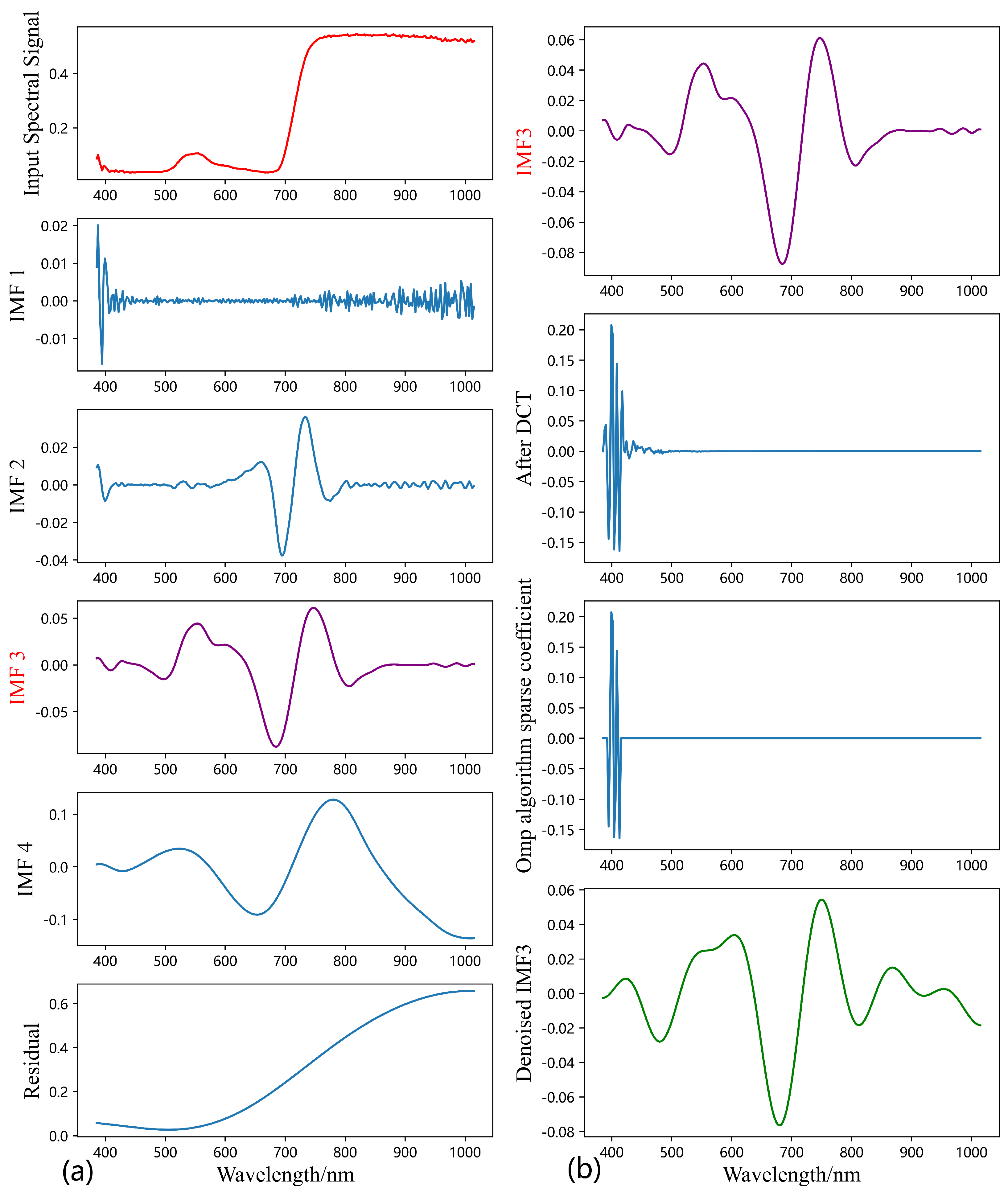
2.3.5. CEEMDAN–SR

Although the CEEMDAN algorithm can decompose the signal adaptively according to its own characteristics, if it is not differentiated and the entire component is denoised, the removal of noise will also take away some of the useful signals.

A novel denoising algorithm called complete ensemble empirical mode decomposition with adaptive noise joint sparse representation (CEEMDAN–SR) is proposed in this study. The CEEMDAN algorithm is introduced to adaptively decompose the original spectral signals to obtain n IMFs, which are filtered by combining the correlation coefficient and the adaptive thresholding method based on the variance contribution ratio. Subsequently, the SR algorithm is used to denoise the eigenmode functions that contain more noise and less valid information, and finally CEEMDAN reconstruction is performed. The algorithm can effectively accomplish the task of removing noise from noisy spectral signals and retain key information. The steps for implementing the CEEMDAN–SR algorithm are as follows:

1.

Input the original spectral signal X. CEEMDAN decomposition of X is performed to obtain a set of eigenmode functions $S_1$ containing n IMFS and a residual $\epsilon$;

2.

Solve for the correlation coefficient r with the input signal X for each IMF in the set $S_1$, as shown in Formula (10):

$$r=\frac{{\sum }_{i=1}^m(IM{F}_t\left(i\right)-I\overline{M}{F}_t)(X\left(i\right)-\overline{X})}{\sqrt{{\sum }_{i=1}^m{(IM{F}_t\left(i\right)-I\overline{M}{F}_t)}^2}\sqrt{{\sum }_{i=1}^m{(X\left(i\right)-\overline{X})}^2}}$$

(10)

where $IM{F}_t$ represents the t-th element in $S_1$, $I\overline{M}{F}_t$ represents the mean value of the $IM{F}_t$, $\overline{X}$ represents the mean value of the original spectral signal X, and m represents the number of bands of the spectrum, where in this paper $m=256$;

3.

Referring to the EMD improvement algorithm proposed by Lin et al. [36], this paper selects 0.1 as the correlation coefficient threshold. For IMFs with a correlation coefficient less than 0.1, they are regarded as pseudo-IMF components and are not involved in signal reconstruction. The IMFs with correlation coefficients less than 0.1 in $S_1$ are discarded, to obtain the set $S_2$;

4.

For the elements in $S_2$, solve for their adaptive threshold based on their variance contribution, as shown in Formulas (11) and (12):

$$\left\{\begin{array}{c}{K}_t=\frac{1}{n}\sum _{t=1}^n{\left(IM{F}_t\right)}^2-{\left[\frac{1}{n}\sum _{t=1}^{n}IM{F}_t\right]}^2\hfill \\ C_t=\frac{K_t}{{\sum }_{t=1}^n{K}_i}\times 100\%\hfill \end{array}\right.$$

(11)

$$\mathrm{threshold}=\frac{1}{n}\sum _{t=1}^n{C}_t-0.5\times \sqrt{\frac{1}{n}\sum _{t=1}^n{\left(C_t-\frac{1}{n}\sum _{t=1}^n{C}_t\right)}^2}$$

(12)

where n represents the number of elements in $S_2$, $IM{F}_t$ represents the t-th element in $S_2$, $K_t$ is the variance of $IM{F}_t$, and $C_t$ is the contribution of the variance of the $IM{F}_t$.

5.

The elements of $S_2$ whose threshold are less than 0.3 are denoised using the SR algorithm to obtain set $S_3$;

6.

The CEEMDAN reconstruction of $S_3$ and the residual $\epsilon$ is performed to obtain the reconstructed signal Y;

7.

Output the denoised spectral signal Y.

Figure 4a shows a schematic diagram of the decomposition of the original spectral profile using the CEEMDAN algorithm. It can be seen that the original spectral profile is decomposed into four IMFs: IMF1, IMF2, IMF3, and IMF4, and one residual. Combining the correlation coefficient and the adaptive thresholding method based on the variance contribution ratio, it is judged that IMF3 needs to be denoised. The denoising process of IMF3 using the sparse representation is shown in Figure 4b.

2.4. Feature Extraction Methods

The PCA, UVE, and CARS algorithms were selected as the feature extraction algorithms for the CL hyperspectral data [37,38,39], and the results of the three algorithms for the feature extraction of the original spectral curves processed by the CEEMDAN–SR algorithm are shown in Figure 5a. Figure 5a shows a schematic diagram of the PCA algorithm processing, where a total of 16 principal components were extracted, the explained variance of the first principal component was as high as 0.751, and the first 16 principal components basically contained 99.9% of the information of the original spectrum. Figure 5b shows a schematic diagram of the UVE algorithm used to eliminate the uninformative bands and retain the effective bands, and the vertical red line position indicates the effective bands retained. Figure 5c shows the result of the Monte Carlo sampling number of the 50 Cars algorithm on the spectral data downscaling, where the red dot position is the minimum value of RMSECV.

2.5. Model Building and Evaluation Methods

Four regression algorithms were selected to construct the CL nitrogen content prediction model.The algorithms used were partial least squares regression in a linear model, support vector machine regression in a non-linear model, random forest regression in an integrated regression model, and Gaussian process regression in a probabilistic model based on Bayesian regression.

Table 2. A brief introduction to the modeling algorithms used in this study.

Methods	Description	Reference
Partial least squares regression (PLSR)	PLSR is a linear model that aims to find latent variables that capture the maximum covariance between the predictor variables and the response variable, allowing for efficient modeling of complex relationships and handling of multicollinearity.	[40]
Support vector regression (SVR)	SVR is a supervised learning algorithm that utilizes support vector machines to perform regression tasks by finding an optimal hyperplane that maximizes the margin, while minimizing the error between the predicted and actual values.	[41]
Random forest (RF)	RF is an ensemble learning method that combines multiple decision trees to predict the response variable by averaging the predictions of individual trees.	[42]
Gaussian processes regression (GPR)	GPR is a probabilistic regression model that uses a collection of data points to estimate an underlying function by assuming a Gaussian distribution over possible functions, enabling flexible predictions and uncertainty quantification.	[43]

provides a brief description of each regression algorithm.

In order to objectively assess the modeling accuracy, we partitioned the dataset using the SPXY algorithm. We selected 4/5 of the samples for modeling and 1/5 for validation. The SPXY algorithm is an improved method based on the KS algorithm. It partitioned the dataset by calculating the Euclidean distance in both the x and y-vector directions for different samples. This approach combines the distances in the x and y directions through regularization, resulting in a more comprehensive evaluation and partitioning of the dataset.

The coefficient of determination $R^2$, normalized root mean squared error ($NRMSE$), and residual predictive deviation ($RPD$) were chosen as the evaluation indicators for the model. Their expressions are shown in Formulas (13)–(15):

$$R^2=\frac{{\sum }_{i=1}^m\left({\widehat{y}}_i-{\overline{\widehat{y}}}_i\right)\left(y_i-\overline{y}\right)}{\sqrt{{\sum }_{i=1}^m{\left({\widehat{y}}_i-{\overline{\widehat{y}}}_i\right)}^2}\sqrt{{\sum }_{i=1}^m{\left(y_i-\overline{y}\right)}^2}}$$

(13)

$$NRMSE=\sqrt{\frac{{\sum }_{i=1}^m{\left(y_i-{\widehat{y}}_i\right)}^2}{m\times {(y_{min}-y_{min})}^2}}$$

(14)

$$RPD=\sqrt{\frac{{\sum }_{i=1}^m{\left(y_i-\overline{y}\right)}^2}{{\sum }_{i=1}^m{\left(\widehat{y_i}-y_i\right)}^2}}$$

(15)

where $y_i$ and ${\widehat{y}}_i$ are the true and predicted values of CL sample i, m represents the number of predicted samples, $\overline{y}$ is the mean of the true values, and ${\overline{\widehat{y}}}_i$ is the mean of the predicted values. $y_{max}$ and $y_{min}$ represent the maximum and minimum values of the true value. A higher $R^2$ value indicates a better degree of fitting of the model, and a smaller $NRMSE$ value indicates a higher accuracy of the prediction model. A model with $RPD$ values lower than 1.5 is deemed inadequate, while those with $RPD$ above 2.0 are considered to have good robustness.

3. Results

3.1. Comparison of the Denoising Effect of Different Preprocessing Methods

A random strip of spectral reflectance in the wavelength range of 400–1000 nm was selected for each of the three CL varieties. Spectral reflectance data for the three citrus varieties are presented in Figure 6. The spectral reflectance trends of the three citrus varieties exhibited a consistent pattern, with a reflectance peak at approximately 549 nm and an absorption trough at around 678 nm, followed by a sharp increase in reflectance in the subsequent bands, and a maximum value at 760 nm. Eventually, there was a slight decrease in reflectance towards the higher wavelength end. The reflectance peaks of the three citrus varieties were obscured by noise in most bands, especially in the green band at approximately 549 nm. This noise-covered signal contain errors and potentially reduce the accuracy of the regression predictions.

We preprocessed a randomly chosen set of spectral reflectances of CL using four different methods, namely CEEMDAN–SR, SURE–LET, SR, and CEEMDAN. The results of the preprocessing are illustrated in Figure 7.

According to Figure 7, the spectral curves of all four images following denoising were relatively smooth, suggesting that all four methods effectively removed burrs and rejected noise. Comparing the waveforms prior to and post noise reduction (Figure 7a), it can be observed that the pure signal subjected to the CEEMDAN–SR denoising method was closest to the original spectral curve. The preserved peaks, positions of peaks and troughs, and the overall resemblance to the original spectrum indicate the efficacy of the method in eliminating noise information, while retaining the relevant data. Figure 7b,c show that the SURE–LET and SR methods effectively denoised most of the spectral characteristics, but did not resolve spectral details well, resulting in some deviations from the original spectral curves in several bands. For instance, the spectral curve processed by the SURE–LET method experienced a shift in peak position, and the value of the reflection peaks at 500–600 nm and did not match the original spectral curve at 600–700 nm. Likewise, the SR method did not perform better, as it demonstrated inadequate treatment near the trough at 600–660 nm, leading to a shift in peak position and value. Figure 7d shows that the CEEMDAN method provided unsatisfactory results. The spectral curve processed using the CEEMDAN algorithm significantly deviated from the original spectral curves across the entire wavelength range, with the replicated peak and trough positions and values not recovering from the noise. This occurred due to the CEEMDAN algorithm’s removal of IMFs with low correlation, which removed the noise but also discarded useful information, leading to unsatisfactory results.

Figure 8 displays the average waveform similarities between the denoised curves and the original spectral curves obtained from the four denoising algorithms. The values were computed from 100 randomly selected spectral curves. Formula (16) defines the $NCC$ (Normalized Correlation Coefficient) expression.

$$NCC(x,y)=\frac{{\sum }_{i=1}^n\left(x_i-\overline{x}\right)\left(y_i-\overline{y}\right)}{\sqrt{{\sum }_{i=1}^n{\left(x_i-\overline{x}\right)}^2}\sqrt{{\sum }_{i=1}^n{\left(y_i-\overline{y}\right)}^2}}$$

(16)

where x and y are the original spectral curve and denoised spectral curve, n is the number of samples in each curve, and $\overline{x}$ and $\overline{y}$ are the means of the original spectral curve and denoised spectral curve. The larger the $NCC$, the better the denoising effect.

The CEEMDAN–SR algorithm had a waveform similarity coefficient of 0.9981, which was significantly higher than that of all other algorithms, which had coefficients lower than 0.99. Hence, utilization of the CEEMDAN–SR algorithm for noise reduction led to a considerable improvement in the decreasing the distortion of the characteristic peaks of the spectral curve and in restoring the spectral absorption characteristics of the CL.

3.2. Construction of Prediction Models for CL Nitrogen Content

We used CEEMDAN–SR, SURE–LET, SG, FD, and SR as preprocessing methods; PCA, UVE, and CARS to select feature bands; and PLSR, SVR, RF, and GPR from the commonly used hyperspectral prediction models for CL nitrogen prediction modeling.

The results of the model evaluation metrics are shown in Figure 9. The first row shows the values of the individual combined model decision coefficients $R^2$, the second row shows the values of $NRMSE$, and the third row shows the values of $RPD$.

According to Figure 9, it was found that the CEEMDAN–SR method was the most effective denoising algorithm in modeling the nitrogen content of CL compared to the other four methods. The predictions for all combinations of feature selection and modeling methods performed better than the other four algorithms, except for the combination of CARS+RF, which had an unsatisfactory overall performance. The $R^2$ values were all greater than 0.8, the $NRMSE$ values were all less than 0.1, and the $RPD$ values were all greater than 2.0, indicating a good fit for effective modeling. When excluding the combination of the CARS+RF and UVE+RF algorithms and comparing the remaining combinations, the CEEMDAN–SR method was found to model the highest $R^2$ and $RPD$ values among the five denoising algorithms and the smallest $NRMSE$ among all five. In conclusion, the CEEMDAN–SR method can be considered an effective method to establish a prediction model for CL nitrogen content, with both stability and accuracy.

All combinations, except CEEMDAN–SR, that were preprocessed using the SR method exhibited satisfactory performance. The seven combinations, namely SR+PCA+PLSR, SR+PCA+SVR, SR+PCA+GPR, SR+UVE+PLSR, SR+UVE+GPR, SR+CARS+PLSR, and SR+CARS+SVR, had an $R^2$ value exceeding 0.8. In addition, they had a smaller value of $NRMSE$ and a larger value of $RPD$. Preprocessing the data with the SURE–LET algorithm, improved the performance of the combinations SURE–LET+PCA+SVR, SURE–LET+PCA+GPR, and SURE–LET+UVE+GPR. These combinations exhibited an $R^2$ value exceeding 0.8, a smaller $NRMSE$ value, and a larger $RPD$ value, fitting the data better.

Traditional preprocessing algorithms were compared using SG and FD methods. The SG algorithm was more efficient and provided a good fit for data, while the FD method did not perform well for preprocessing combinations. The SG algorithm offered three combinations: SG+PCA+GPR, SG+UVE+RF, and SG+UVE+GPR, all with $R^2$ values greater than 0.8, $NRMSE$ less than 0.1, and $RPD$ greater than 2. As for the FD algorithm, most of the combinations had $R^2$ values between 0.6 and 0.7, and only two, FD+PCA+SVR and FD+CARS+RF, had $R^2$ values below 0.6. Using the FD method as the pretreatment method resulted in $RPD$ values less than 2 and higher $NRMSE$ values compared to the other four pretreatment methods, leading to an unsatisfactory fit, a weak explanatory power of the model, and poor prediction results.

The most effective combination of the five denoising algorithms was selected for model fit analysis and residual analysis, to indicate the fit of the predictive model and the accuracy of the predicted values, as shown in Figure 10.

Figure 10a,b show the CEEMDAN–SR+PCA+GPG combination with an $R^2$ of 0.944, $NRMSE$ of 0.057, and $RPD$ of 4.219, which was the best fit for CL nitrogen content and predicted with a much higher accuracy than the best combination of the other four denoising algorithms. This suggests that the CEEMDAN–SR method can better remove invalid noise and retain valid information compared to the other noise reduction methods. The model built using the CEEMDAN–SR preprocessing method was better fitted to the regression, and the predicted data deviated less from the true values.

Figure 10c–h present three modeling combinations for the SURE–LET, SR, and SG denoising algorithms as SURE–LET+PCA+GPR, SR+PCA+GPR, and SG+UVE+GPR, respectively, which performed well in predicting the CL nitrogen content, with small errors between the predicted and actual values. The results suggest that the SURE–LET, SR, and SG methods are reliable pretreatment methods for predicting nitrogen content in CL.

Among the preprocessing models considered, the FD preprocessed model presented the worst performance, as seen in Figure 10i,j. The best-performing combination of FD+UVE+GPR resulted in an $R^2$ of 0.725, $NRMSE$ of 0.121, and $RPD$ of 1.906, indicating a poor fit with the data, with a substantial deviation between the predicted and actual values.

The average memory space required and the average time spent for the prediction of a single CL spectral curve by the best modeling combinations of the above five classes of preprocessing algorithms are given in

Table 3. Memory space required and time spent for the five types of denoising algorithms best combined models.

Models	Average Memory Space Required/Mib	Average Time Spent/s
CEEMDAN–SR+PCA+GPR	180.023	2.046
SURE–LET+PCA+GPR	176.484	1.238
SR+PCA+GPR	179.539	1.207
SG+UVE+GPR	176.847	1.256
FD+UVE+GPR	176.882	1.247

. It can be seen that they were similar in terms of the memory space required for execution, which was about 180 Mib, but there was a large difference in terms of runtime. Among them, the CEEMDAN–SR+PCA+GPR model predicted a longer time of 2.046 s, while the other four types of model were all around 1.2 s.

4. Discussion

4.1. Analysis of the Denoising Ability of the Preprocessing Algorithms

The disadvantage of the SR algorithm in processing spectral data lies in the fact that denoising signals with a high signal-to-noise ratio will take away part of the relevant information. In this study, the CEEMDAN algorithm, combined with the correlation coefficient and the adaptive thresholding method based on the variance contribution ratio, could decompose the spectral data and then filter out the IMFs containing more noise and less useful information; that is, those with lower signal-to-noise ratios, to be processed by the SR algorithm. This protected against the loss of relevant information and improved the signal-to-noise ratio of the spectral data. As shown in Section 3.1, CEEMDAN–SR effectively eliminated noise, while preserving peak values and positions in the reflection peaks. Wang et al. [44] stated that the NCC shows the difference between the denoised and original spectra. The lower the difference, the more useful information is retained and the better the denoising effect. Compared to the SURE–LET, SR, and CEEMDAN methods, the CEEMDAN–SR algorithm produced the highest waveform similarity between the preprocessed and original spectral profiles.

The results demonstrated that hyperspectral data preprocessed using the CEEMDAN–SR algorithm provided better modeling than traditional denoising algorithms. Of the twelve feature selection and modeling combinations tested, the combination of CEEMDAN–SR, PCA, and GPR produced the best model fit and the smallest prediction error. This combination yielded an $R^2$ of 0.944, $NRMSE$ of 0.057, and $RPD$ of 4.219, with high robustness. The results indicated that the CEEMDAN–SR algorithm is both applicable and stable in the denoising stage of CL hyperspectral data, and that it can be utilized as a suitable denoising algorithm for this type of data. Specifically, 10 out of the 12 feature selection and modeling combinations achieved an $R^2$ greater than 0.8, $RPD$ greater than 2, and smaller $NRMSE$, demonstrating the superior performance of the CEEMDAN–SR algorithm in comparison to the other algorithms. Both EMD-like algorithms and wavelet decomposition are capable of decomposing a noisy signal into multiple components and denoising the components that contain the most noise. Unlike the EMD algorithm, CEEMDAN can decompose spectral signal modes into a series of IMF components with frequencies ranging from high to low. This eliminates the mode mixing problem and provides superior modal spectrum separation when compared to EEMD, avoids spurious IMF components, and further improves the mode mixing effect. It is expected that future research will prioritize the CEEMDAN algorithm and its combinations with other algorithms for spectral data processing applications.

The SURE–LET and SR algorithms are widely used in image denoising but not as much in hyperspectral data denoising. From the experimental results Section 3.2 it can be seen that the SURE–LET algorithm had two combinations of $R^2$ greater than 0.8, and the SR algorithm had seven combinations of $R^2$ greater than 0.8, with larger values for $RPD$ and smaller values for $NRMSE$. However, SURE–LET has the disadvantage that it is difficult to determine the number of layers of the wavelet decomposition and the wavelet basis function, and although SURE–LET performs adaptive thresholding, some useful high-frequency information is filtered out while the high-frequency part is filtered. Therefore, SURE–LET loses useful information in the spectral signal, while suppressing spectral noise, resulting in large changes in spectral peaks and peak positions [45,46,47]. The SR algorithm is based on the principle of representing the signal with as few atoms as possible in a given super-complete dictionary, which means that the denoised spectrum must have some loss of information compared to the spectrum before denoising. Although the SR algorithm removes some of the high-frequency noise, the process of removing the noise takes away some of the valid information, making the denoised signal less similar to the original signal waveform [21,48,49].

In hyperspectral data preprocessing, both the Savitzky–Golay (SG) algorithm and the first derivative (FD) algorithm have traditionally been used. However, the SG algorithm has proven to be more effective than the FD algorithm, which tends to amplify noise, while also amplifying features. This is because the FD algorithm calculates the derivative of the spectral data by subtracting neighboring bands, resulting in a loss of information about the original spectral shape [50].

4.2. Performance of Prediction Models

The number of retained feature vectors ranged from 10 to almost 100. We applied RF, SVR, and GPR algorithms, which required parameter adjustments, to find ideal parameters. To exclude the negative impacts of poor parameter combinations on the experimental results, we utilized Bayesian hyperparameter optimization, learning curves, and grid search cross-validation [51].

According to Figure 10, the CEEMDAN–SR+PCA+GPR model based on the CEEMDAN–SR algorithm performed the best, having an $R^2$ of 0.944, $NRMSE$ of 0.057, and $RPD$ of 4.219. The SURE–LET+PCA+GPR model, which had the best prediction among the other four types of preprocessing algorithms, had an $R^2$ of 0.874, $NRMSE$ of 0.082, and $RPD$ of 2.815. The CEEMDAN–SR+PCA+GPR model was better than the SURE–LET+PCA+GPR model for all three indicators, which indicated that the CEEMDAN–SR+PCA+GPR model had a good fitting effect, with high accuracy and stability, and the prediction of CL nitrogen content was much better than with the other models.

The experimental modeling results showed that most combinations of feature selection methods and modeling methods could predict CL nitrogen content well, which was consistent with the results of previous studies [14,52]. The top-performing model for each denoising algorithm was the RBF-kernel-based Gaussian process regression (GPR) model. In contrast to linear regression models, Gaussian regression models effectively capture non-linear relationships and enhance the predictive performance. The GPR model also offers a natural and efficient way to regulate regression models, which effectively reduces the risk of overfitting [43]. Additionally, Gaussian processes are known to be sensitive to noisy data, but this phenomenon was observed less with the GPR model in this study, due to the excellent denoising performed on the spectral data. Thus, the GPR model proved to be a suitable candidate for the regression task of predicting the hyperspectral CL nitrogen content.

At the same time, we found that the model worked better when the variable selection algorithm matched the regression prediction algorithm, such as with CARS+PLSR. This is because the CARS algorithm used in this paper used the regression coefficients from the PLSR algorithm for filtering, retaining the lowest subset of RMSECV, and the variables filtered by the CARS algorithm were the ones best modeled by the PLSR algorithm. Conversely, the CARS+RF algorithm was poor overall, possibly due to the overfitting of multiple learners in the integrated learning algorithm. On the one hand, the variables screened by the CARS algorithm may be better suited to the linear model. On the other hand, this could be attributed to the random forest (RF) algorithm, an integral part of integrated learning, which is appropriate for processing large-scale datasets. RF comprises multiple decision trees independently generated via random feature selection and sample resampling techniques in the tree generation process [53,54]. This may have resulted in some decision trees being over-fitted, while some did not learn this information [55]. In summary, the performance of the models was influenced by the choice of variable selection and regression algorithms, and matching the appropriate methods to the characteristics of the spectral data is important for achieving optimal results.

4.3. Limitations and Perspectives

As shown in Table 3, the CEEMDAN–SR+PCA+GPR model proposed in this study required about 180.023 Mib of space to run, with an average elapsed time of 2.046 s, and can be deployed on high-computing power mainframes as well as small development boards with lower performance configurations. The CEEMDAN–SR algorithm proposed in this study has a more time-consuming preprocessing stage for hyperspectral prediction modeling. This is due to the adoption of the CEEMDAN algorithm, whereas EMD-type algorithms have a higher time complexity and generally longer processing time than, for example, traditional preprocessing algorithms such as SG and FD. This processing time is acceptable for most application scenarios. However, in application scenarios where a large number of hyperspectral data samples need to be processed, the CEEMDAN–SR algorithm may not be able to guarantee the timeliness of the processing.

In a follow-up study, we hope to (1) use the denoised hyperspectral data from the CEEMDAN–SR algorithm for regression modeling analysis of other physicochemical properties of CL, as well as modeling analysis of denoised hyperspectral data of other crops, to validate the generalization capability of the CEEMDAN–SR algorithm; (2) explore learning dictionaries more suitable for processing CL hyperspectral data, using adaptive learning dictionaries such as the MOD algorithm, K-SVD algorithm, and Online algorithm as dictionaries for SR; (3) investigate the effectiveness and speed of a high-precision lightweight neural network model [56] that is easy to deploy for the prediction of CL nitrogen content.

5. Conclusions

The CEEMDAN–SR algorithm can overcome the drawbacks of the SR algorithm in dealing with spectral data with a high signal-to-noise ratio, while inheriting the advantage of adaptive signal decomposition from the CEEMDAN algorithm. It was verified that the denoised CL spectral curves obtained by the proposed CEEMDAN–SR algorithm had a high similarity with the original spectral curves. The CEEMDAN–SR algorithm retained most of the useful information in the original spectral curves, while effectively removing noise and improving the signal-to-noise ratio of the original spectral curves. The CL nitrogen content prediction model constructed by combining the CEEMDAN–SR algorithm, PCA, and GPR had a high degree of fitness, high accuracy, and superior stability, with an $R^2$ value of 0.944, $NRMSE$ value of 0.057, and $RPD$ value of 4.219. Furthermore, we observed that the SURE–LET algorithm and the SR algorithm could also generate more precise models under specific combinations, making them potential reference methods for the preprocessing stage of the CL nitrogen content prediction model.

The study selected several preprocessing methods, including the CEEMDAN–SR algorithm, SURE–LET algorithm, SR algorithm, SG algorithm, and FD algorithm. It also used PCA, UVE, and CARS for feature selection, and PLSR, SVR, RF, and GRP algorithms for modeling, to establish hyperspectral CL nitrogen content prediction models. The modeling effect using the CEEMDAN–SR algorithm, with the same combination of feature selection and modeling algorithms, was generally better than the other four denoising algorithms. Meanwhile, in future, we will deploy the model in an outdoor facility to build a nondestructive detection system for CL with a small time delay.

References

- Prado Osco, L.; Marques Ramos, A.P.; Roberto Pereira, D.; Akemi Saito Moriya, É.; Nobuhiro Imai, N.; Takashi Matsubara, E.; Estrabis, N.; de Souza, M.; Marcato Junior, J.; Gonçalves, W.N.; et al. Predicting canopy nitrogen content in citrus-trees using random forest algorithm associated to spectral vegetation indices from UAV-imagery. Remote Sens. 2019, 11, 2925. [Google Scholar] [CrossRef]
- Sorgonà, A.; Abenavoli, M.R.; Gringeri, P.G.; Cacco, G. A comparison of nitrogen use efficiency definitions in Citrus rootstocks. Sci. Hortic. 2006, 109, 389–393. [Google Scholar] [CrossRef]
- Quiñones, A.; Bañuls, J.; Primo-Millo, E.; Legaz, F. Recovery of the 15 N-labelled fertiliser in citrus trees in relation with timing of application and irrigation system. Plant Soil 2005, 268, 367–376. [Google Scholar] [CrossRef]
- Dian-Ming, W.; Yuan-Chun, Y.; Li-Zhong, X.; Shi-Xue, Y.; Lin-Zhang, Y. Soil fertility indices of citrus orchard land along topographic gradients in the three gorges area of China. Pedosphere 2011, 21, 782–792. [Google Scholar]
- Cui, Y.; Tian, Z.; Wang, G.; Ma, X.; Chen, W. Citrus extract improves the absorption and utilization of nitrogen and gut health of piglets. Animals 2020, 10, 112. [Google Scholar] [CrossRef] [PubMed]
- Liao, L.; Dong, T.; Qiu, X.; Rong, Y.; Sun, G.; Wang, Z.; Zhu, J. Antioxidant enzyme activity and growth responses of Huangguogan citrus cultivar to nitrogen supplementation. Biosci. Biotechnol. Biochem. 2019, 83, 1924–1936. [Google Scholar] [CrossRef] [PubMed]
- Chen, H.; Hu, W.; Wang, Y.; Zhang, P.; Zhou, Y.; Yang, L.T.; Li, Y.; Chen, L.S.; Guo, J. Declined photosynthetic nitrogen use efficiency under ammonium nutrition is related to photosynthetic electron transport chain disruption in citrus plants. Sci. Hortic. 2023, 308, 111594. [Google Scholar] [CrossRef]
- Esposti, M.D.D.; de Siqueira, D.L.; Pereira, P.R.G.; Venegas, V.H.A.; Salomão, L.C.C.; Filho, J.A.M. Assessment of nitrogenized nutrition of citrus rootstocks using chlorophyll concentrations in the leaf. J. Plant Nutr. 2003, 26, 1287–1299. [Google Scholar] [CrossRef]
- Yang, X.; Lei, S.; Zhao, Y.; Cheng, W. Use of hyperspectral imagery to detect affected vegetation and heavy metal polluted areas: A coal mining area, China. Geocarto Int. 2022, 37, 2893–2912. [Google Scholar] [CrossRef]
- Luo, X.; Liao, J.; Zang, Y.; Ou, Y.; Wang, P. Developing from Mechanized to Smart Agricultural Production in China. Strateg. Study CAE 2022, 24, 46–54. [Google Scholar] [CrossRef]
- Liu, H.; Yu, T.; Hu, B.; Hou, X.; Zhang, Z.; Liu, X.; Liu, J.; Wang, X.; Zhong, J.; Tan, Z. Uav-borne hyperspectral imaging remote sensing system based on acousto-optic tunable filter for water quality monitoring. Remote Sens. 2021, 13, 4069. [Google Scholar] [CrossRef]
- Miraglio, T.; Adeline, K.; Huesca, M.; Ustin, S.; Briottet, X. Monitoring LAI, chlorophylls, and carotenoids content of a woodland savanna using hyperspectral imagery and 3D radiative transfer modeling. Remote Sens. 2019, 12, 28. [Google Scholar] [CrossRef]
- Costa, L.; Kunwar, S.; Ampatzidis, Y.; Albrecht, U. Determining leaf nutrient concentrations in citrus trees using UAV imagery and machine learning. Precis. Agric. 2022, 23, 854–875. [Google Scholar] [CrossRef]
- Osco, L.P.; Ramos, A.P.M.; Faita Pinheiro, M.M.; Moriya, É.A.S.; Imai, N.N.; Estrabis, N.; Ianczyk, F.; Araújo, F.F.d.; Liesenberg, V.; Jorge, L.A.d.C.; et al. A machine learning framework to predict nutrient content in valencia-orange leaf hyperspectral measurements. Remote Sens. 2020, 12, 906. [Google Scholar] [CrossRef]
- Wu, W.; Li, J.; Zhang, Z.; Ling, C.; Lin, X.; Chang, X. Estimation model of LAI and nitrogen content in tea tree based on hyperspectral image. Trans. Chin. Soc. Agric. Eng. 2018, 34, 195–201. [Google Scholar]
- Zhu, Y.; Abdalla, A.; Tang, Z.; Cen, H. Improving rice nitrogen stress diagnosis by denoising strips in hyperspectral images via deep learning. Biosyst. Eng. 2022, 219, 165–176. [Google Scholar] [CrossRef]
- Sharan, T.; Sharma, S.; Sharma, N. Denoising and spike removal from Raman spectra using double density dual-tree complex wavelet transform. J. Appl. Spectrosc. 2021, 88, 117–124. [Google Scholar] [CrossRef]
- Li, X.; Wei, Z.; Peng, F.; Liu, J.; Han, G. Estimating the distribution of chlorophyll content in CYVCV infected lemon leaf using hyperspectral imaging. Comput. Electron. Agric. 2022, 198, 107036. [Google Scholar] [CrossRef]
- Tang, T.; Chen, C.; Wu, W.; Zhang, Y.; Han, C.; Li, J.; Gao, T.; Li, J. Hyperspectral Inversion Model of Relative Heavy Metal Content in Pennisetum sinese Roxb via EEMD-db3 Algorithm. Remote Sens. 2023, 15, 251. [Google Scholar] [CrossRef]
- Zhao, X.; He, Y.; Zhai, Z.; Tong, L.; Cai, L.; Shang, T. LCEEMD Adaptive Denosing Method for Raman Spectra with Low SNR. Spectrosc. Spectr. Anal. 2018, 38, 3124–3128. [Google Scholar]
- Lu, T.; Li, S.; Fang, L.; Ma, Y.; Benediktsson, J.A. Spectral–spatial adaptive sparse representation for hyperspectral image denoising. IEEE Trans. Geosci. Remote Sens. 2015, 54, 373–385. [Google Scholar] [CrossRef]
- Fang, Z.; Tao, Y.; Wang, W.; Zhang, W.; Duan, L.; Liu, Y.; Yan, C.; Qu, L.; Han, C. Joint sparse representation and denoising method for Raman spectrum. J. Raman Spectrosc. 2018, 49, 1972–1977. [Google Scholar] [CrossRef]
- Guo, Y.; Bi, Q.; Li, Y.; Du, C.; Huang, J.; Chen, W.; Shi, L.; Ji, G. Sparse Representing Denoising of Hyperspectral Data for Water Color Remote Sensing. Appl. Sci. 2022, 12, 7501. [Google Scholar] [CrossRef]
- Chen, Y.; Cao, R.; Chen, J.; Liu, L.; Matsushita, B. A practical approach to reconstruct high-quality Landsat NDVI time-series data by gap filling and the Savitzky-Golay filter. ISPRS J. Photogramm. Remote Sens. 2021, 180, 174–190. [Google Scholar] [CrossRef]
- Liang, L.; Di, L.; Huang, T.; Wang, J.; Lin, L.; Wang, L.; Yang, M. Estimation of Leaf Nitrogen Content in Wheat Using New Hyperspectral Indices and a Random Forest Regression Algorithm. Remote Sens. 2018, 10, 1940. [Google Scholar] [CrossRef]
- Luisier, F.; Blu, T.; Unser, M. A new SURE approach to image denoising: Interscale orthonormal wavelet thresholding. IEEE Trans. Image Process. 2007, 16, 593–606. [Google Scholar] [CrossRef]
- Zhang, X. The SURE-LET approach using hybrid thresholding function for image denoising. Comput. Electr. Eng. 2018, 70, 334–348. [Google Scholar] [CrossRef]
- Blu, T.; Luisier, F. The SURE-LET approach to image denoising. IEEE Trans. Image Process. 2007, 16, 2778–2786. [Google Scholar] [CrossRef]
- Torres, M.E.; Colominas, M.A.; Schlotthauer, G.; Flandrin, P. A complete ensemble empirical mode decomposition with adaptive noise. In Proceedings of the 2011 IEEE International Conference on Acoustics, Speech and Signal Processing (ICASSP), Prague, Czech Republic, 22–27 May 2011; IEEE: Manhattan, NY, USA, 2011; pp. 4144–4147. [Google Scholar]
- Fu, P.; Zhang, W.; Yang, K.; Meng, F. A novel spectral analysis method for distinguishing heavy metal stress of maize due to copper and lead: RDA and EMD-PSD. Ecotoxicol. Environ. Saf. 2020, 206, 111211. [Google Scholar] [CrossRef]
- Zhang, C.; Zhou, L.; Zhao, Y.; Zhu, S.; Liu, F.; He, Y. Noise reduction in the spectral domain of hyperspectral images using denoising autoencoder methods. Chemom. Intell. Lab. Syst. 2020, 203, 104063. [Google Scholar] [CrossRef]
- Tropp, J.A. Greed is good: Algorithmic results for sparse approximation. IEEE Trans. Inf. Theory 2004, 50, 2231–2242. [Google Scholar] [CrossRef]
- Cai, T.T.; Wang, L. Orthogonal matching pursuit for sparse signal recovery with noise. IEEE Trans. Inf. Theory 2011, 57, 4680–4688. [Google Scholar] [CrossRef]
- Sandoval-Flórez, R.; Paredes, J.L.; Vivas, F.A.; Cabrera, F. Interpolation and denoising of seismic signals using orthogonal matching pursuit algorithm: An aplication in VSP and refraction data. CT&F-Cienc. Tecnol. Y Futuro 2018, 8, 57–63. [Google Scholar]
- Zhang, T. Sparse recovery with orthogonal matching pursuit under RIP. IEEE Trans. Inf. Theory 2011, 57, 6215–6221. [Google Scholar] [CrossRef]
- Lin, L.; Yu, L. Improvement on empirical mode decomposition based on correlation coefficient. Comput. Digit. Eng. 2008, 36, 28–29. [Google Scholar]
- Keshavarzi, Z.; Barzegari Banadkoki, S.; Faizi, M.; Zolghadri, Y.; Shirazi, F.H. Comparison of transmission FTIR and ATR spectra for discrimination between beef and chicken meat and quantification of chicken in beef meat mixture using ATR-FTIR combined with chemometrics. J. Food Sci. Technol. 2020, 57, 1430–1438. [Google Scholar] [CrossRef]
- Wu, D.; He, Y.; Nie, P.; Cao, F.; Bao, Y. Hybrid variable selection in visible and near-infrared spectral analysis for non-invasive quality determination of grape juice. Anal. Chim. Acta 2010, 659, 229–237. [Google Scholar] [CrossRef]
- Yun, L.; Qing-Wei, P.; Jian-Cheng, Y.; Yan-Lin, T. Identification of tea based on CARS-SWR variable optimization of visible/near-infrared spectrum. J. Sci. Food Agric. 2020, 100, 371–375. [Google Scholar] [CrossRef]
- Geladi, P.; Kowalski, B.R. Partial least-squares regression: A tutorial. Anal. Chim. Acta 1986, 185, 1–17. [Google Scholar] [CrossRef]
- Vapnik, V.; Golowich, S.; Smola, A. Support vector method for function approximation, regression estimation and signal processing. Adv. Neural Inf. Process. Syst. 1996, 9, 281–287. [Google Scholar]
- Breiman, L. Random forests. Mach. Learn. 2001, 45, 5–32. [Google Scholar] [CrossRef]
- Rasmussen, C.E. Gaussian processes in machine learning. In Advanced Lectures on Machine Learning: ML Summer Schools 2003; Springer: Berlin/Heidelberg, Germany, 2004; pp. 63–71. [Google Scholar]
- Wang, R.; Peng, F.; Xing, Y. A Denoising Algorithm for Ultraviolet-Visible Spectrum Based onCEEMDAN and Dua-Tree Complex Wavelet Transform. Spectrosc. Spectr. Anal. 2023, 43, 976–983. [Google Scholar]
- Cui, L.; Wang, Z.; Cen, Y.; Li, X.; Sun, J. An extension of the interscale SURE-LET approach for image denoising. Int. J. Adv. Robot. Syst. 2014, 11, 9. [Google Scholar] [CrossRef]
- Luisier, F.; Blu, T.; Unser, M. Image denoising in mixed Poisson–Gaussian noise. IEEE Trans. Image Process. 2010, 20, 696–708. [Google Scholar] [CrossRef]
- Zhang, X. Image denoising using local Wiener filter and its method noise. Optik 2016, 127, 6821–6828. [Google Scholar] [CrossRef]
- Song, X.; Wu, L.; Hao, H.; Xu, W. Hyperspectral image denoising based on spectral dictionary learning and sparse coding. Electronics 2019, 8, 86. [Google Scholar] [CrossRef]
- Kande, N.A.; Dakhane, R.; Dukkipati, A.; Yalavarthy, P.K. SiameseGAN: A generative model for denoising of spectral domain optical coherence tomography images. IEEE Trans. Med Imaging 2020, 40, 180–192. [Google Scholar] [CrossRef] [PubMed]
- Peng, Y.; Zhang, M.; Xu, Z.; Yang, T.; Su, Y.; Zhou, T.; Wang, H.; Wang, Y.; Lin, Y. Estimation of leaf nutrition status in degraded vegetation based on field survey and hyperspectral data. Sci. Rep. 2020, 10, 4361. [Google Scholar] [CrossRef]
- Feurer, M.; Eggensperger, K.; Falkner, S.; Lindauer, M.; Hutter, F. Auto-sklearn 2.0: Hands-free automl via meta-learning. J. Mach. Learn. Res. 2022, 23, 11936–11996. [Google Scholar]
- Liu, Y.; Lyu, Q.; He, S.; Yi, S.; Liu, X.; Xie, R.; Zheng, Y.; Deng, L. Prediction of nitrogen and phosphorus contents in citrus leaves based on hyperspectral imaging. Int. J. Agric. Biol. Eng. 2015, 8, 80–88. [Google Scholar]
- Zhongzhi, H.; Limiao, D. Application driven key wavelengths mining method for aflatoxin detection using hyperspectral data. Comput. Electron. Agric. 2018, 153, 248–255. [Google Scholar] [CrossRef]
- Vaysse, K.; Lagacherie, P. Using quantile regression forest to estimate uncertainty of digital soil mapping products. Geoderma 2017, 291, 55–64. [Google Scholar] [CrossRef]
- Chen, W.; Zhang, S.; Li, R.; Shahabi, H. Performance evaluation of the GIS-based data mining techniques of best-first decision tree, random forest, and naïve Bayes tree for landslide susceptibility modeling. Sci. Total Environ. 2018, 644, 1006–1018. [Google Scholar] [CrossRef]
- Li, J.; Li, J.; Zhao, X.; Su, X.; Wu, W. Lightweight detection networks for tea bud on complex agricultural environment via improved YOLO v4. Comput. Electron. Agric. 2023, 211, 107955. [Google Scholar] [CrossRef]