Article

Gravity Wave Characterization of Multiple Convections in the Beijing–Tianjin–Hebei Region

1
Key Laboratory of Cloud-Precipitation Physics and Severe Storms, Institute of Atmospheric Physics (LACS), Chinese Academy of Sciences, Beijing 100029, China
2
University of Chinese Academy of Sciences, Beijing 100049, China
*
Author to whom correspondence should be addressed.
Remote Sens. 2023, 15(20), 5024; https://doi.org/10.3390/rs15205024
Submission received: 18 August 2023 / Revised: 27 September 2023 / Accepted: 28 September 2023 / Published: 19 October 2023

Abstract

:
Using high-precision microbarograph data and radar data to analyze the gravity fluctuation characteristics of four convective processes of different intensities that occurred in the Beijing–Tianjin–Hebei region in June 2018, the results show that convective cases are accompanied by gravity fluctuations of different time scales and can be separated from the background field through the wavelet transform. The stronger the convective process, the larger the fluctuation amplitude. As the convection gradually approaches the station, the fluctuation frequency broadens, and smaller period fluctuations are excited. Through Fourier analysis, the longer period of fluctuation is concentrated at about 190 min, and the power spectrum of the short-period fluctuation is weak, with a peak frequency of about 2.04 × 10⁻⁴ Hz. The results obtained by wavelet transform are similar to them, but they reflect the characteristics of fluctuation evolution over time: (1) convection-related gravity wave periods are mainly concentrated in three bands: 15–40 min, 40–120 min, and 120–250 min; (2) there may be precursor activity before the occurrence of the convective flow, and the long-period fluctuation occurs about 1–4 h ahead of time; (3) there is a short-period fluctuation in the process of convective system development, and the period range is mainly concentrated at about 40–120 min; strong convective clouds may inspire shorter-period fluctuations. The geometrical relationship between the microbarograph stations shows that the short-period fluctuations of the four convective cases propagate at a speed of 14–37 m/s, and the azimuthal angle is consistent with the convective orientation, which indicates that there is a close relationship between gravity waves and convection.

1. Introduction

Gravity waves are ubiquitous fluctuations in the atmosphere [1,2,3,4,5] that are mainly manifested as perturbations of velocity, air pressure, and temperature fields [6,7], which are periodic oscillations caused by buoyancy and gravity in an atmosphere with inhomogeneous density distribution, and the horizontal wavelengths tend to range from a few kilometers to several hundred kilometers. As one of the fundamental perturbation elements in the atmosphere, gravity waves play an irreplaceable role in the weather and climate change [8,9]; their generation, propagation, and breaking have important effects on the redistribution of momentum and atmospheric circulation [10,11,12,13,14]. In the atmosphere, they are mainly generated by topographic forcing, dynamical instability, and wave–wave interactions [6]. In addition, convective systems are another excitation source of gravity waves; broad-spectrum gravity waves generated by deep convective clouds affect the momentum budget in the troposphere and stratosphere [15,16] and can alter the surrounding atmospheric circulation, which, in turn, can further enhance or suppress convection [17,18,19].
Ucceline [20] analyzed the observations and obtained that the period of gravity waves accompanying strong convective storms is about 3 h, the wave speed is 35–45 m/s, and the amplitude is about 0.5–2.5 mb. The change in convective intensity is closely related to the activity of gravity waves, and the area of maximum precipitation is located at the position of the wave ridges, whereas the intensity of precipitation is weakened accordingly when the wave troughs are close to it; this phenomenon revealed that gravity waves can trigger and enhance the development of convection. There is a feedback mechanism between fluctuations and convection. In the early stage of disturbance generation, gravity waves provide the required convergence and divergence conditions for convection and organize convection development, while latent heat release, in turn, enhances the gravity wave amplitude [21,22,23,24]. In a topographic rainstorm analysis, Liu et al. [4] found that gravity waves with a period of 80–100 min and a wavelength of 40–50 km are the key scale gravity waves causing heavy rainfall. In 2020, Huang et al. [25] pointed out in a study of topographic rainstorms in Xinjiang that gravity waves with periods of 73–200 min and wavelengths of 50–85 km existed in both high and low altitude and, that low-level fluctuations and mesoscale eddies worked together to promote the development of convection; when the gravity wave updraft intersected with the convergence line, the enhanced low-level updraft triggered convection generation [26]. Therefore, improving our understanding of gravity waves is conducive to improving the forecasting ability of convective system triggering.
Previous theoretical and numerical simulations have improved our understanding of gravity waves. Through theoretical derivation, Li [27] demonstrated that gravity waves propagating in a conditionally unstable atmosphere can organize cumulus heating, which, in turn, promotes the development of gravity waves; Sun et al. [28] simulated a blizzard process and concluded that the momentum exchange between gravity waves and the basic airflow causes periodic changes in convective processes; Ma et al. [29] analyzed the gravity wave source and sink during a snowstorm and concluded that the fluctuations were generated by temperature perturbation, topographic relief, and latent heat of condensation release. The continuous progress of observation instruments and technology provides favorable conditions for the observation and study of gravity waves. Currently, the main equipment used for fluctuation observations includes microbarographs, satellite remote sensing, radio soundings, and lidar (to measure density and temperature perturbations) [30,31,32,33,34], in addition to the identification of the nature of gravity wave polarization and the vertical structure of the wind field and dispersion.
However, considering the sparsity of sounding and radar sites, barometric observations became the main way to study gravity waves, dating back to the 1940s [35], and the interaction of convective clouds with gravity waves began to be studied in the 1970s [36,37]. Microbarographs are sensitive tools for measuring high-frequency and small-amplitude atmospheric fluctuations down to the pascals and are capable of observing gravity waves that are propagating hundreds of kilometers away from thunderstorm areas [38,39,40,41,42]. Jacques et al. [7] used barometric observations to characterize the fluctuations accompanying the MCS in east-central U.S. Most of the barometric perturbation periods are less than 3 h, the perturbation strengths are concentrated in 2–5 hPa, and the propagation velocity ranges from 15–35 m.s−1; Keliher [43] determined the wavelengths, velocities, and propagation directions of gravitational waves by using several microbarograph stations. In addition, spectral analysis is a common method to analyze geophysical data and has been widely used by many researchers to analyze the fluctuations in the atmosphere [44,45,46,47]. Hauf [48] analyzed the spectral characteristics of short-period gravity waves by the wavelet transform method, using an array of microbarograph stations; the combination of cross-spectral and wavelet transform methods has also been used to study the spatial and temporal characteristics of atmospheric gravity waves [49]; in 1993, Li et al. [50] analyzed the hail process by using microbarographs and found that there was gravity wave precursor activity before the hail by using the Fourier transform method; Wu et al. [51] analyzed the process of a rainstorm by using the wavelet transform method and found that there was a gravity wave with a period of 120–240 min in the 2 h period before the occurrence of the rainstorm, and it played a role in triggering the rainstorm; in recent years, Wang et al. [52] utilized the microbarograph network in Foshan and other places to statistically characterize the gravity waves accompanying precipitation and concluded that thunderstorms are closely related to the generation and development of gravity waves and that some thunderstorms are preceded by long- and short-period gravity wave precursors, which may indicate that gravity waves may be used as precursor activities for future precipitation forecasting.
In this paper, from an observational point of view, using multiple microbarographs in the Tianjin area, we investigate the gravity waves accompanying convective processes through spectral analysis and geometrical relations of the station array for four convective processes occurring in the Beijing–Tianjin–Hebei region in June 2018 and analyze the dynamic evolution of their spectral features with time to determine the precursory characteristics of the fluctuations in order to seek new ways to improve the early warning of strong convection. Section 2 describes the method used to filter the mesoscale perturbation analysis dataset and the detection algorithm used to extract the pressure features; the convective processes and the gravity waves observed by the microbarographs are analyzed in Section 3; the spectral features and propagation characteristics of the gravity waves are discussed; in Section 4, the features of the remaining three observed cases are summarized by considering their positions, intensities, phase velocities, and orientations; the summary and discussion are presented in Section 5.

2. Data and Methods

2.1. Data

Microbarograph is an instrument capable of observing atmospheric disturbances on the ground and detecting gravity waves over periods of minutes to hours. In this paper, we analyze four convective processes that occurred in June 2018 in Beijing–Tianjin–Hebei during 22 June, 18:00–23, 07:00, 26 June, 12:00–17:00, 29 June, 12:00–30, 01:00, and 30 June, 15:00–1 July, 01:30, respectively. The gravity wave characteristics were investigated by the observation data from the Tianjin microbarograph network, as shown in Figure 1. Five devices (sampling frequency: 60 times/min, resolution: 0.1 Pa, the lowest frequency can be collected: 10−5 Hz, measuring pressure range: 960~1060 hPa, measuring error: ±1 Pa) were deployed in Tianjin, and the stations were close to each other, about a few kilometers. The device is independently developed by the Laboratory of Cloud Precipitation and Strong Storms (LACS) of the Institute of Atmospheric Physics of the Chinese Academy of Sciences (CAS). It utilizes thermostatic technology to make the microbarograph respond only to changes in barometric pressure but less to changes in temperature, calculates the difference in barometric pressure through the sensor responding to changes in ambient barometric pressure and internal barometric pressure, corrects for the error brought by the change in temperature, and finally outputs the value of pressure. Compared with conventional barometric instruments, it has higher detection accuracy and can better meet the needs of observing gravity waves. However, since site 3 was not operating during that time, the gravity wave signal data collected at sites 1, 2, 4, and 5 were used to analyze the gravity wave characteristics during convection.

2.2. Spectral Analysis Methods

In order to obtain the spectral characteristics of the gravity fluctuations accompanying the convection process, this paper utilizes the Fourier transform method to transform the signal from the time domain to the frequency domain. Considering the existence of daily variation characteristics of the barometric pressure fluctuations, a Savitzky-Golay filter is utilized to filter out the fluctuations with a period of 8 h and above, then the perturbed barometric pressure is obtained. The spectrum calculation formula is as follows:
F w = + f t · e i w t d t  
Since the Fourier transform can only show the overall characteristics of the fluctuations, in order to count the dynamic evolution of gravity waves during the occurrence of strong convection, the wavelet analysis method is used to calculate the characteristics of the gravity wave frequency over time, in which the mother wavelet is selected as Morlet and w0 = 6, the wavelet scales are basically equal to the Fourier period (λ = 1.03 s) [53]. By the convolution theorem, the wavelet transform is obtained as the inverse Fourier transform of the convolution of the signal with the wavelet basis in the Fourier domain:
W n s = k = 0 N 1 x ^ k ψ ^ × s w k e i w k n δ t
s is the wavelet scale:
s j = s 0 2 j δ j ,       j = 0,1 , , J
s0 means the minimum scale is generally 2Δt, J determines the maximum scale, and the magnitude of Δj is dependent on the frequency range of the wavelet transform; in this paper, we take Δj = 1/10 and Δt = 1. This power spectrum expresses the magnitude of fluctuation of the signal in a given scale and time domain. Since the processing is a time series of finite length, the error will appear in the beginning and end part of the wavelet power spectrum; this edge effect is called the cone of influence (COI). Wn(s) is the wavelet transform coefficients, the convective process accompanied by the main fluctuation characteristics can be obtained through the wavelet inversion. The inverse transformation formula is as follows:
x n = δ j δ t 1 / 2 C δ ψ 0 ( 0 ) j = 0 J R W n ( s j ) s j 1 / 2
Cδ is the reconstruction factor, which is constant 0.776 at the Morlet wavelet basis w0 = 6. For a more detailed description of wavelet analysis, refer to Torrence (1998) [54].

2.3. Methods for Calculating Fluctuation Characteristics

The propagation characteristics of the fluctuations can be computed using the amount of time delay between stations for the same event between observed signals. Accordingly, the assumptions are made that (1) the fluctuations are considered to be plane waves; (2) the uncorrelated background noise is sufficiently small relative to the fluctuations. Satisfying the above assumptions, the nature of the fluctuations during this period is calculated using geometric relations, and station 2 is not considered in estimating the propagation characteristics of the fluctuations due to its weak signal similarity because station 2 is far away from the remaining three stations. Station 4 is the origin to establish a coordinate system to due east for 0 ° counterclockwise rotation; the three stations have three different edges N = 3, denoted as r a = r i r j , the size of the edge length of r a and the angle of the x-axis relative to the θ a . Using the direct correlation method to solve for the time delay between station signals, the barometric pressure fluctuation signals x 1 ,   x 2 observed by two microbarographs, assuming the wave source is s(t), can be expressed as
x 1 = α 1 s t + n 1 ( t )
x 2 = α 2 s t τ + n 2 ( t )
where n 1 ( t ) , n 2 t are the noise signals, α 1 and α 2 are the attenuation coefficients, and τ is the amount of delay time. The correlation equation of the two signals is obtained as
R x 1 x 2 τ = S x 1 x 2 ( f ) e j 2 π f τ d f
where S x 1 x 2 f = E { x 1 ( f ) x 2 ( f ) } is the correlation spectrum of the two signals, and the amount of time delay is obtained when the cross-correlation function is maximized, i.e., τ i j = m a x R x 1 x 2 τ .
The time delay between two stations satisfies:
τ i j = s . r i r j , s = v v 2
s denotes the slowness, whose direction is the same as the direction of the wave speed, and the value is the reciprocal of the propagation speed, whereby the velocity vector v ( v ,θ) of the fluctuation can be obtained by using the two sides r a and r b with the following equation:
v 2 = r a 2 r b 2 sin 2 θ a θ b t a r b 2 + t b r a 2 2 t a t b r a r b cos θ b θ a
tan θ = t a r b cos θ b t b r a cos θ a t a r b sin θ b t b r a sin θ a
The signal correlation coefficients were used as the weight values for averaging, and in order to make the calculation results more accurate, the combinations with larger correlation coefficients were selected for the calculation, i.e., R a b ≥ 0.5. See Hauf (1996) [48] for a more detailed description.
Through the above method, to obtain the fluctuation propagation speed, take the surrounding 150 km range to establish a grid; the spacing is 1 km, assuming that the wave speed does not change much, for each grid point to calculate the time delay, and the actual amount of delay for comparison, when the time-delay variance is taken as the minimum, it is the approximate wave source, and the formula is as follows:
s o u r c e x , y = m i n i , j N r s i r s j v τ i j 2 1 2
where, r s i , r s j are the distances between the grid points and different stations, this method has been used for seismic wave localization [55].
In this paper, we analyze the evolution of strong convection using the combined reflectivity data from the Tanggu CINRAD-SA Doppler weather radar (117.431°E, 39.29°N), reconstruct the main period signals of gravity waves by wavelet inversion, and estimate the wave speeds as well as fluctuating azimuthal angles by taking advantage of the time delay in the barometric signals between the stations.

3. Case Analysis

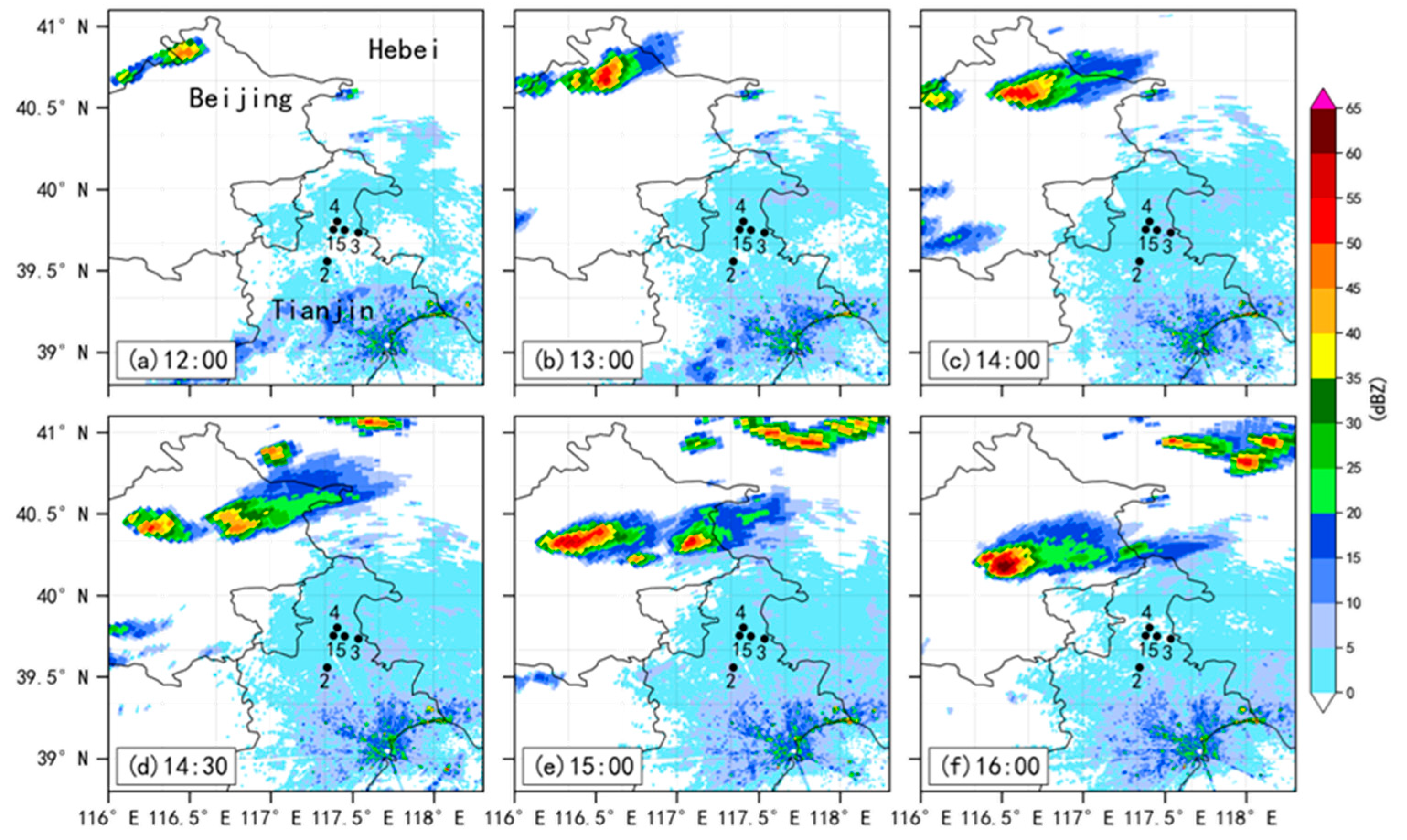
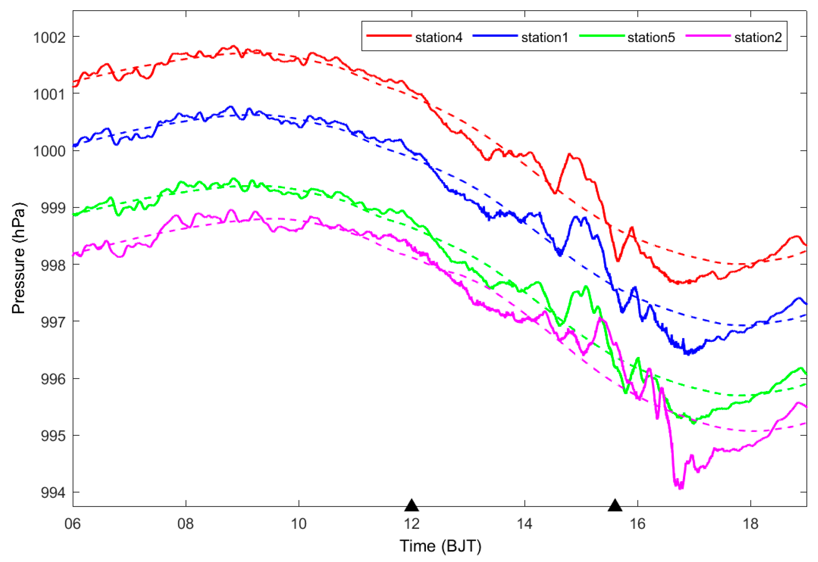
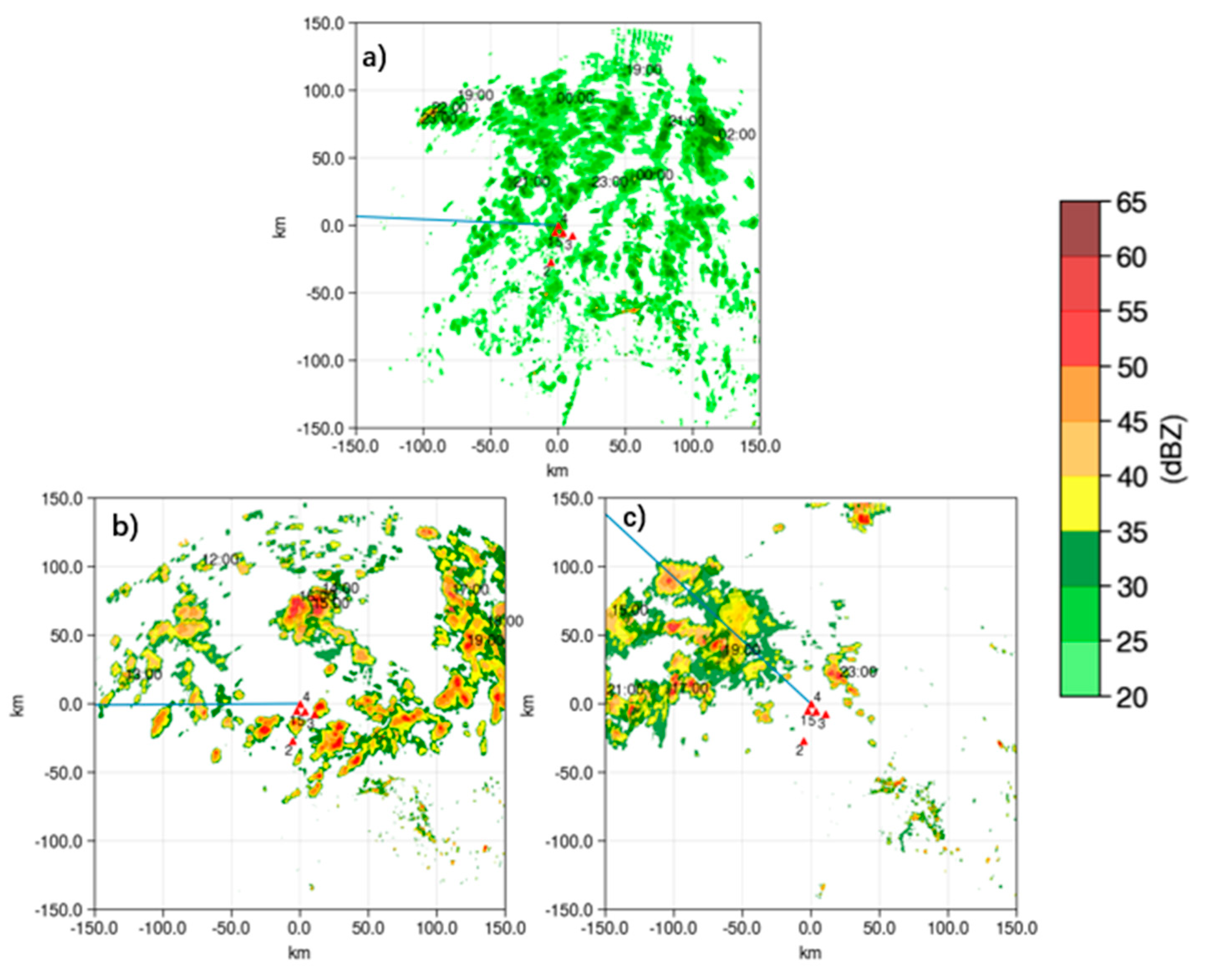
3.1. Convective Process

On 26 June 2018, medium-β-scale downhill convection in Beijing occurred from 12:00 (BJT, the same as below) to 17:00, with a maximum echo strength of 65 dBZ. As shown in Figure 1, this convective process had two successive convective clouds going downhill, and a convective process with an intensity of about 50 dBZ appeared in the mountainous area of northwestern Beijing at 12:00, and it gradually weakened and dispersed after moving downhill to the south. Around 12:42, a second convective process was triggered in the Yanqing area, moving southward, and convection was enhanced after the downhill movement. Around 13:00, a new convective process entered the radar observation range on the northeast side of Beijing, with an intensity of 50 dBZ, and the former reached 65 dBZ at 14:36, both of which gradually moved to the southeast direction and finally dissipated in around 17:00.

3.2. Gravity Wave Spectral Characteristics

Although the two convective clouds did not pass through the microbarographs during this process, significant barometric pressure fluctuations were observed at both sites. Figure 2 shows the raw data of the observation, and the trend shows the existence of a background field of daily barometric pressure variations; the peak is reached at around 9:00 and then a trough around 17:00, with a difference of about 430 Pa. At the same time, there is also a small fluctuating noise of the observations in the background field. When the convective cloud is triggered at 12:00, the air pressure first decreases and then rises, probably due to the influence of the updraft on the front side of the convection, and when the convective cloud gradually moves toward the stations, the accompanying downdraft arrives at the ground, which may result in the rise of the air pressure. Using low-pass filtering to filter out the fluctuations with a period larger than 8 h to obtain the disturbed air pressure, as shown in Figure 3, with the convective cloud close to the station, the amplitude of the air pressure gradually increases; the fluctuation signals of the four stations in this period of time are very similar, which can be considered to be caused by the same convection, and if we consider that the fluctuation is similar to a sinusoidal wave, and the oscillation of an upward one and a downward one is taken as a fluctuation, then the maximum amplitudes of stations four, one, five, and two correspond to 139.8, 128.3, 146.5, and 104.6 Pa. Since the convective cloud moves from northwest to south relative to the microbarograph network, the peak of fluctuation is first reached at about 14:57 at station four, followed by 15:04, 15:05, and 15:19 at stations one, five, and two, respectively; the difference in time between the stations facilitates the estimation of the fluctuation propagation characteristics, such as the speed of the gravity wave and azimuthal angle (Section 3.3).
Through the signal standardization, the power spectrum is obtained using the Fourier transform method, and the spectral characteristics of the signals at the four stations are more consistent, as shown in Figure 4; the dominant fluctuation cycle centers are at 195 min, 71 min, respectively, indicating that there is a long period and a short period acting together in the period, and the average frequency in the process is about 1.543 × 10⁻⁴ Hz using the power spectrum as the weights. For the study of the local gravity wave feature changes accompanying the convective process, the Morlet wavelet transform method is applied to the perturbed pressure after normalization. Figure 5 and Figure 6 are the corresponding wavelet real part spectra and power spectra at stations four, one, five, and two, which reflect the multi-scale features of the signals.
Taking station four as an example (Figure 5a), the long period fluctuations around 8:00 are mainly concentrated at around 200 min; there may be gravity wave precursor activity before the convective emergence, and the barometric pressure signal with a short period scale of about 70 min is very obvious in the period from 12:30 to 17:30. During this time, a convective formation and movement processes existed; as the convective cloud moved southward and gradually approached the microbarographs, smaller fluctuations with a time scale of 32 min appeared, and the convective cloud was the closest to the network at 15:36, with a strength of 45 dBZ, at which time the short-period fluctuations with a time scale of 20 min appeared but were maintained for half an hour only, and then, as the convective currents gradually weakened, the short-period fluctuations disappeared as the convection gradually weakened and moved away from the network. The remaining stations have similar fluctuation characteristics, but there are differences in the time of occurrence of the significant fluctuations, which are related to the sequence of the fluctuations arriving at the observing stations. Through the above Fourier transform method and wavelet analysis, the fluctuation characteristics related to convection are mainly divided into three frequency bands. We obtained that there may be precursor activity of the long−period gravity wave 4 h before convective triggering, with the main period range of about 140–250 min, while in the convective process, it is accompanied by multi-scale fluctuation interactions with the main period range of 45–105 min, and when the convective cloud is close to the station, there are fluctuations with shorter periods of about 16–30 min.
Since the emergence time of short-period fluctuations corresponds to the convective process, the wavelet power spectrum of short-period fluctuations (Figure 6) is able to show the most significant time scales in the fluctuations [56]. As shown in Figure 6, after the convection is triggered, the observed fluctuation signals are not obvious due to the distance from the observation station; the main period is concentrated at about 90 min when the convection gradually strengthens after descending down the mountain, the high-energy fluctuation signals are developed to the high-frequency, and the period of the high-power spectral fluctuation signals is about 23–96 min. When the convective cloud is close to the station, the fluctuation energy increases, and then, as the convection is weakened and gradually moves away from the station, the fluctuation is dissipated. The wavelet power spectrum is time-averaged over the period to obtain the global wavelet spectrum to be able to identify the characteristics of the periodic fluctuations and their intensities (Figure 7). According to the global spectrum of wavelet (Figure 7), station two is farther away from the convection, and gravity waves will be dissipated during the propagation process; thus, the curve is obviously weakened with respect to the other stations, and the main period range is shorter. Nevertheless, the period of the signals received by the four stations through the test is still in the range of 48–115 min, which indicates that the convective process is accompanied by the enhancement of the fluctuation energy, and there is a mixing of multiple-frequency fluctuations.

3.3. Characteristics of Gravity Wave Propagation

According to the above analysis, the main fluctuation period accompanying the convection is concentrated in 40–120 min, so using the filtering characteristics of wavelet analysis, the fluctuation within the period is reconstructed; as shown in Figure 8, the barometric fluctuation is stronger in the process of convection occurring from 12:00–18:00, the signal similarity is higher at each station, and there is a significant time delay between the peaks, but due to the fact that station two is far away from the other stations, the fluctuation deformation occurs, and the relevance to the other signals is weakened, therefore, in the calculation of fluctuation propagation characteristics, only stations one, four, and five are taken into account.
According to the above method, the wave velocity vector is calculated for the fluctuation signals from 12:00 to 18:00, and the correlation of the signals between stations four, one, and five is above 95%, which indicates that the observed signals are indeed caused by the same event, and the time delays between the two stations at the time of the maximum corresponding correlation are t14 = 352 s, t54 = 439 s, and t51 = 84 s, respectively, the wave velocity is about 14 m/s, and the azimuth angle is 95°. Using the obtained wave speeds to calculate the time delays of different grid points relative to each station and the measured time delays for the variance, when the value is taken as the minimum to obtain the approximate position of the wave source at (−14, 145) km (Figure 9b), the two convective cloud trigger positions during this period are about (−77, 116) km and (17, 141) km relative to the origin, and the estimation errors are 69.4 km and 31.3 km, respectively.
For the convective cloud moving southward from the northwest side of the station during the analyzed time, its orientation is more consistent with the fluctuation azimuth but with a slight deviation (Figure 9a), it is considered that the fluctuation is the gravity wave stimulated by convection, the deviation is considered to be due to the fact that two strong convections moved southward from the north-northwest side of the station successively in that period, the fluctuations accompanying them are superimposed on each other and cannot be differentiated by the relatively small number of observing stations, which results in estimation deviation, and the position of the wave source obtained from the calculation of the time-delay method can only roughly express the convective position, which is not able to be corresponded to the position of convection, so the method still needs to be improved.

4. Gravity Wave Characteristics of Multiple Convective Cases

By analyzing the fluctuation signal on 26 June 2018, the fluctuation amplitude is about 140 Pa at maximum, and the fluctuation period has two peaks of 195 min and 71 min, with an average frequency of about 1.543 × 10⁻⁴ Hz. Before the emergence of convective clouds, there is a long period of fluctuation of about 200 min; when the convective cloud is close to the microbarograph station, the fluctuation intensity is larger, and the fluctuation frequency is widened. Different frequency fluctuations work together in the convective process, and the fluctuation characteristics are mainly concentrated in three frequency bands: 16–30 min, 45–105 min, and 140–250 min. Through wavelet power analysis of the fluctuation signal, it is considered that the short period of fluctuation of this convection process is mainly concentrated in 48–115 min. The geometric relationship calculates that the wave speed in this frequency band is about 14 m/s, and the azimuth angle is about 95°, which is about the same as that of the convective cloud. The wave source location of (−14, 145) km is obtained from the time delay calculation, and the distance error from the convective cloud trigger location is roughly 69.4 km and 31.3 km.
According to the above method to analyze the remaining three cases, the fluctuation characteristics accompanying the convective process in different directions and with different intensities are counted, as shown in Table 1, the weaker intensity of convection on 22 June 2018, was only 40 dBZ, the maximum amplitude of fluctuation observed by the microbarographs was 65 Pa, the fluctuation frequency was still present with two peaks of 0.654 × 10⁻⁴ and 2.124 × 10⁻⁴ Hz, and the average frequency was about 1.632 × 10⁻⁴ Hz. Due to the convective intensity being weak, the gravity wave is not strong; through the wavelet analysis of the convective process, the accompanying fluctuation period is mainly concentrated in two bands, 43–100 min and 140–250 min, and the precursor activity occurs in advance of the convective trigger 4 h. The period range accompanying the convective process through wavelet power analysis is small, about 46–104 min, and the fluctuation speed in this frequency band is 14.6 m/s. Similarly, for the two convective processes on 29–30 June and 2018, their intensity reaches 60 dBZ, and the strongest barometric amplitudes observed are 168 and 144 Pa, which are similar to the previous studies [57]. The spectral analysis of the observed data shows that the short-period fluctuation energy is enhanced but still dominated by the long-period fluctuation, and the average frequencies are 1.57 × 10⁻⁴ Hz and 1.473 × 10⁻⁴ Hz, respectively. The obvious fluctuation characteristics are also mainly concentrated in three parts: 17–40 min, 45–115 min, and 125–250 min; 17–45 min, 55–115 min, and 130–250 min. For the long period of fluctuation, there is a precursor activity in advance of about 1–4 h, and through the wavelet power spectrum analysis, the peak values of the short-period fluctuation are concentrated in the 40–120 min, and the wave velocities of the two strong convective processes are calculated as 37 m/s and 17 m/s, respectively.
The above three convective processes are shown in Figure 10. On 22 June 2018, the cloud range was larger, but the convective intensity was weaker; only sporadic convective centers appeared in the clouds, moving eastward from the northwest side of the station; a weaker cloud band was formed at 22:00 and kept moving eastward; at 23:00 the cloud band passed over the station at this time, the observed pressure reached the peak of the maximum amplitude of about 65 Pa, and the estimated fluctuations in azimuth angle was about 177° (Figure 10a), due to the weak convective intensity and observation of strong fluctuations in a relatively short period, resulting in azimuthal estimation error. The location of the wave source is calculated to be (−141, 4) km by the method of minimizing the variance of the time delay, and the error with the location of the convective cloud emergence is large at 110.8 km (Figure 11a); On 29 June, 12:00 northwest of Beijing appeared convective clouds moving southeastward with a strength of 45 dBZ, followed by a strong convective cloud near Xinglong at about 13:40, which rapidly triggered enhanced southward movement with a strength of 60 dBZ, and at the same time, there was also a strong convective cloud on the northeast side of the station, moving in a southeasterly direction with a strength of 55 dBZ. Three convective clouds around 18:50 in the station southeast merged to form a strong convective cloud band gradually moving southeast; the process of the maximum amplitude of the pressure is about 168 Pa, and the estimated fluctuations in azimuth of about 180°. Due to the dispersed convective clouds and large intensity, the microbarograph network can only roughly estimate the convective clouds orientation and obtain the position of the wave source as (−150, 4) km, with an error of 88 km from the position of the convective flow (Figure 11b). On 30 June, convective clouds appeared near Yanqing at 15:00; moving eastward, two convective clouds merged, and the strength reached 60 dBZ at 18:30, and at 20:30, new convective clouds triggered downhill weakening, which led to the process of a pressure amplitude maximum of 144 Pa, fluctuations in azimuth of 137°, which is consistent with convective cloud orientation (Figure 10c). The calculated location of the wave source is (−150, 132) km, and the error between the location and the appearance of the convection is 67.1 km (Figure 11c).
Since the convective process is accompanied by a gravity wave, the main spectral characteristics of the fluctuations can be roughly obtained by microbarograph observation, and the short-period wave associated with convection is mainly concentrated at 40–120 min; the propagation characteristics of the fluctuations can be estimated to be about 14–37 m/s by using multiple microbarographs to form arrays, and the azimuthal position of the source can be roughly estimated by the geometric method and the calculation of the minimum of the variance of the time delay. However, the azimuthal estimation will have errors if the strong convection is more dispersed or the intensity is weaker; this is related to the deployment of the microbarograph arrays. Multiple array combinations may provide new ideas for convective cloud tracking.

5. Conclusions

In this paper, the wavelet transform was used to analyze the baroclinic pressure changes in four downhill convective processes occurring in the Beijing–Tianjin–Hebei region in June 2018. The comprehensive analysis of the real part of wavelet coefficients and the power spectrum of the observed signals shows that the air pressure change in the convective process has obvious multi-scale characteristics, and the up and down oscillation of the air pressure is often used to represent the amplitude change in fluctuation, so the analysis of the air pressure can obtain the characteristics of the convective flow accompanied by the fluctuation change as follows:
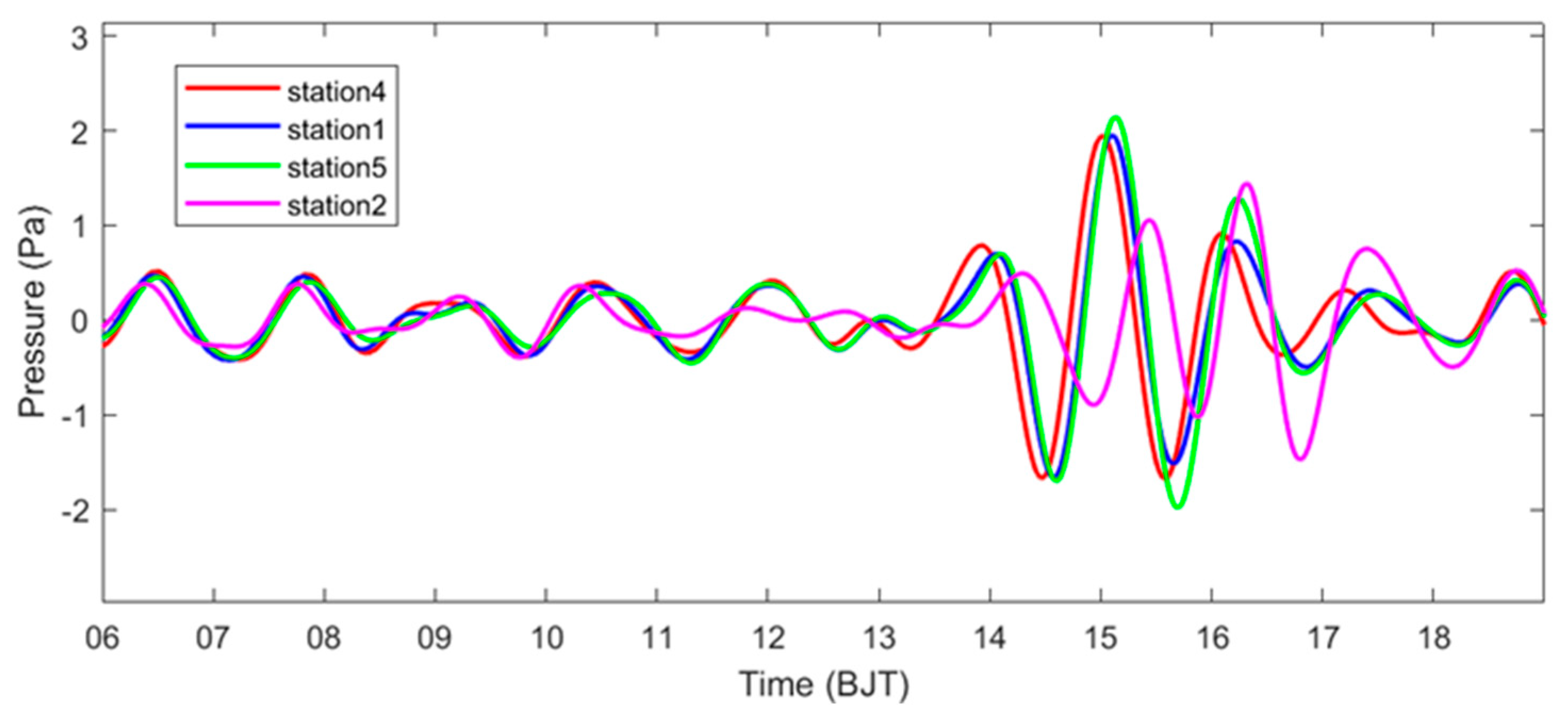
  • Multiple micromanometers observe the same convective process, and the accompanying fluctuation signals have a high degree of similarity. The stronger the convection, the larger the amplitude of the barometric pressure observed at the station, and the longer the strong fluctuations appear.
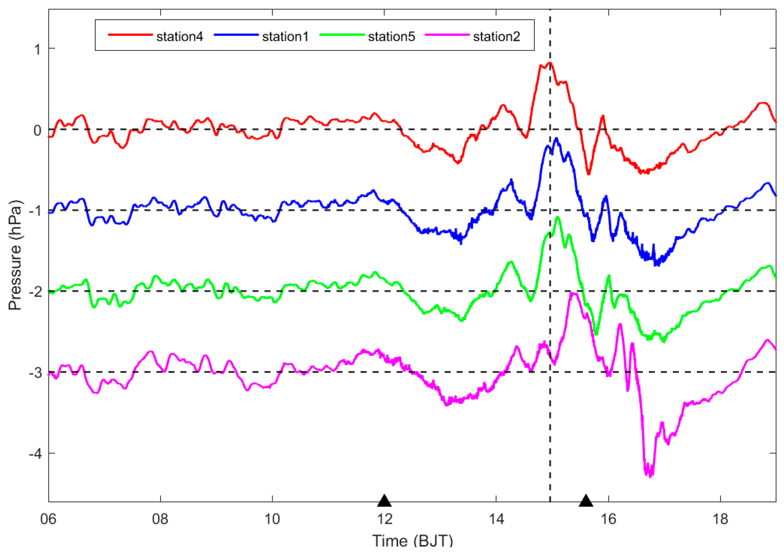
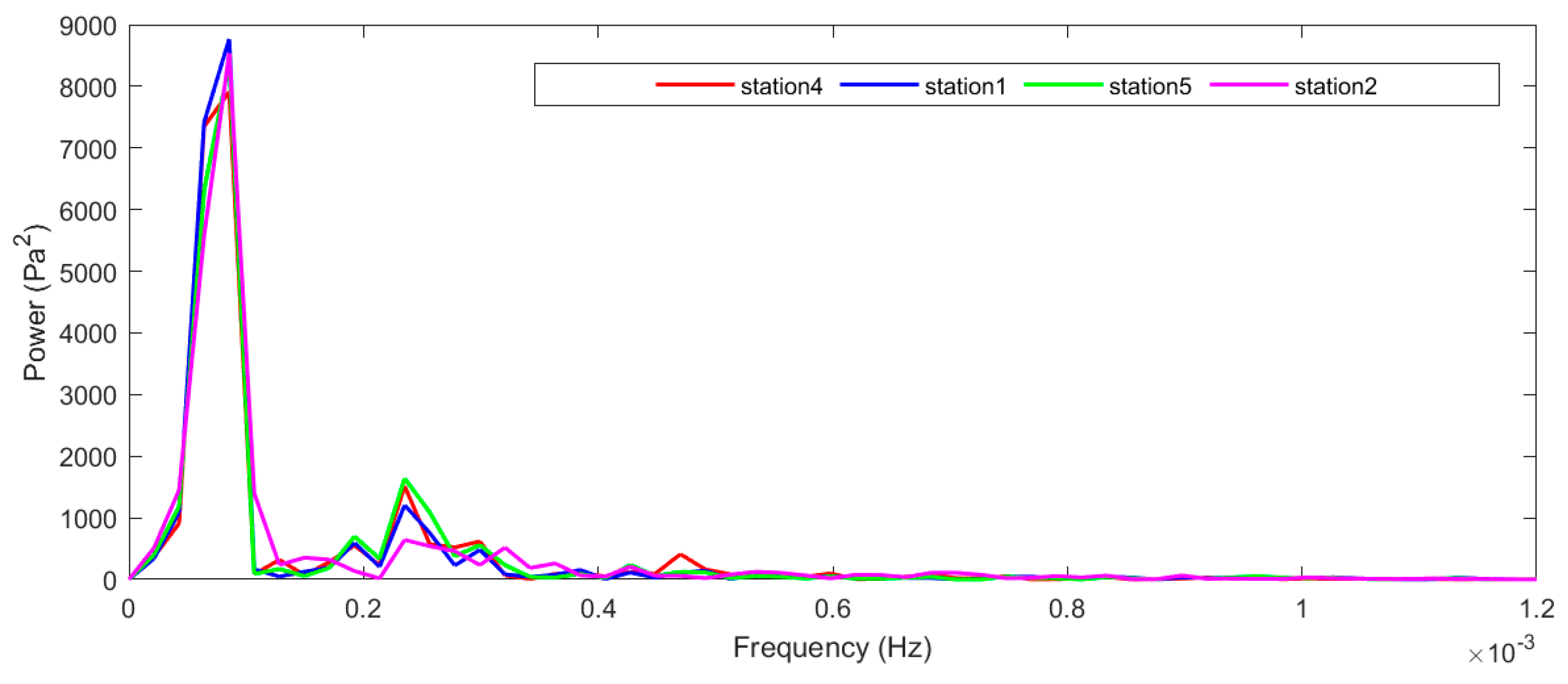
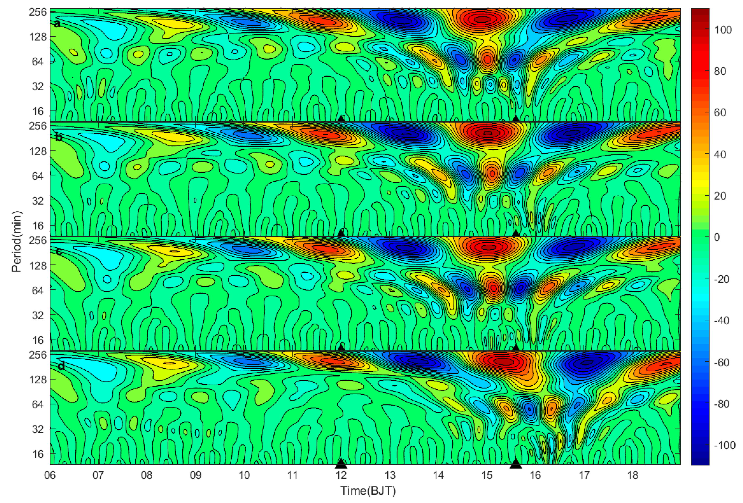
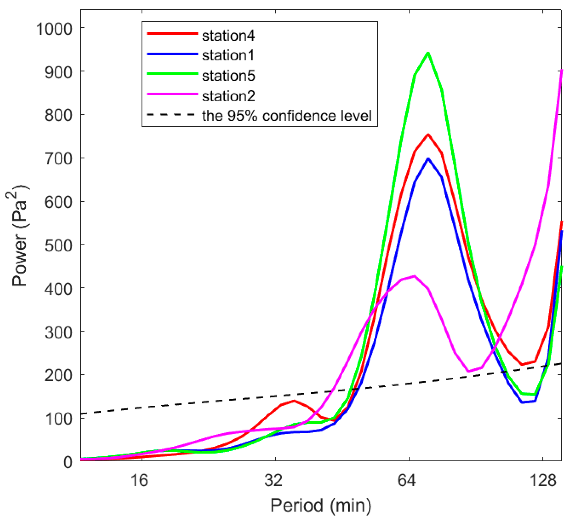
  • There are multi-scale spectral characteristics of the fluctuation process. Using Fourier analysis, the fluctuation of the long period was concentrated at 0.903 × 10⁻⁴ Hz, and the short period was concentrated at 2.04 × 10⁻⁴ Hz; wavelet analysis of the fluctuations found that the strong convection gravity wave period was mainly divided into three bands: 15–40 min, 40–120 min, 120–250 min; the longer period of fluctuations was in advance of the convection, which roughly appeared for 1–4 h, and the time of the short-period fluctuation was more consistent with the convective process. The period of the fluctuation was mostly concentrated at 40–120 min, and the fluctuation frequency broadened when convection was closer to the station. When the convection gradually closed toward the station, the fluctuation frequency broadened, which stimulated a smaller cycle of fluctuations. This conclusion is more consistent with previous studies [58,59,60]. The reconstruction of the 40–120 min period wave shows that the fluctuation characteristics were clearer, and the fluctuation reached its maximum amplitude before the convection was closest to the station and then gradually decreased, which was probably due to the unstable or weakly stable convective environment that can cause the dissipation of the gravity waves in the boundary layer [46].
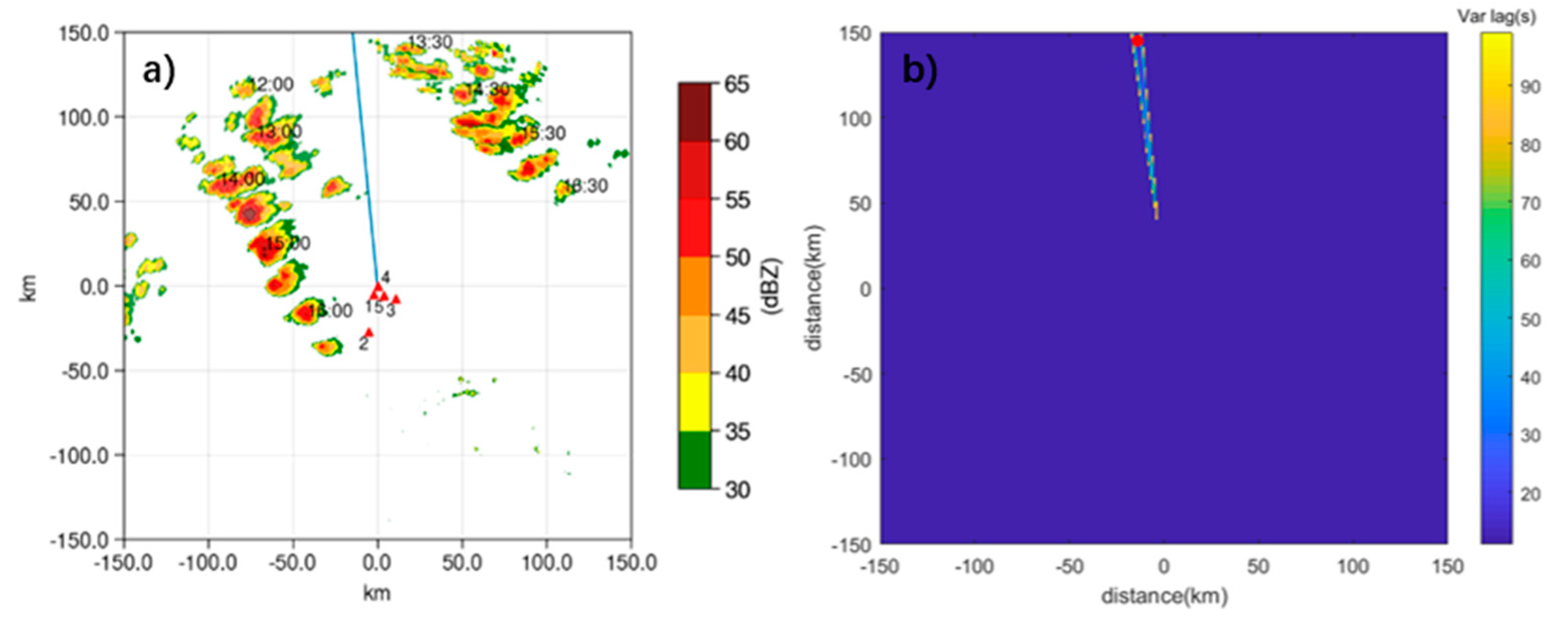
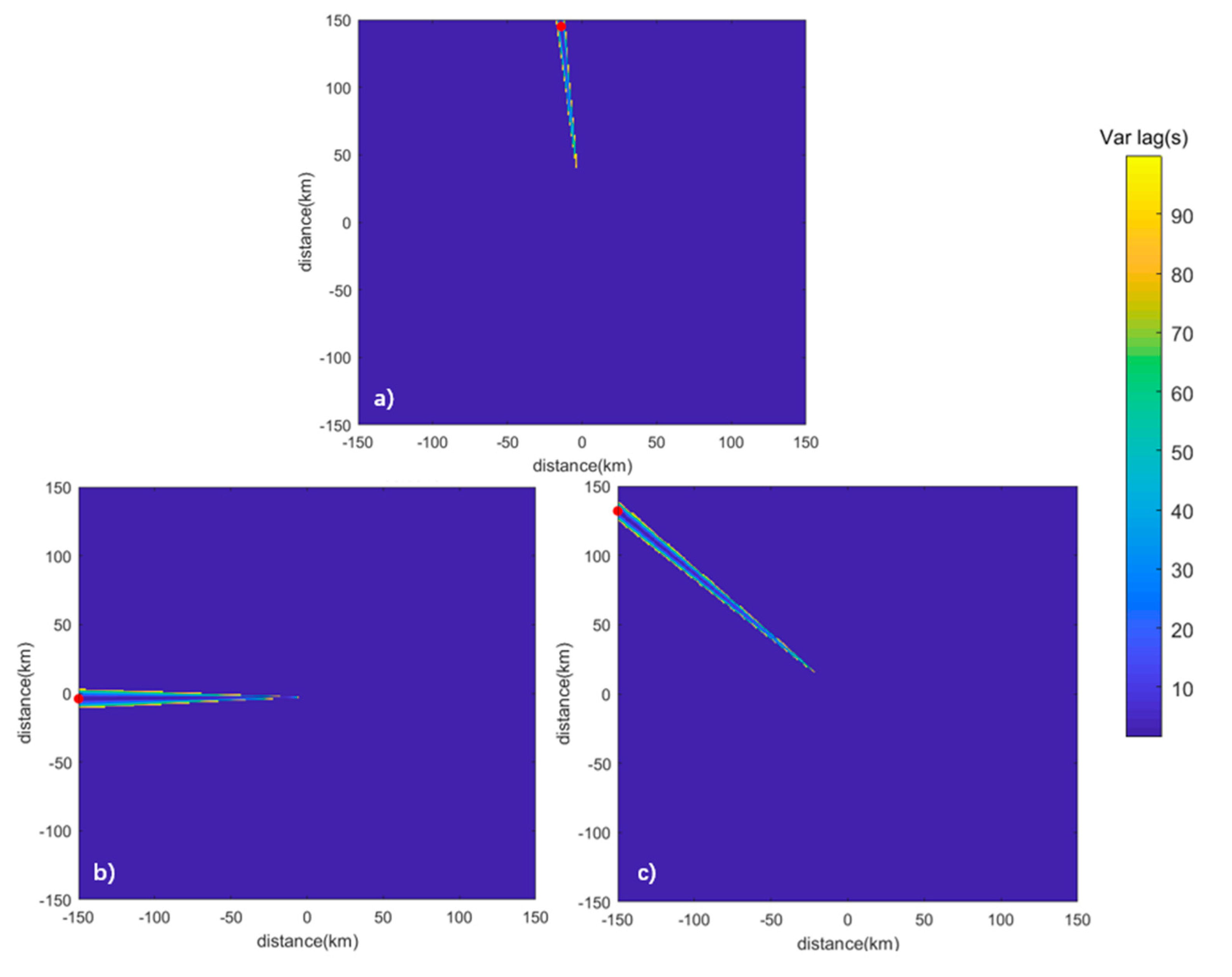
  • The fluctuation propagation characteristics were calculated for the 40–120 min reconstructed signals at stations four, one, and five; the wave speeds during convection were obtained as 14 m/s, 17 m/s, and 37 m/s, respectively, and the azimuthal angles of the wave sources were more consistent with the convective azimuths, but there were still deviations. Generally, the horizontal wave speed of inertial gravity waves ranged from about 10–50 m/s and often occurred in conjunction with convection [48,50,61], with a feedback mechanism between the two. The method of time-delay estimation could roughly estimate the position of the wave source, but the deviation was large, and the localization method still needs to be improved.
The above results show that convective processes are accompanied by gravity fluctuations on different time scales, and there is a precursor activity of long-period fluctuations before convection occurs. Similar phenomena have been analyzed by numerical simulations or meteorological station observations [51,62], but due to the lack of temporal resolution, it is not possible to analyze the characteristics of fluctuations over a shorter period, which can be compensated for by the observation of microbarographs. The use of microbarograph observations can better analyze the spectral and propagation characteristics of the short-period fluctuations. However, due to the existence of multi-frequency gravity waves in the convection process, it is necessary to study the fluctuation signals of different frequencies. In addition, the calculation of fluctuation characteristics is closely related to the deployment of stations, and more observation stations and reasonable deployment structures are conducive to a more accurate determination of the wave source. Therefore, the next step is to consider segmenting the fluctuation signals, analyzing the fluctuation characteristics of the signals in different frequency bands, and determining whether it is possible to utilize the observation of microbarographs to achieve the localization of the source of the wave.

Author Contributions

Methodology, H.L. and L.R.; Software, K.Z.; Writing—original draft, Y.L. All authors have read and agreed to the published version of the manuscript.

Funding

This research was funded by the Beijing Municipal Science and Technology Commission (Grant No. Z221100005222012), the Department of Science and Technology of Hebei Province (Grant No. 22375404D), the Open subjects of the Key Open Laboratory of Cloud Physical Environment, China Meteorological Administration (Grant No. 2020Z00715) and the National Natural Science Foundation of China (Grant Nos. U2233218 and 42275010).

Data Availability Statement

Not applicable.

Conflicts of Interest

The authors declare no conflict of interest.

References

  1. Hines, C.O. The upper atmosphere in motion. Q. J. R. Meteorol. Soc. 1963, 89, 1–42. [Google Scholar] [CrossRef]
  2. James, L. Waves in Fluids. Meas. Sci. Technol. 2002, 13, 1501. [Google Scholar]
  3. Carmen, J.N. Observations and Measurements of Gravity Waves. In An Introduction to Atmospheric Gravity Waves; Carmen, J.N., Ed.; Academic Press: Cambridge, MA, USA, 2012; Volume 102, pp. 231–278. [Google Scholar]
  4. Liu, L.; Ran, L.; Gao, S. Analysis of the Characteristics of Inertia-Gravity Waves during an Orographic Precipitation Event. Adv. Atmos. Sci. 2018, 35, 604–620. [Google Scholar] [CrossRef]
  5. Moffat-Griffin, T. An Introduction to Atmospheric Gravity Wave Science in the Polar Regions and First Results from ANGWIN. J. Geophys. Res. Atmos. 2019, 124, 1198–1199. [Google Scholar] [CrossRef]
  6. Rees, J.M.; Denholm-Price, J.C.W.; King, J.C.; Anderson, P.S. A Climatological Study of Internal Gravity Waves in the Atmospheric Boundary Layer Overlying the Brunt Ice Shelf, Antarctica. J. Atmos. Sci. 2000, 57, 511–526. [Google Scholar] [CrossRef]
  7. Jacques, A.A.; Horel, J.D.; Crosman, E.T.; Vernon, F.L. Tracking Mesoscale Pressure Perturbations Using the USArray Transportable Array. Mon. Weather Rev. 2017, 145, 3119–3142. [Google Scholar] [CrossRef]
  8. Hoffmann, L.; Alexander, M.J. Occurrence frequency of convective gravity waves during the North American thunderstorm season. J. Geophys. Res. Atmos. 2010, 115, D20111. [Google Scholar] [CrossRef]
  9. de Groot-Hedlin, C.D.; Hedlin, M.A.H.; Hoffmann, L.; Alexander, M.J.; Stephan, C.C. Relationships between Gravity Waves Observed at Earth’s Surface and in the Stratosphere Over the Central and Eastern United States. J. Geophys. Res. Atmos. 2017, 122, 11482–11498. [Google Scholar] [CrossRef]
  10. Holton, J.R. The Influence of Gravity Wave Breaking on the General Circulation of the Middle Atmosphere. J. Atmos. Sci. 1983, 40, 2497–2507. [Google Scholar] [CrossRef]
  11. Kim, Y.J.; Eckermann, S.D.; Chun, H.Y. An overview of the past, present and future of gravity-wave drag parametrization for numerical climate and weather prediction models. Atmos. Ocean 2003, 41, 65–98. [Google Scholar]
  12. Lindzen, R.S. Turbulence and stress owing to gravity wave and tidal breakdown. J. Geophys. Res. Ocean 1981, 86, 9707–9714. [Google Scholar] [CrossRef]
  13. Vincent, R.A.; Reid, I.M. HF Doppler Measurements of Mesospheric Gravity Wave Momentum Fluxes. J. Atmos. Sci. 1983, 40, 1321–1333. [Google Scholar] [CrossRef]
  14. Holton, J.R. The Role of Gravity Wave Induced Drag and Diffusion in the Momentum Budget of the Mesosphere. J. Atmos. Sci. 1982, 39, 791–799. [Google Scholar] [CrossRef]
  15. Fritts, D.C.; Alexander, M.J. Gravity wave dynamics and effects in the middle atmosphere. Rev. Geophys. 2003, 41, 1003. [Google Scholar] [CrossRef]
  16. Lane, T.P.; Zhang, F. Coupling between Gravity Waves and Tropical Convection at Mesoscales. J. Atmos. Sci. 2011, 68, 2582–2598. [Google Scholar] [CrossRef]
  17. Schmidt, J.M.; Cotton, W.R. Interactions between upper and lower tropospheric gravity waves on squall line structure and maintenance. J. Atmos. Sci. 1990, 47, 1205–1222. [Google Scholar] [CrossRef]
  18. Pandya, R.E.; Durran, D.R.; Weisman, M.L. The influence of convective thermal forcing on the three-dimensional circulation around squall lines. J. Atmos. Sci. 2000, 57, 29–45. [Google Scholar] [CrossRef]
  19. Liu, C.; Moncrieff, M.W. Effects of Convectively Generated Gravity Waves and Rotation on the Organization of Convection. J. Atmos. Sci. 2004, 61, 2218–2227. [Google Scholar] [CrossRef]
  20. Uccelini, L.W. A Case Study of Apparent Gravity Wave Initiation of Severe Convective Storms. Mon. Weather Rev. 1975, 103, 497–513. [Google Scholar] [CrossRef]
  21. Lindzen, R.S. Wave-CISK in the Tropics. J. Atmos. Sci. 1974, 31, 156–179. [Google Scholar] [CrossRef]
  22. Raymond, D.J. A Model for Predicting the Movement of Continuously Propagating Convective Storms. J. Atmos. Sci. 1975, 32, 1308–1317. [Google Scholar] [CrossRef]
  23. Gong, D.; Wu, Z.; Fu, G. Analysis of the Mesoscale Characteristics About a Severe Thunderstorm in North China. Chin. J. Atmos. Sci. 2005, 29, 453–464. [Google Scholar]
  24. Xie, J.; Li, G. Mechanism Analysis of a Sudden Rainstorm Triggered by the Coupling of Gravity Wave and Convection in Mountainous Area. Chin. J. Atmos. Sci. 2021, 45, 617–632. [Google Scholar]
  25. Huang, X.; Zhou, Y.; Liu, L. Occurrence and Development of an Extreme Precipitation Event in the Ili Valley, Xinjiang, China and Analysis of Gravity Waves. Atmosphere 2020, 11, 752. [Google Scholar] [CrossRef]
  26. Su, T.; Zhai, G. The Role of Convectively Generated Gravity Waves on Convective Initiation: A Case Study. Mon. Weather Rev. 2017, 145, 335–359. [Google Scholar] [CrossRef]
  27. Li, M. Studies on the gravity wave initiation of the excessively heavy rainfall. Chin. J. Atmos. Sci. 1978, 2, 201–209. [Google Scholar]
  28. Sun, Y.; Li, Z.; Shou, S. A mesoscale analysis of the snowstorm event of 3-5 March 2007 in Liaoning Province. Acta Meteorol. Sin. 2012, 70, 936–948. [Google Scholar]
  29. Ma, S.; Ran, L.; Cao, J.; Jiao, B.; Zhou, K. Characteristics for the sources and sinks of gravity waves in an orographic heavy snowfall event. Front. Earth Sci. 2023, 17, 604–619. [Google Scholar] [CrossRef]
  30. Zhang, Y.; Xiong, J.; Wan, W. Analysis on the Global Morphology of Middle Atmospheric Gravity Waves. Chin. J. Geophys. 2011, 54, 427–435. [Google Scholar] [CrossRef]
  31. Murphy, D.J.; Alexander, S.P.; Klekociuk, A.R.; Love, P.T.; Vincent, R.A. Radiosonde observations of gravity waves in the lower stratosphere over Davis, Antarctica. J. Geophys. Res. Atmos. 2014, 119, 11,973–11,996. [Google Scholar] [CrossRef]
  32. Yao, Z.; Hong, J.; Han, Z.; Zhao, Z. Numerical Simulation of Typhoon-generated Gravity Waves Observed by Satellite and its Direct Validationormalsize. Chin. J. Space Sci. 2018, 38, 188–200. [Google Scholar]
  33. Zhang, N.; Zhao, R.; Sun, D.; Han, Y.; Chen, C. Inertial gravity waves study with Rayleigh Doppler Lidar long-term observation. Infrared Laser Eng. 2020, 49, 20200351. [Google Scholar]
  34. Yang, C.; Guo, Q.; Cao, X.; Zhang, W. Analysis of gravity wave characteristics in the lower stratosphere based on new round-trip radiosonde. Acta Meteorol. Sin. 2021, 79, 150–167. [Google Scholar]
  35. Brunk, I.W. The Pressure Pulsation of 11 April 1944. J. Atmos. Sci. 1949, 6, 181–187. [Google Scholar] [CrossRef]
  36. Bosart, L.F.; Cussen, J.P. Gravity Wave Phenomena Accompanying East Coast Cyclogenesis. Mon. Weather Rev. 1973, 101, 446–454. [Google Scholar] [CrossRef]
  37. Eom, J.K. Analysis of the Internal Gravity Wave Occurrence of 19 April 1970 in the Midwest. Mon. Weather Rev. 1975, 103, 217–226. [Google Scholar] [CrossRef]
  38. Donn, W.L.; Rind, D. Natural Infrasound as an Atmospheric Probe. Geophys. J. Int. 1971, 26, 111–133. [Google Scholar] [CrossRef]
  39. Curry, M.J.; Murty, R.C. Thunderstorm-Generated Gravity Waves. J. Atmos. Sci. 1974, 31, 1402–1408. [Google Scholar] [CrossRef]
  40. Whitaker, R.W.; Mutschlecner, J.P. A comparison of infrasound signals refracted from stratospheric and thermospheric altitudes. J. Geophys. Res. Atmos. 2008, 113, D08117. [Google Scholar] [CrossRef]
  41. Jacques, A.A.; Horel, J.D.; Crosman, E.T.; Vernon, F.L. Central and eastern U.S. surface pressure variations derived from the USArray network. Mon. Weather Rev. 2015, 143, 1472–1493. [Google Scholar] [CrossRef]
  42. Šindelárová, T.; Kozubek, M.; Chum, J.; Potužníková, K. Seasonal and diurnal variability of pressure fluctuation in the infrasound frequency range observed in the Czech microbarograph network. Stud. Geophys. Geod. 2016, 60, 747–762. [Google Scholar] [CrossRef]
  43. Keliher, T.E. The occurrence of microbarograph-detected gravity waves compared with the existence of dynamically unstable wind shear layers. J. Geophys. Res. 1975, 80, 2967–2976. [Google Scholar] [CrossRef]
  44. Smart, E.; Flinn, E.A. Fast Frequency-Wavenumber Analysis and Fisher Signal Detection in Real-Time Infrasonic Array Data Processing. Geophys. J. Int. 1971, 26, 279–284. [Google Scholar] [CrossRef]
  45. Denholm-Price, J.C.W.; Rees, J.M. Detecting Waves Using an Array of Sensors. Mon. Weather Rev. 1999, 127, 57–69. [Google Scholar] [CrossRef]
  46. Zhang, F.; Davis, C.A.; Kaplan, M.L.; Koch, S.E. Wavelet analysis and the governing dynamics of a large-amplitude mesoscale gravity-wave event along the East Coast of the United States. Q. J. R. Meteorol. Soc. 2001, 127, 2209–2245. [Google Scholar] [CrossRef]
  47. Chen, D.; Chen, Z.; Lü, D. Spatiotemporal spectrum and momentum flux of the stratospheric gravity waves generated by a typhoon. Sci. China Earth Sci. 2013, 56, 54–62. [Google Scholar] [CrossRef]
  48. Hauf, T.; Finke, U.; Neisser, J.; Bull, G.; Stangenberg, J.G. A Ground-Based Network for Atmospheric Pressure Fluctuations. J. Atmos. Ocean Technol. 1996, 13, 1001–1023. [Google Scholar] [CrossRef]
  49. Lu, C.; Koch, S.; Wang, N. Determination of temporal and spatial characteristics of atmospheric gravity waves combining cross-spectral analysis and wavelet transformation. J. Geophys. Res. Atmos. 2005, 110, D01109. [Google Scholar] [CrossRef]
  50. Li, Q.; Xie, J.; Yang, X. The Dynamic Characteristics of Gravity Waves during Severe Hailstorm Process. Acta Meteorol. Sin. 1993, 51, 361–368. [Google Scholar]
  51. Wu, L.; Wen, Z.; He, H. Relationship between the Periodic Fluctuations of Pressure and Precipitation during a Rainstorm. Atmos. Ocean Sci. Lett. 2015, 8, 78–81. [Google Scholar]
  52. Wang, X.; Lei, H.; Jiang, Z.; Zheng, S.; Qi, Y. Frequency Spectrum Dynamic Characteristics of Atmospheric Gravity Waves during Various Types of Thunderstorms in Foshan. Clim. Environ. Res. 2021, 26, 250–262. [Google Scholar]
  53. Torrence, C.; Webster, P.J. Interdecadal Changes in the ENSO–Monsoon System. J. Clim. 1999, 12, 2679–2690. [Google Scholar] [CrossRef]
  54. Torrence, C.; Compo, G.P. A Practical Guide to Wavelet Analysis. Bull. Am. Meteorol. Soc. 1998, 79, 61–78. [Google Scholar] [CrossRef]
  55. Yang, Q.; Ding, H.; Xia, Y. Source Location of Infrasonic by Tripartite Array Arithmetic. Beijing Gongye Daxue Xuebao/J. Beijing Univ. Technol. 2017, 43, 819–825. [Google Scholar]
  56. Melissa, J.L.; Martin, J.S. Wavelet analysis of inter-annual variability in the runoff regimes of glacial and nival stream catchments, Bow Lake, Alberta. Hydrol. Process. 2003, 17, 1093–1118. [Google Scholar]
  57. Koch, S.E.; Siedlarz, L.M. Mesoscale Gravity Waves and Their Environment in the Central United States during STORM-FEST. Mon. Weather Rev. 1999, 127, 2854–2879. [Google Scholar] [CrossRef]
  58. Wang, X.; Lei, H.; Feng, L.; Zhu, J.; Li, Z.; Jiang, Z. Analysis of the characteristics of gravity waves during a local rainstorm event in Foshan, China. Atmos. Ocean. Sci. Lett. 2020, 13, 163–170. [Google Scholar] [CrossRef]
  59. Wang, X.; Ran, L.; Qi, Y.; Ma, S.; Mu, X.; Jiang, Z.; Bi, X. Analysis of characteristics of gravity waves of heavy rainfall event based on microbarograph observation. Acta Phys. Sin. 2021, 70, 234702. [Google Scholar] [CrossRef]
  60. Wang, X.; Ran, L.; Qi, Y.; Jiang, Z.; Yun, T.; Jiao, B. Analysis of Gravity Wave Characteristics during a Hailstone Event in the Cold Vortex of Northeast China. Atmosphere 2023, 14, 412. [Google Scholar] [CrossRef]
  61. Blanc, E.; Farges, T.; Le Pichon, A.; Heinrich, P. Ten year observations of gravity waves from thunderstorms in western Africa. J. Geophys. Res. Atmos. 2014, 119, 6409–6418. [Google Scholar] [CrossRef]
  62. Yang, R.; Liu, Y.; Ran, L.; Zhang, Y. Simulation of a torrential rainstorm in Xinjiang and gravity wave analysis. Chin. Phys. B 2018, 27, 059201. [Google Scholar] [CrossRef]
Figure 1. 26 June 2018 12:00–16:00 (af) Tianjin Tanggu Measurement Station Radar Combined Reflectivity Factor (unit: dBZ); (a) 12:00, (b) 13:00, (c) 14:00, (d) 14:30, (e) 15:00, and (f) 16:00. The “•” in the figure are micromanometer stations 1–5.
Remotesensing 15 05024 g001
Figure 2. The original signal of barometric pressure (unit: hPa) was observed by microbarograph stations 4, 1, 5, and 2 at 6:00–19:00, the dotted line indicates the daily change signal of each station, in order to make a clear display, the interval between the signals is 1 hPa, the “▲” in the figure indicates the time of the emergence of convection at 12:00 and the closest to the station at 15:36 (the same below).
Remotesensing 15 05024 g002
Figure 3. Microbarograph stations 4, 1, 5, and 2 filter out barometric signals with a period greater than 8 h between 6:00 and 19:00 (uint: hPa), with an interval of 1 hPa between signals, the vertical dotted line indicates the time of the peak of the barometric pressure at station 4 at 15:19.
Remotesensing 15 05024 g003
Figure 4. Barometric power spectra observed at microbarograph stations 1, 2, 4, and 5 during 6:00−19:00 (unit: Pa2).
Remotesensing 15 05024 g004
Figure 5. Wavelet real part spectra of normalized barometric pressure observed at microbarograph stations 1, 2, 4, and 5 during 6:00−19:00; (a) station 4, (b) station 1, (c) station 5, and (d) station 2.
Remotesensing 15 05024 g005
Figure 6. Wavelet power spectra of the normalized barometric pressure observed at microbarograph stations 1, 2, 4, and 5 during 6:00–19:00; (a) station 4, (b) station 1, (c) station 5, and (d) station 2. The green line in the figure encloses the region with a confidence level of 95% or higher, and the shaded area is the wavelet influence cone.
Remotesensing 15 05024 g006
Figure 7. Wavelet global spectrum normalized to the observed pressure at microbarograph stations 1, 2, 4, and 5 during 6:00–19:00. The dashed line in the figure indicates a confidence level of 95% or higher.
Remotesensing 15 05024 g007
Figure 8. The reconstruction of the barometric data for a period of 40−120 min was observed by the microbarographs at stations 1, 2, 4 and 5 from 6:00 to 19:00.
Remotesensing 15 05024 g008
Figure 9. (a) Fluctuating azimuth estimates (b) wave source position estimation for the convective process on 26 June 2018, 12:00−17:00 (colored shading indicates convective cloud position over time, the blue line indicates the fluctuating azimuth estimate, rotated counterclockwise at 0° due east of station 4, and the “▲” indicates the position of the micropyrometer station; filled colors indicate time delay variance, “•” indicates the estimated position of the wave source).
Remotesensing 15 05024 g009
Figure 10. Three convective processes on June 2018, (a) 22, (b) 29, and (c) 30, and fluctuating azimuth estimates (colored shading indicates convective cloud position over time, the blue line indicates fluctuating azimuth estimate, rotated counterclockwise at 0° due east of station 4 to obtain azimuths of 177°, 180°, and 137°, respectively).
Remotesensing 15 05024 g010
Figure 11. Estimated wave source locations for three convective processes on June (a) 22, (b) 29, and (c) 30, 2018 (colored shading indicates the variance of time−delay estimates, “•” indicates estimated wave source location).
Remotesensing 15 05024 g011
Table 1. Gravity wave characterization statistics for four convective cases.
22 June 201826 June 201829 June 201830 June 2018
Time of convection emergence18:0012:0012:0015:00
Moment when convection is closest to the stations23:0015:3618:0022:00
Maximum combined reflectivity (dBZ)40656060
Maximum amplitude of air pressure (Pa)65139.8167.6144
Average frequency (10−4 Hz)1.6321.5431.5701.473
Short period range (min)46.6–103.548.3–114.853.6–110.946.6–110.9
Wave velocity
(m/s)
14.614.136.917.6
Wave azimuth
(°)
177.595.6180.4137.3
Wave source
location (km)
(−141,4)(−14,145)(−150,4)(−150,132)
Estimation error (km)110.869.4, 31.38867.1
Disclaimer/Publisher’s Note: The statements, opinions and data contained in all publications are solely those of the individual author(s) and contributor(s) and not of MDPI and/or the editor(s). MDPI and/or the editor(s) disclaim responsibility for any injury to people or property resulting from any ideas, methods, instructions or products referred to in the content.

