Statistical Analysis of High–Energy Particle Perturbations in the Radiation Belts Related to Strong Earthquakes Based on the CSES Observations

Lu Wang; Zhenxia Zhang; Zeren Zhima; Xuhui Shen; Wei Chu; Rui Yan; Feng Guo; Na Zhou; Huaran Chen; Daihui Wei

doi:10.3390/rs15205030

Abstract

Earthquakes (EQs) are a significant natural threat to humanity. In recent years, with advancements in space observation technology, it has been put forward that the electromagnetic effects of earthquakes can propagate into space in various ways, causing electromagnetic radiation and plasma disturbances in space and leading to high–energy particle precipitation. The China Seismo-Electromagnetic Satellite (CSES) is specifically designed for monitoring the space electromagnetic environment. In our study, we select 78 strong earthquakes from September 2018 to February 2023 (global earthquakes with M ⩾ 7.0 and the major seismic regions in China with M ⩾ 6.0). We focus on

10^{\circ}

of the latitude and longitude around the epicenter, spanning from 15 days before the earthquake to 5 days after, and look for anomalies in spatial evolution and temporal evolution. We present some typical cases of electron flux perturbation and summarize the anomalies of all 78 cases to look for regularity in EQ–related particle anomalies. Notably, we introduce two cases of simultaneous electromagnetic and energetic particle anomalies during earthquakes. And we propose a conjecture that the particle precipitation may be the result of wave–particle interactions triggered by seismic activity.

Keywords:

earthquakes; CSES; high–energy particle; wave–particle interaction

1. Introduction

Strong earthquakes (EQs) are one of the most destructive natural hazards, claiming countless deaths and economic losses. In recent years, with the development of satellite observations, new possibilities for earthquake prediction have arisen. Some space experiments have found that electromagnetic signals are observed during earthquakes, and these signals cover a wide range of phenomena, including electromagnetic wave interference, magnetic and electric field anomalies, and energetic particle precipitation. By studying these signals, scientists aim to unlock the potential for early earthquake detection and prediction [1,2,3,4].

It is necessary to mention a number of satellite experiments, the MARIYA, MARIYA-2, DEMETER, PET/SAMPEX, POES, ARINA, and CSES, which aim to study electron bursts and the geophysical effects causing them. In the late 1980s, Voronov S.A. analyzed the data of the MARIA experiment for the first time and reported the correlation between short-term energetic particle bursts in near-Earth space and the EQ activity [5]. Ruzhin Yu. Ya and Depueva, A.K. reported the simultaneous measurement of VLF electromagnetic wave and high–energy particle anomalies before the EQ in 1996 [6]. In addition, the most relevant work is that Aleksandrim found a concentration of particle bursts in the ionosphere 2–5 h before a major EQ through the statistical work of several satellites over nearly 20 years, which confirmed the correlation between particle bursts and seismic activity [2]. Based on the SAMPEC/PET satellite, Sgrigna also observed a significant increase in the number of energetic particles associated with EQs about 4 h before the EQ [7]. In the early 21st century, the DEMETER satellite was successfully launched by France and was in orbit from 2004 to 2010, which was the first space-monitoring satellite aimed at studying natural disasters such as EQs, volcanic eruptions, and ionospheric disturbances caused by human activities [8]. Some scholars also reported some work on the association of particle storm observations and EQs based on DEMETER satellite data [4,9,10,11]. There are also some important statistics works. Based on the NOAA satellites, the Fidani and Battiston statistics of the temporal distribution of EQ-related energetic particle anomalies showed correlation peaks found at −1.25 to +0.25 h before the EQ and 2–3 h before the EQ, respectively [12,13,14].

In recent years, some scholars made fresh explorations on the lithosphere–atmosphere–ionosphere coupling model and proposed possible hypotheses on the coupling mechanism of lithospheric activity and the ionosphere by the chemical path, acoustic path, and electromagnetic path [15,16,17,18]. During the propagation or onset of an EQ, the Earth’s inner lithosphere may emit electromagnetic radiation. This radiation can then propagate upward into the ionosphere, influencing the plasma parameters by impacting the processes of heating and ionization. In some cases, these electromagnetic waves also lead to the pitch–angle scattering of high–energy electrons through wave–particle interactions, resulting in particle precipitation [19,20]. Extensive research has accumulated a wealth of evidence regarding potential seismo-ionospheric precursor signatures. However, the precise mechanism by which EQ-induced ELF/VLF electromagnetic radiation affects the ionosphere and radiation belts and causes ionospheric perturbations and energetic particle precipitation remains unresolved [21,22,23,24,25].

The CSES is the first space–based platform in China for both EQ observation and geophysical field measurement. A space platform is established for monitoring global space electromagnetic waves/fields, ionospheric plasma, high–energy particles, and space weather. In recent years, the CSES team has analyzed the correlation of EQ–space electromagnetic disturbance phenomena around strong EQs (M ≥ 7.0 globally and M ≥ 6.0 in China) and obtained a great deal of research results [26,27,28,29,30]. For example, Zhima summarized data from multiple payloads of the satellite, observing a wide range of seismo–ionospheric perturbations, including electric fields, magnetic fields, TECs, etc. [31]. Zhu statistically examined the 2.5 years of Ne data from the CSES during the M ≥ 4.8 EQs worldwide. They found that significant positive Ne variations related to EQs mainly occurred 1 to 7 days and 13 to 15 days before the EQs [32].

The above studies and experiments confirm that the electromagnetic effects generated during EQs exist objectively. The study of EQ-induced spatial perturbations in the past has mainly focused on electromagnetic fields but not energetic particle precipitation. This paper counts 78 strong earthquakes from September 2018 to February 2023 based on the data of the CSES, including the global EQs with magnitude ⩾7.0, and the major seismic regions in China with magnitude ⩾6.0 (refer to the National Earthquake Science Data Sharing Center for the earthquake catalog). We analyze the energetic particle flux data within

\pm 10^{\circ}

longitude and latitude from the epicenter and count the data from 15 days before to 5 days after the quake. Finally, we perform a spatial and temporal analysis of the anomalies. And we summarize these anomalies to look for regularity in enhanced EQ–related particle flux.

2. Data Introduction and Analysis

On 2 February 2018, the CSES was launched into solar synchronous orbits with an altitude of 507 km and a

97^{\circ}

inclination. The orbit cycle is 94.6 min, and the ascending node is 14:00 p.m. with a revisiting period of 5 days. The CSES carries eight scientific payloads, of which the particle detector package consists of a high–energy band probe (HEPP–H), a low-energy band probe (HEPP–L), and a solar X–ray monitor (HEPP–X) [33,34]. HEPP–L is installed on the side of the satellite facing the Earth (YOZ) and has an angle of

20^{\circ}

with the Sun–Earth line. HEPP–L can measure the electron fluxes with an energy range from 0.1 MeV to 3 MeV. The energy ranges are divided into 256 energy channels with an energy resolution of ≥8.9% at 1 MeV for the electron. The maximum field of view of HEPP–L is

100^{\circ} \times 30^{\circ}

; it is composed of nine silicon slice detector units and the nine units are divided into two groups according to their field of view: five units with a narrow half angle of

6 . 5^{\circ}

and four units with a wide half angle of

15^{\circ}

. In our previous work, we have assessed the data quality of HEPP–L and it is accurate and valid [35].

The search coil magnetometer (SCM) onboard the CSES is designed to measure the magnetic field fluctuation of low-frequency electromagnetic waves in the frequency range of 10 Hz–20 kHz. The observed data of the 3 components of the SCM are divided by frequency bands, including 10–200 Hz (ULF), 200 Hz–2.2 kHz (ELF), and 1.8–20 kHz (VLF). The sampling rate of the SCM is 51.2 kHz and the time resolution of the power spectrum density (PSD) is 2 s. The frequency resolution is 12.5 Hz [36].

Data Selection and Data Preprocessing Methods

We only selected global earthquakes of magnitude ⩾7.0 all over the world and magnitude ⩾6.0 in the major EQ belts such as the Sichuan–Tibet and Taiwan EQ belts in Asia. For aftershocks that occurred within 5 days after the main EQ, we kept only the main EQ; a total of 78 EQs from September 2018 to February 2023 were counted in the statistics, as shown in Figure 1.

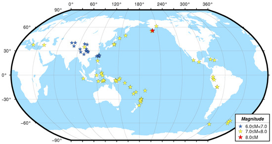
Figure 1. Global Distribution of 78 Earthquakes Observed by CSES from September 2018 to February 2023.

According to the formula for estimating the dimensions of the lithospheric pregnant seismic zone proposed by Dobrovolsky [37],

R = 10^{0.43 M}

(1)

R is the diameter of the gestation zone in km, and M is the magnitude of the EQ. This study primarily centers on EQ cases with magnitudes around 7.0, with only one exception exceeding magnitude 8. We determined the Dobrowolski radius of M 7.0 to be 1023 km, equivalent to a latitude/longitude span of approximately 10

^{\circ}

. Consequently, we employed 10

^{\circ}

as our search area to detect anomalies associated with EQs.

The perturbations of the solar and interplanetary magnetic fields on the ionosphere may mask the anomalous information generated by the EQs. We only focused on the anomalies under quiet space weather conditions to avoid the influence of complex space weather conditions. The Dst index (Disturbance Storm Time index) is a metric used to gauge the level of activity in Earth’s magnetic field. It is typically employed to characterize disturbances in the Earth’s magnetosphere. In this paper, we consider disturbances when the Dst index is less than ≤−30 nT.

Based on the information provided above regarding the data and the background context, we established our data processing workflow:

We utilized electron data sourced from the CSES HEPP–L payload, categorizing it into two energy ranges: 0.1–0.3 MeV and 0.3–3.0 MeV. We calculated the electron flux by integrating it over scattering angles.
We ensured that seismic events were not located within the South Atlantic Anomaly (SAA) region or the outer radiation belts.
The time window considered spanned 15 days before the EQ to 5 days after the EQ. This time is a conclusion accumulated from previous research.
We determined that the anomaly falls within the Dobrovolsky radius, which is approximately ±10 $^{\circ}$ in latitude and longitude from the EQ epicenter.
Anomalous fluxes were more than 0.5 orders of magnitude above the “no-anomalous” period in the same region, and this condition was rated as highly significant. We can identify anomalies in the high–energy particle flux figures easily with visual interpretation.
We compared the Dst index and determined if the anomaly was caused by a space weather event (Dst ≤−30 nT).

We processed the HEPP–L data of 78 EQ cases from September 2018 to February 2023 using the above method. There were 16 cases that we excluded; they are displayed in Table 1. And all the 62 cases are shown in Table 2. The Dst and Kp index for the five EQ cases in the article as examples are shown in Figure 2.

Table 1. List of 16 EQ cases excluded.

Table 2. Strong earthquakes and their related high–energy electron flux perturbations observed by CSES from September 2018 to February 2023.

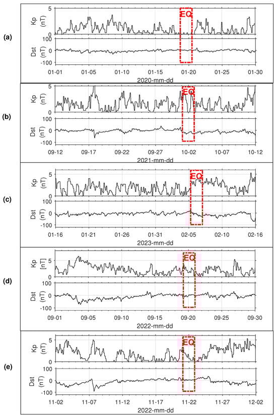
Figure 2. Shows the Dst index and Kp index corresponding to several examples given in the text. Specifically, (a–c) correspond to Figure 3, Figure 4 and Figure 5, while (d,e) correspond to the EQ cases in Section 3.4.

3. Results

3.1. Electron Spatial Distribution Evolution Related to EQs

The revisiting period of the CSES is 5 days, that is, every 5 days the satellite can complete global Earth coverage. Therefore, we used a set of 5 days of data to map the smoothed flux of the energetic particles near the epicenter. In addition, we divided the energy range into 0.1–0.3 Mev and 0.3–3.0 MeV and split the pixels in

1^{\circ} \times 1^{\circ}

. We also separated the night–side and day-side data in the statistics. To simplify the data processing, each month was divided into six sets: from the 1st to the 5th, the 6th to the 10th, and so on until the 26th to the 30th. The set in which the EQ date falls was regarded as at the time of the EQ (refer to Figure 3d, Figure 4d and Figure 5d). The forward sets were 5 days before the EQ (refer to Figure 3c, Figure 4c and Figure 5c), 10 days before the EQ (refer to Figure 3b, Figure 4b and Figure 5b) and 15 days before the EQ (refer to Figure 3a, Figure 4a and Figure 5a); the last set was 5 days after the EQ (refer to Figure 3e, Figure 4e and Figure 5e). The criterion for anomaly identification is from the second part in the article. We have marked the anomalies with red arrows in the figures.

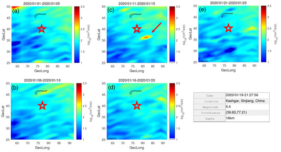
Figure 3. (a–e) are the night–side electron flux maps of 0.1–0.3 MeV for different period of the M 6.4 earthquake in Kashgar, Xinjiang, 19 January 2020. The red star indicates the epicenter and the arrow is the place of the flux anomaly.

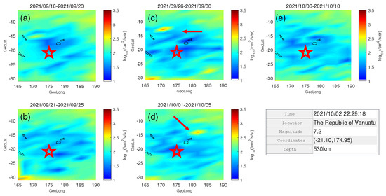
Figure 4. (a–e) are the night–side electron flux maps of 0.1–0.3 MeV for different period of the Vanuatu Islands M 7.2 earthquake on 2 October 2021. The red star indicates the epicenter and the arrow is the place of the flux anomaly.

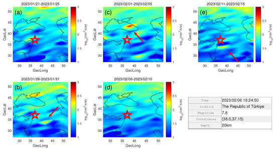
Figure 5. (a–e) are the night–side electron flux maps of 0.1–0.3 MeV for different period of the M 7.4 earthquake in Turkey on 6 February 2023. The red star indicates the epicenter and the arrow is the place of the flux anomaly.

Figure 3 illustrates the global distribution of high–energy electrons in the 0.1–0.3 MeV range on the night side during the M 6.4 EQ in Kashgar, Xinjiang, on 19 January 2020. Notably, there was a significant increase in the electron flux, approximately 500 km southeast of the epicenter, starting approximately 5 days before the EQ. This increase was almost 1 order of magnitude higher than in the other regions. Figure 4 displays the spatial distribution of the 0.1–0.3 MeV electron flux for the M 7.2 EQ in the Vanuatu Islands on 2 October 2021. Five days prior to the EQ, a slight increase in the 0.1–0.3 MeV electron flux on the night side was observed around 600 km northwest of the epicenter. Five days after the EQ, an anomaly occurred approximately 800 km northeast of the epicenter, resulting in an electron flux increase of approximately 0.5 orders of magnitude. Figure 5 presents the evolution of the electron flux during the EQ in Turkey on 6 February 2023. Around 10 days before the EQ, an anomalous electron flux increase of approximately 0.5 orders of magnitude was observed roughly 500 km southeast of the epicenter. Five days before the EQ, another anomaly appeared about 800 km northeast of the epicenter, while five days after the EQ, an anomaly manifested approximately 300 km south of the epicenter. In addition, to ensure that these anomalies are not attributed to space weather perturbations, we have attached the Dst index and Kp index at the time of these three EQs, in Figure 2a–c.

3.2. Time Evolution of Electrons Flux Related with EQs

In addition to the spatial evolution, we also studied the temporal evolution of the energetic particles at the time of the EQ. We calculated the average and maximum fluxes of the energetic particles in the orbits that pass within 10

^{\circ}

of the longitude and latitude near the epicenter each day. The blank data are due to the absence of observations, which is related to the orbit of the satellite. Figure 6 shows the daily variation in the 0.1–0.3 MeV electron flux during the M 7.0 EQ in the Solomon Islands on 22 November 2022. It can be seen that on 21 November, the day before the EQ, the maximum electron flux level exhibited a significant enhancement of approximately 0.5 orders of magnitude compared to the background value. In comparison with the Dst index, this enhancement was not from space weather perturbations.

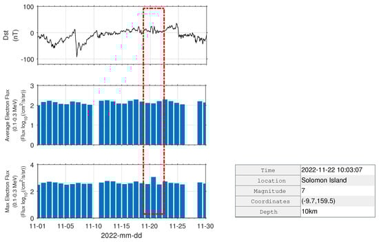
Figure 6. 0.1–0.3 MeV daily variation in electron flux in the Solomon Islands M 7.0 earthquake on 22 November 2022. Max electron flux means the maximum flux of energetic particles in orbits that pass within 10° of the longitude and latitude near the epicenter every day. The red box highlight the electron flux anomaly.

3.3. Statistical Results of High–Energy Particle Disturbance Characteristics before Strong EQs

Using the two statistical methods outlined above, we conducted a spatial and temporal analysis of 78 cases. We excluded 16 cases from this analysis due to the effects of the space weather and the high-latitude outer radiation belts. The remaining 62 cases are included in Table 2, where we present their analyses, including the magnitude, latitude, longitude, and anomalies. In 39 out of 62 cases, anomalies were detected. Approximately 62.9% was the probability of observing an anomaly in an energetic particle flux that is related to an EQ.

To investigate the attributes of the spatially energetic particles precipitation due to EQs, we conducted a separate count of the perturbations in both time and space. Concerning unusual perturbations manifested over time, we integrated the spatial distribution development depicted in Figure 3, Figure 4 and Figure 5 and the daily variation in the particle fluxes in Figure 7. For example, Figure 3 shows the spatial distribution of similarly anomalous particles from 11 January 2020 to 15 January 2020 following the 19 January 2020 EQ in Gashi County, Kashgar, Xinjiang. We believe that the electron flux anomalies in this EQ were detected 4–8 days before the EQ. Out of the 78 EQ cases, we encountered 114 time anomalies. Figure 7 displays that the highest number of anomalies appeared on the day of the EQ, 16 times more than average. Moreover, several anomalies were noted within the 5–day period preceding the EQ.

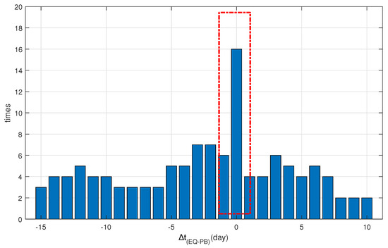
Figure 7. This figure shows the time difference between the time of electron precipitation and the earthquake. There is a clear peak occurring on the day of the earthquake (highlighted in red box), and it is most likely to have an increased particle flux on the day of the earthquake.

We also counted the spatial distribution, and the results are shown in Figure 8. This figure is a statistical orientation map from 23 anomalies, which come from 20 cases. In addition, several anomalies may occur in one case. For example, in Figure 4c,d, the particle fluxes show anomalies at different locations at both 5 days before and 5 days from the current time of the EQ, and we will count this case twice. In terms of orientation, the most anomalies appear in the northeast direction as well as in the east. By counting, there are 7 times in the northeast and 6 times in the east, and they are 56% of the total number. In terms of distance, most of the anomalies appear in the 600–900 km range, with 11 times, which is a percentage of

47 %

.

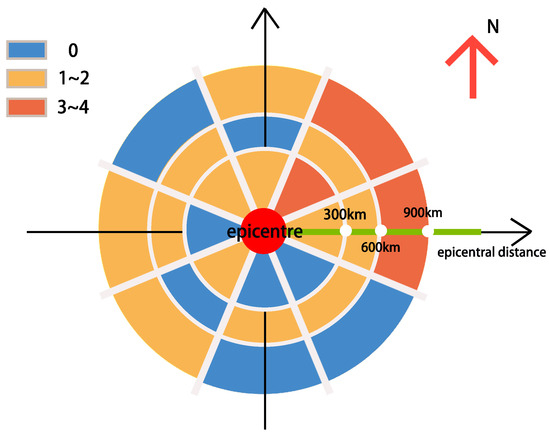
Figure 8. This figure shows the spatial distribution of the electron flux anomalies, statistically in both orientation and distance. It can be seen that from the orientation, northeast and east are the directions where the majority of anomalies arise. In terms of distance, the perturbations are most frequently found at a distance of 600 km–900 km from the epicenter, with 11 times, which is a percentage of

47 %

.

This phenomenon is consistent with the distribution of the electron precipitation belt caused by the NWC, a naval transmission ground-based station in northwest Australia. The artificial ground-based signal propagates upward from the ground, reaches the ionosphere, and has wave–particle interactions with high–energy particles. It will cause high–energy electron precipitation in the energy range of 0.1–0.3 MeV of the particles, mainly through pitch–angle scattering. The three adiabatic motions of high–energy electrons are cyclotron motion, bouncing motion, and drifting motion. The ground electromagnetic signal mainly propagates upward and interacts with the high–energy electrons performing a bouncing motion along the magnetic line, and the electrons will be precipitated downward into the atmosphere. In addition, the electrons move from west to east in the drifting direction. This principle can explain how the sunken energetic electrons are mainly distributed in the northeast direction of the wave source as in Figure 9, which is similar to the NWC electron precipitation belt.

Figure 9. Figure shows the NWC electron precipitation belts between L-shells of L = 1.4 and L = 1.8 labeled by the blue dotted line on the top panel. The following panels show the wisp electron precipitation structure and energy spectrum. The red box indicates NWC electron precipitation belts.

3.4. Possible Mechanism: Wave–Particle Interactions in Earthquakes

In the wave–particle coupling theory, when the electromagnetic wave frequency and high–energy particle cyclotron frequency in the radiation belt satisfies some conditions, the electromagnetic wave can interact with the high–energy particles following resonance. This effect causes the pitch–angle scattering of high–energy particles and the formation of particle precipitation. Therefore, the anomalous precipitation of the high–energy particle flux during the EQ may be accompanied with electromagnetic wave perturbations and wave–particle interactions.

On 20 September 2022, at 02:05, a M 7.5 EQ occurred in Mexico, at (

18 . 30^{\circ}, - 103 . 20^{\circ}

) in the geographical coordinate system, with a depth of 10 km. Figure 10 shows the observations of the CSES passing over the epicenter on the same day of the EQ with orbit number 257130. Figure 10a shows the observations of the ELF waves from the SCM payload, which observed anomalous electromagnetic wave perturbations above the epicenter and at its magnetic conjugate point. Figure 10b shows the HEPP–L observations of electrons with energies of 0.1–0.3 MeV, 0.3–1.0 MeV, and 1.0–3.0 MeV. Near the epicenter, we can observe an abnormal enhancement of the 0.1–0.3 MeV high–energy electrons flux of about 0.5 orders of magnitude. Figure 10c shows the high–energy particle energy spectrum, and we can notice that the high–energy particles were precipitated in the low energy band, about 0.1 MeV or below.

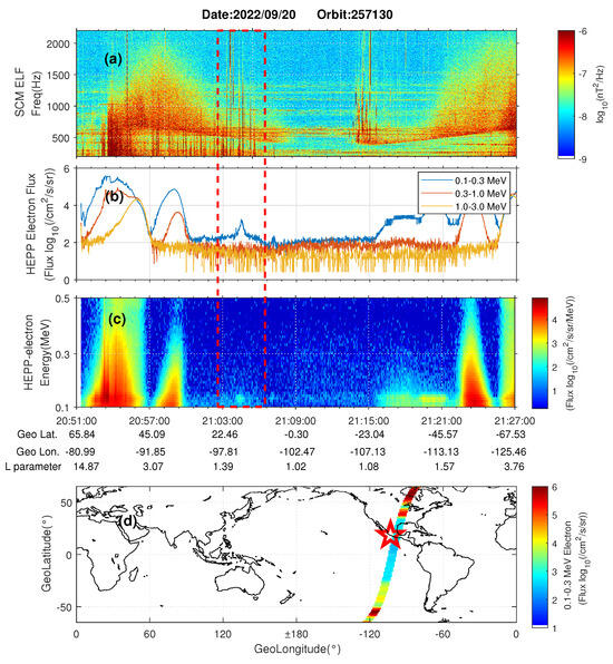
Figure 10. This figure shows the electromagnetic ELF wave perturbations and energetic particle precipitation from CSES detection during the M 7.5 earthquake in Mexico on 20 September 2022. On (a) is shown the ELF wave data from SCM payload. (b) is from the data HEPP–L, and the three lines indicate the energetic particle fluxes of 0.1–0.3 MeV, 0.3–1.0 MeV, and 1.0–3.0 MeV. On (c) is shown the electron energy spectrum of one orbit. On (d) is shown the orbit track of 257130, which is a descending orbit. The red box in (a–c) indicates a simultaneous anomaly for both ELF–wave and electron flux. The red star in (d) indicates the epicenter.

Furthermore, we have found another similar sample indicating wave–particle interactions during a M 7.0 EQ, which occurred on 22 November 2022, in the Solomon Islands, at location (

- 9 . 7^{\circ}, 159 . 5^{\circ}

) with a depth of 10 km. Two days before the EQ, the unusual electromagnetic waves and energetic particle perturbations were observed at orbit 266290. Figure 11a shows the observations of ULF waves from the SCM payload, similar to the previous example, and it also shows an anomaly at the epicenter and magnetic conjugate point. Figure 11b,c demonstrate that HEPP–L has observed significant energetic particle precipitation above the epicenter, but it is not very significant at the magnetic conjugate point.

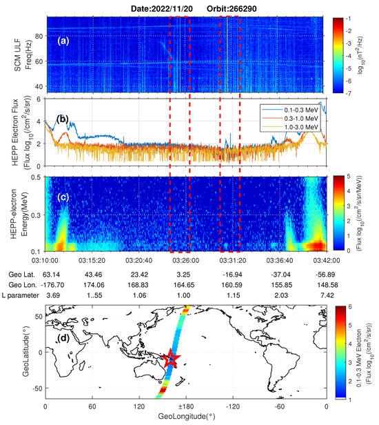
Figure 11. This figure shows another case of EQ wave–particle interaction, the Solomon Islands M 7.0 EQ on 22 November 2022. On (a) is shown the ULF wave data from SCM payload. (b) is from the data HEPP–L, and the three lines indicate the energetic particle fluxes of 0.1–0.3 MeV, 0.3–1.0 MeV, and 1.0–3.0 MeV. On (c) is shown the electron energy spectrum of one orbit. On (d) is shown the orbit track of 257130, which is a descending orbit. The red box in (a–c) indicates a simultaneous anomaly for both ULF–wave and electron flux. The red star in (d) indicates the epicenter.

4. Conclusions and Discussion

It is known that abnormal electromagnetic waves can be observed on the ground and in space before strong EQs. However, the origin of the electromagnetic waves and the principle of a lithosphere–ionosphere interaction have not been clearly explained due to the lack of enough statistical events. The CSES is the first satellite which specializes in monitoring electromagnetic disturbances in the ionosphere for the purpose of electromagnetic prediction of EQs in China. Based on the CSES data, we calculated 78 strong EQs from September 2018 to February 2023, including M 7.0 and over globally and M 6.0 and over in the major EQ regions in China. We analyzed the energetic particle flux data within ±10

^{\circ}

longitude and latitude above the epicenter and counted the energetic particle flux data from 15 days before to about 5 days after the quake and analyzed the time and space information of the anomalies distribution. Here, we conclude the main points as follows:

Among the 78 EQ cases, we excluded 16 cases from the statistical work. In the remaining 62 cases, 39 cases showed electron flux anomalies, which included spatial distribution or temporal distribution, and possibly both. Overall, the probability of EQ–related electron flux anomalies was 62%.
From the time distribution, the highest probability of anomalies was found on the current day of the EQ, with a total of 16 in 78 EQ cases. In addition, there were many anomalies that occurred during the 5 days before the EQ.
We also investigated the spatial distribution of the perturbation. The northeast was the most likely direction to show anomalies, followed by the east. This phenomenon was consistent with the distribution of electron precipitation belt caused by the ground stations NWC, which is a wisp.
In terms of distance, the largest probability of anomalous electron precipitation occurred within the range of about 600–900 km from the epicenter, with 11 times, which is a percentage of $47 %$ .
The anomalous precipitation of the high–energy particle flux during the EQ may be accompanied with electromagnetic wave perturbations and wave–particle interactions. We also presented two earthquake cases accompanied by anomalous electromagnetic waves. Electromagnetic waves excited by earthquakes interact with electrons in the radiation belt in a wave–particle interaction, which may be a probable explanation for the generation of electron precipitation during EQs. More research will be carried out for this part in the future.

Therefore, based on 5 years of CSES data, we performed the statistical research of the electron flux anomalies associated with EQs and obtained many valuable conclusions. However, the data sample of the earthquake events is far from enough. The second satellite CSES–02 will be launched in 2024. We will continue to accumulate more earthquake events and improve the analysis method to optimize the earthquake–ionosphere disturbance research. We can also make a conjecture if we can try to predict EQs from the flux of the energetic particles in the radiation belts. Of course, while we are confident in these results, visual interpretation is not objective enough and inefficient in practical applications. In the next work, we will also develop image recognition algorithms to identify anomalies using artificial intelligence. Simultaneously, we will continue to develop the wave–particle interaction theoretical model to explore the mechanism explanation and application in earthquake monitoring and prediction in the future.

Author Contributions

L.W. performed the data process and wrote the original manuscript version. Z.Z. (Zhenxia Zhang) put forward the main idea and led the whole analysis process and manuscript writing of this work. Z.Z. (Zeren Zhima), X.S., W.C., R.Y., F.G., N.Z., H.C., and D.W. provided consultation on the idea and manuscript writing of the work. All authors have read and agreed to the published version of the manuscript.

Funding

This study was supported by grants from the National Natural Science Foundation of China (NNSFC) (41904149 and 12173038), the Asia-Pacific Space Cooperation Organization Project (APSCO-SP/PM-EARTHQUAKE), research grants from the National Institute of Natural Hazards, Ministry of Emergency Management of China (Grant Number: 2021-JBKY-11), and the Stable-Support Scientific Project of China Research Institute of Radiowave Propagation (A132001W07).

Data Availability Statement

The ZH-1 satellite data can be downloaded from the Internet at https://www.leos.ac.cn of the Data Service term where scientists can access the data download service by registering online and filling the application form following the data policy (accessed on 18 February 2023).

Acknowledgments

We are grateful for the satellite data download.

Conflicts of Interest

The authors declare that the research was conducted in the absence of any commercial or financial relationships that could be construed as potential conflict of interest.

References

Pulinets, S.; Boyarchuk, K. Ionospheric Precursors of Earthquakes; Springer: Berlin/Heidelberg, Germany, 2004; pp. 142–149. [Google Scholar]
Aleksandrin, S.Y.; Galper, A.M.; Grishantzeva, L.A.; Koldashov, S.V.; Maslennikov, L.V.; Murashov, A.M.; Picozza, P.; Sgrigna, V.; Voronov, S.A. High–energy charged particle bursts in the near-Earth space as earthquake precursors. Ann. Geophys. 2003, 21, 597–602. [Google Scholar] [CrossRef]
Heki, K. Ionospheric electron enhancement preceding the 2011 Tohoku–Oki earthquake. Geophys. Res. Lett. 2011, 38, 456. [Google Scholar] [CrossRef]
Zhang, X.; Fidani, C.; Huang, J.; Shen, X.; Zeren, Z.; Qian, J. Burst increases of precipitating electrons recorded by the DEMETER satellite before strong earthquakes. Nat. Hazards Earth Syst. Sci. 2013, 13, 197–209. [Google Scholar] [CrossRef]
Voronov, S.A.; Galper, A.M.; Koldashov, S.V. Observation of high energy charged particle flux increases in SAA region in 10 September 1985. Cosm. Res. 1989, 27, 629–631. [Google Scholar]
Ruzhin, Y.Y.; Depueva, A.K. Seismo Precursors in Space as Plasma and Wave Anomalies. J. Atmos. Electr. 1996, 16, 271–288. [Google Scholar]
Sgrigna, V.; Carota, L.; Conti, L.; Corsi, M.; Galper, A.M.; Koldashov, S.V.; Murashov, A.M.; Picozza, P.; Scrimaglio, R.; Stagni, L. Correlations between earthquakes and anomalous particle bursts from SAMPEX/PET satellite observations. J. Atmos. Sol.-Terr. Phys. 2005, 67, 1448–1462. [Google Scholar] [CrossRef]
Parrot, M.; Berthelier, J.J.; Lebreton, J.P.; Sauvaud, J.A.; Santolík, O.; Blecki, J. Examples of unusual ionospheric observations made by the DEMETER satellite over seismic regions. Phys. Chem. Earth 2006, 31, 486–495. [Google Scholar] [CrossRef]
Zhang, Z.X.; Wang, C.Y.; Shen, X.H.; Li, X.Q.; Wu, S.G. Study of typical space wave–particle coupling events possibly related with seismic activity. Chin. Phys. B 2014, 23, 109401. [Google Scholar] [CrossRef]
Li, X.; Ma, Y.; Wang, P.; Wang, H.; Lu, H.; Zhang, X.; Huang, J.; Shi, F.; Yu, X.; Xu, Y.; et al. Study of the North West Cape electron belts observed by DEMETER satellite. J. Geophys.-Res.-Space Phys. 2012, 117, A04201. [Google Scholar] [CrossRef]
Yan, R.; Wang, L.W.; Zhang, S.Z. The electromagnetic disturbance study based on the observational data form satellite and ground station during a magnetic storm. Adv. Mater. Res. 2013, 804, 180–186. [Google Scholar] [CrossRef]
Fidani, C. Improving earthquake forecasting by correlations between strong earthquakes and NOAA electron bursts. Terr. Atmos. Ocean. Sci. 2018, 29, 1–14. [Google Scholar] [CrossRef]
Fidani, C.; Battiston, R. Analysis of NOAA particle data and correlations to seismic activity. Nat. Hazards Earth Syst. 2008, 8, 1277–1291. [Google Scholar] [CrossRef]
Roberto, B.; Vincenzo, V. First evidence for correlations between electron fluxes measured by NOAA-POES satellites and large seismic events. Nucl. Phys. B-Proc. Suppl. 2013, 249–257, 243–244. [Google Scholar]
Pulinets, S.A.; Boyarchuk, K.A.; Hegai, V.V.; Kim, V.P.; Lomonsov, A.M. Quasielectrostatic model of atmosphere–thermosphere– ionosphere coupling. Adv. Space Res. 2000, 26, 1209–1218. [Google Scholar] [CrossRef]
Sorokin, V.M.; Chmyrev, V.M.; Yaschenko, A.K. Electrodynamic model of the lower atmosphere and the ionosphere coupling. Atmos. Sol.-Terr. Phys. 2001, 63, 1681–1691. [Google Scholar] [CrossRef]
Sorokin, V.M.; Yaschenko, A.K.; Hayakawa, M.A. Perturbation of DC electric fifield caused by light ion adhesion to aerosols during the growth in seismic-related atmospheric radioactivity. Nat. Hazards Earth Syst. 2007, 7, 155–163. [Google Scholar] [CrossRef]
Zhao, S.; Zhang, X.M.; Zhao, Z.; Shen, X. The numerical simulation on ionospheric perturbations in electric field before large earthquakes. Ann. Geophys. 2014, 32, 1487–1493. [Google Scholar] [CrossRef][Green Version]
Anagnostopoulos, G.C.; Vassiliadis, E.; Pulinets, S. Characteristics of flux-time profiles, temporal evolution, and spatial distribution of radiation-belt electron precipitation bursts in the upper ionosphere before great and giant earthquakes. Ann. Geophys. 2012, 55, 1. [Google Scholar] [CrossRef]
Chakraborty, S.; Sasmal, S.; Basak, T.; Chakrabarti, S.K. Comparative study of charged particle precipitation from Van Allen radiation belts as observed by NOAA satellites during a land earthquake and an ocean Earthquake. Adv. Space Res. 2019, 64, 719–732. [Google Scholar] [CrossRef]
Summers, D.; Ma, C.A. A model for generating relativistic electrons in the Earth’s inner magnetosphere based on gyroresonant wave-particle interactions. J. Geophys. Res. 2020, 105, 2625–2639. [Google Scholar] [CrossRef]
Frolov, V.L.; Akchurin, A.D.; Bolotin, I.A.; Ryabov, A.O.; Berthelier, J.J.; Parrot, M. Precipitation of Energetic Electrons from the Earth Radiation Belt Stimulated by High-Power HF Radio Waves for Modification of the Midlatitude Ionosphere. Radiophys. Quantum Electron. 2020, 62, 571–590. [Google Scholar] [CrossRef]
Zhang, Z.X.; Li, X.Q.; Chen, L.J. North west cape-induced electron precipitation and theoretical simulation. Chin. Phys. B 2016, 25, 119401. [Google Scholar] [CrossRef][Green Version]
Parrot, M. Statistical study of ELF/VLF emissions recorded by a low-altitude satellite during seismic events. J. Geophys. Res. 1994, 99, 23339–23347. [Google Scholar] [CrossRef]
Parrot, M. VLF emissions associated with earthquakes and observed in the ionosphere and the magnetosphere. Earth Planet. Inter. 1989, 57, 86–99. [Google Scholar] [CrossRef]
Wang, Q.; Huang, J.; Zhao, S.; Zhima, Z.; Yan, R.; Lin, J.; Yang, Y.; Chu, W.; Zhang, Z.; Lu, H.; et al. The electromagnetic anomalies recorded by CSES during Yangbi and Madoi earthquakes occurred in late May 2021 in west China. Nat. Hazards Res. 2022, 1, 10. [Google Scholar] [CrossRef]
Yan, R.; Zhima, Z.; Xiong, C.; Shen, X.; Huang, J.; Guan, Y.; Zhu, X.; Liu, C. Comparison of Electron Density and Temperature from the CSES Satellite With Other Space-Borne and Ground-Based Observations. J. Geophys. Res. Space Phys. 2020, 125, e2019JA027747. [Google Scholar] [CrossRef]
Yan, R.; Xiong, C.; Zhima, Z.; Shen, X.; Liu, D.; Liu, C.; Guan, Y.; Zhu, K.; Zheng, L.; Lv, F. Correlation Between Ne and Te Around 14:00 LT in the Topside Ionosphere Observed by CSES, Swarm and CHAMP Satellites. Front. Earth Sci. 2022, 10, 860234. [Google Scholar] [CrossRef]
Zhima, Z.; Hu, Y.; Shen, X.; Chu, W.; Piersanti, M.; Parmentier, A.; Zhang, Z.; Wang, Q.; Huang, J.; Zhao, S.; et al. Storm-Time Features of the Ionospheric ELF/VLF Waves and Energetic Electron Fluxes Revealed by the China Seismo-Electromagnetic Satellite. Appl. Sci. 2021, 11, 2617. [Google Scholar] [CrossRef]
Zhima, Z.; Hu, Y.; Pierstanti, M.; Shen, X.; De Santis, A.; Yan, R.; Yang, Y.; Zhao, S.; Zhang, Z.; Wang, Q. The seismic electromagnetic emissions during the 2010 Mw 7.8 Northern Sumatra Earthquake revealed by DEMETER satellite. Front. Earth Sci. 2020, 8, 459. [Google Scholar] [CrossRef]
Zhima, Z.; Yan, R.; Lin, J.; Wang, Q.; Yang, Y.; Lv, F.; Huang, J.; Cui, J.; Liu, Q.; Zhao, S.; et al. The Possible Seismo-Ionospheric Perturbations Recorded by the China-Seismo-Electromagnetic Satellite. Remote Sens. 2022, 14, 905. [Google Scholar] [CrossRef]
Zhu, K.; Zheng, L.; Yan, R.; Shen, X.; Zeren, Z.; Xu, S.; Chu, W.; Liu, D.; Zhou, N.; Guo, F. Statistical study on the variations of electron density and temperature related to seismic activities observed by CSES. Nat. Hazards Res. 2021, 1, 88–94. [Google Scholar] [CrossRef]
Shen, X.H.; Zhang, X.M.; Yuan, S.G.; Wang, L.W.; Cao, J.B.; Huang, J.P. The state-of-the-art of the China Seismo-Electromagnetic Satellite mission. Sci. China Technol. Sci. 2018, 61, 634–642. [Google Scholar] [CrossRef]
Li, X.Q.; Xu, Y.B.; An, Z.H.; Liang, X.H.; Wang, P.; Zhao, X.Y.; Wang, H.Y.; Lu, H.; Ma, Y.Q.; Shen, X.H.; et al. The high–energy particle package onboard CSES. Radiat. Detect. Technol. Methods 2019, 3, 22. [Google Scholar] [CrossRef]
Zhang, Z.; Li, X.; Wang, L.; Zhima, Z.; Shen, X.; Yuan, S.; An, Z.; Xu, Y.; Liang, X.; Zhang, D.; et al. Evaluation of the proton contamination to MeV electrons by solar proton events based on CSES observations. Ournal Geophys. Res. Space Phys. 2022, 127, e2022JA030550. [Google Scholar] [CrossRef]
Cao, J.; Zeng, L.; Zhan, F.; Wang, Z.; Wang, Y.; Chen, Y.; Meng, Q.; Ji, Z.; Wang, P.; Liu, Z. The electromagnetic wave experiment for CSES mission: Search coil magnetometer. Sci. China Technol. 2018, 61, 653–658. [Google Scholar] [CrossRef]
Dobrovosky, I.R.; Zubkov, S.I.; Myachkin, V.I. Estimation of the size of earthquake preparation zones. Pageoph 1979, 117, 1025–1044. [Google Scholar] [CrossRef]

Figure 1. Global Distribution of 78 Earthquakes Observed by CSES from September 2018 to February 2023.

Figure 2. Shows the Dst index and Kp index corresponding to several examples given in the text. Specifically, (a–c) correspond to Figure 3, Figure 4 and Figure 5, while (d,e) correspond to the EQ cases in Section 3.4.

Figure 3. (a–e) are the night–side electron flux maps of 0.1–0.3 MeV for different period of the M 6.4 earthquake in Kashgar, Xinjiang, 19 January 2020. The red star indicates the epicenter and the arrow is the place of the flux anomaly.

Figure 4. (a–e) are the night–side electron flux maps of 0.1–0.3 MeV for different period of the Vanuatu Islands M 7.2 earthquake on 2 October 2021. The red star indicates the epicenter and the arrow is the place of the flux anomaly.

Figure 5. (a–e) are the night–side electron flux maps of 0.1–0.3 MeV for different period of the M 7.4 earthquake in Turkey on 6 February 2023. The red star indicates the epicenter and the arrow is the place of the flux anomaly.

Figure 6. 0.1–0.3 MeV daily variation in electron flux in the Solomon Islands M 7.0 earthquake on 22 November 2022. Max electron flux means the maximum flux of energetic particles in orbits that pass within 10° of the longitude and latitude near the epicenter every day. The red box highlight the electron flux anomaly.

Figure 7. This figure shows the time difference between the time of electron precipitation and the earthquake. There is a clear peak occurring on the day of the earthquake (highlighted in red box), and it is most likely to have an increased particle flux on the day of the earthquake.

Figure 8. This figure shows the spatial distribution of the electron flux anomalies, statistically in both orientation and distance. It can be seen that from the orientation, northeast and east are the directions where the majority of anomalies arise. In terms of distance, the perturbations are most frequently found at a distance of 600 km–900 km from the epicenter, with 11 times, which is a percentage of

47 %

.

Figure 8. This figure shows the spatial distribution of the electron flux anomalies, statistically in both orientation and distance. It can be seen that from the orientation, northeast and east are the directions where the majority of anomalies arise. In terms of distance, the perturbations are most frequently found at a distance of 600 km–900 km from the epicenter, with 11 times, which is a percentage of

47 %

.

Figure 9. Figure shows the NWC electron precipitation belts between L-shells of L = 1.4 and L = 1.8 labeled by the blue dotted line on the top panel. The following panels show the wisp electron precipitation structure and energy spectrum. The red box indicates NWC electron precipitation belts.

Figure 10. This figure shows the electromagnetic ELF wave perturbations and energetic particle precipitation from CSES detection during the M 7.5 earthquake in Mexico on 20 September 2022. On (a) is shown the ELF wave data from SCM payload. (b) is from the data HEPP–L, and the three lines indicate the energetic particle fluxes of 0.1–0.3 MeV, 0.3–1.0 MeV, and 1.0–3.0 MeV. On (c) is shown the electron energy spectrum of one orbit. On (d) is shown the orbit track of 257130, which is a descending orbit. The red box in (a–c) indicates a simultaneous anomaly for both ELF–wave and electron flux. The red star in (d) indicates the epicenter.

Figure 11. This figure shows another case of EQ wave–particle interaction, the Solomon Islands M 7.0 EQ on 22 November 2022. On (a) is shown the ULF wave data from SCM payload. (b) is from the data HEPP–L, and the three lines indicate the energetic particle fluxes of 0.1–0.3 MeV, 0.3–1.0 MeV, and 1.0–3.0 MeV. On (c) is shown the electron energy spectrum of one orbit. On (d) is shown the orbit track of 257130, which is a descending orbit. The red box in (a–c) indicates a simultaneous anomaly for both ULF–wave and electron flux. The red star in (d) indicates the epicenter.

Table 1. List of 16 EQ cases excluded.

No.	Time	M.	Lat.	Long.	Place	Space Weather	Perturbation
1	23 February 2023	7.2	37.98	73.29	Tajikistan	A moderate geomagnetic storm occurred two days before the EQ	Slightly elevated electron flux the day before the EQ
2	26 May 2022	7.2	−14.85	−70.3	Peruvian	Quiet	Near the SAA region
3	28 November 2021	7.3	−4.5	−76.7	Northern Peru	Quiet	Near the SAA region
4	23 August 2021	7	−60.55	−24.9	South Sandwich Islands	Quiet	Near the SAA region
5	14 August 2021	7	55.3	−157.75	Alaska, USA	Quiet	Near the outer radiation belt
6	13 August 2021	7.6	−57.21	−24.81	South Sandwich Islands	Quiet	Near the SAA region, near the outer radiation belt
7	29 July 2021	8.1	55.4	−158	Alaska, USA	Quiet	Near the outer radiation belt
8	24 January 2021	7	−61.7	−55.6	South Shetland Islands	Quiet	Near the SAA region
9	20 October 2020	7.5	54.74	−159.75	Alaska, USA	Quiet	Near the outer radiation belt
10	19 August 2020	7	−4.31	101.15	Sumatra, Indonesia	A moderate geomagnetic storm occurred on the day of the EQ	Slightly elevated electron flux one day after the EQ, ruled out by magnetic storms
11	22 July 2020	7.8	55.05	−158.5	Alaska, USA	Quiet	Near the outer radiation belt
12	16 June 2020	7.2	−30.8	−178.1	New Zealand Kermadec Islands	Quiet	Near the outer radiation belt
13	26 May 2019	7.8	−5.85	−75.18	Northern Peru	Quiet	Near the SAA region
14	1 March 2019	7	−14.58	−70.05	Peruvian	Quiet	Near the SAA region
15	11 December 2019	7	−58.35	−26.37	South Sandwich Islands	Quiet	Near the outer radiation belt
16	1 December 2019	7.2	61.35	−150.06	Alaska, USA	Quiet	Near the outer radiation belt

Table 2. Strong earthquakes and their related high–energy electron flux perturbations observed by CSES from September 2018 to February 2023.

No.	Time	M.	Lat.	Long.	Place	Perturbation
1	6 February 2023	7.8	37.15	36.95	Turkey	Ten days before the EQ, an anomaly occurred 500 km southeast of the epicenter. Five days before the EQ, an anomaly occurred 800 km northeast of the epicenter. Five days after the EQ, an anomaly appeared 300 km south of the epicenter.
2	30 January 2023	6.1	40.01	82.29	Aksu, Xinjiang	No apparent abnormality.
3	18 January 2023	7	2.8	127.1	Indonesia	Two days before the EQ, there was an anomaly in the daily maximum electron flux in the range of 0.3–3.0 MeV, night side.
4	10 January 2023	7.6	−7.2	130.1	Indonesia	No apparent abnormality.
5	8 January 2023	7	−14.95	166.8	Vanuatu	Fifteen days before the EQ, there was an anomaly in the daily maximum electron flux in the range of 0.1–0.3 MeV, night side.
6	22 November 2022	7	−9.7	159.5	Solomon Island	Fifteen days before the EQ, there was a slight rise in the night–side 0.1–0.3 MeV electron flux about 1000 km east of the epicenter.
7	11 November 2022	7.4	−19.25	−172.05	Tonga Islands	Ten days before the EQ, an anomaly occurred 500 km in east of the epicenter.
8	20 September 2022	7.5	18.3	−103.2	Mexico	Twelve days before the EQ, there was an anomaly in the daily maximum electron flux in the range of 0.3–3.0 MeV, day side.
9	18 September 2022	6.9	23.15	121.3	Hualien, Taiwan	On the day of the EQ, there was an anomaly in the daily maximum electron flux in the range of 0.3–3.0 MeV, day side.
10	11 September 2022	7.6	−6.3	146.55	Papua New Guinea	Five days after the EQ, an anomaly occurred directly above the epicenter.
11	5 September 2022	6.8	29.59	102.08	Luding, Sichuan	On the day of the EQ, there was an anomaly in the daily maximum electron flux in the range of 0.3–3.0 MeV, day side.
12	27 July 2022	7	17.7	120.55	Philippine	No apparent abnormality.
13	10 June 2022	6	32.25	101.82	Malcolm, Sichuan	On the day of the EQ, there was an anomaly in the daily maximum electron flux in the range of 0.3–3.0 MeV, day side.
14	1 June 2022	6.1	30.37	102.94	Ya’an, Sichuan	No apparent abnormality.
15	9 May 2022	6.2	24.01	122.51	Hualien, Taiwan	No apparent abnormality.
16	26 March 2022	6	38.5	97.33	Haixi, Qinghai	On the day of the EQ, there was an anomaly in the daily maximum electron flux in the range of 0.3–3.0 MeV, night side.
17	23 March 2022	6.6	23.45	121.55	Taitung, Taiwan	No apparent abnormality.
18	16 March 2022	7.4	37.65	141.95	Japan	No apparent abnormality.
19	8 January 2022	6.9	37.77	101.26	Haibei, Qinghai	No apparent abnormality.
20	3 January 2022	6.4	24	122.39	Hualien, Taiwan	On the day of the EQ, there was an anomaly in the daily maximum and average electron flux in the range of 0.3–3.0 MeV, night side.
21	30 December 2021	7.5	−7.75	127.6	Banda Sea	On the day of the EQ, there was an anomaly in the daily maximum and average electron flux in the range of 0.3–3.0 MeV, night side. Five days after the EQ, an anomaly occurred directly above the epicenter and 500 km west of the epicenter.
22	14 December 2021	7.3	−7.6	122.2	Flores Sea	In the 2–3 days of the EQ, there was an anomaly in the daily maximum electron flux in the range of 0.3–3.0 MeV, day side.
23	24 October 2021	6.3	24.55	121.8	Yilan, Taiwan	Five days after the EQ, an anomaly occurred 300 km northeast of the epicenter.
24	2 October 2021	7.2	−21.1	174.95	Vanuatu	In the 5 days of the EQ, an anomaly occurred 600 km northeast of the epicenter. Five days after the EQ, an anomaly occurred 800 km northeast of the epicenter.
25	16 September 2021	6	29.2	105.34	Luzhou, Sichuan	No apparent abnormality.
26	8 September 2021	7.1	17.12	−99.6	Mexico	Five days before the EQ, an anomaly occurred 800 km east of the epicenter.
27	18 August 2021	7	−14.79	167.04	Vanuatu	Five days after the EQ, an anomaly occurred 300 km east of the epicenter. For 2–3 days of the EQ, there was an anomaly in the daily maximum electron flux in the range of 0.3–3.0 MeV, night side.
28	14 August 2021	7.3	18.35	−73.45	Haiti	On the day of the EQ, there was an anomaly in the daily maximum electron flux in the range of 0.3–3.0 MeV, night side.
29	22 May 2021	7.4	34.59	98.34	Mado, Qinghai	On the day of the EQ, there was an anomaly in the daily maximum electron flux in the range of 0.3–3.0 MeV, day side.
30	21 May 2021	6.4	25.67	99.87	Dali, Yunnan	On the day of the EQ, there was an anomaly in the daily maximum electron flux in the range of 0.3–3.0 MeV, night side.
31	18 April 2021	6.1	23.94	121.43	Hualien, Taiwan	On the day of the EQ, there was an anomaly in the daily maximum electron flux in the range of 0.3–3.0 MeV, dayside.
32	20 March 2021	7	38.43	141.84	Japan	On the day of the EQ, there was an anomaly in the daily maximum electron flux in the range of 0.3–3.0 MeV, night side.
33	19 March 2021	6.1	31.94	92.74	Nagchu, Tibet	The 5 days of the EQ, an anomaly occurred 500 km northeast of the epicenter.
34	5 March 2021	7.8	−29.51	−177.04	New Zealand Kermadec Islands	Ten days before the EQ, an anomaly occurred 300 km southeast of the epicenter.
35	13 February 2021	7.1	37.7	141.8	Japan	Ten days before the EQ, an anomaly occurred 100 km north of the epicenter.
36	10 February 2021	7.4	−23.05	171.5	Loyalty Islands	Ten days before the EQ, an anomaly occurred 300 km northeast of the epicenter.
37	17 July 2020	7	−7.86	147.7	Papua New Guinea	Fifteen days before the EQ, an anomaly occurred 300 km south of the epicenter. One day and three days before the EQ, there was an anomaly in the daily maximum electron flux in the range of 0.3–3.0 MeV, night side.
38	26 June 2020	6.4	35.73	82.33	Hotan, Xinjiang	The 5 days of the EQ, an anomaly occurred 1000 km northeast of the epicenter.
39	23 June 2020	7.4	16.14	−95.75	Mexico	No apparent abnormality.
40	18 June 2020	7.3	−33.35	−177.85	New Zealand Kermadec Islands	No apparent abnormality.
41	6 May 2020	7.2	−6.93	130.07	Indonesia	On the day of the EQ, there was an anomaly in the daily maximum electron flux in the range of 0.3–3.0 MeV, day side.
42	25 March 2020	7.5	48.93	157.74	Kuril island chain	No apparent abnormality.
43	13 February 2020	7	45.6	148.95	Kuril island chain	No apparent abnormality.
44	29 January 2020	7.7	19.46	−78.79	Southern Cuban waters	No apparent abnormality.
45	19 January 2020	6.4	39.83	77.21	Qeshqer, Xinjiang	Two days before the EQ, there was an anomaly in the daily maximum electron flux in the range of 0.3–3.0 MeV, day side. Five days before the EQ, an anomaly occurred 500 km southeast of the epicenter.
46	15 November 2019	7.2	1.55	126.48	Indonesia	On the day of the EQ, there was an anomaly in the daily maximum electron flux in the range of 0.3–3.0 MeV, day side.
47	8 August 2019	6.4	24.52	121.96	Yilan, Taiwan	Five days before the EQ, an anomaly occurred 400 km southnortheast of the epicenter.
48	14 July 2019	7.1	−0.52	128.17	Indonesia	No apparent abnormality.
49	24 June 2019	7.3	−6.36	129.24	Haiti	No apparent abnormality.
50	17 June 2019	6	28.34	104.9	Yibin, Sichuan	No apparent abnormality.
51	14 May 2019	7.6	−4.15	152.52	New Britain region	Three days before the EQ, there was an anomaly in the daily maximum electron flux in the range of 0.3–3.0 MeV, day side. Ten days before the EQ, an anomaly occurred 500 km west of the epicenter.
52	7 May 20197	7.1	−6.96	146.49	Papua New Guinea	No apparent abnormality.
53	24 April 2019	6.3	28.4	94.61	Linzhi, Tibet	On the day of the EQ, there was an anomaly in the daily maximum electron flux in the range of 0.3–3.0 MeV, night side.
54	18 April 2019	6.7	24.02	121.65	Hualien, Taiwan	Three days after the EQ, there was an anomaly in the daily maximum electron flux in the range of 0.3–3.0 MeV, night side.
55	22 February 2019	7.5	−2.15	−76.91	Ecuador	No apparent abnormality.
56	26 November 2018	6.2	23.28	118.6	Taiwan Strait	The 5 days of the EQ, an anomaly occurred 1000 km east of the epicenter.
57	26 October 2018	7	37.51	20.51	Ionian Sea	No apparent abnormality.
58	23 October 2018	6	24.01	122.65	Hualien, Taiwan	The 5 days of the EQ, an anomaly occurred 800 km east of the epicenter.
59	11 October 2018	7.1	−5.7	151.25	Papua New Guinea	Ten days before the EQ, an anomaly occurred 10,300 km southwest of the epicenter.
60	28 September 2018	7.4	−0.25	119.9	Indonesia	No apparent abnormality.
61	10 September 2018	7	−31.95	−179.25	Kermadec Islands	No apparent abnormality.
62	6 September 2018	7.8	−18.45	179.35	Fiji	No apparent abnormality.

Disclaimer/Publisher’s Note: The statements, opinions and data contained in all publications are solely those of the individual author(s) and contributor(s) and not of MDPI and/or the editor(s). MDPI and/or the editor(s) disclaim responsibility for any injury to people or property resulting from any ideas, methods, instructions or products referred to in the content.

© 2023 by the authors. Licensee MDPI, Basel, Switzerland. This article is an open access article distributed under the terms and conditions of the Creative Commons Attribution (CC BY) license (https://creativecommons.org/licenses/by/4.0/).

Article Metrics

Citations

Article Access Statistics

Journal Statistics

Multiple requests from the same IP address are counted as one view.