1. Introduction
The current underground operation process of coal mine robots has problems such as non-transparent information about the state of the working environment, low integration and systematization, and a lack of ability to effectively respond to changes in the environmental conditions of the laneway. Underground equipment intelligence is still stuck in the robotization stage of individual pieces of equipment, and the system-wide intelligent control of the intelligent body of the underground operating machine crowd has not been formed. The reasons for the above situation are diverse. At the level of single-robot autonomy, for mobile robots of different applications such as digging, mining, transportation, inspection and rescue, key technologies such as precise robust positioning and environmental map construction under complex underground conditions have not yet been broken through to achieve autonomous navigation and autonomous operation. From the perspective of system intelligence, different work areas and types of robots cannot realize positioning and navigation and autonomous operation based on a unified coordinate system, and the efficiency of scene modeling and updating is low, which cannot meet the requirements of building a system-wide digital twin control platform, posing a great challenge to achieving the transparent and intelligent control of the underground robot crowd.
Simultaneous localization and mapping (SLAM) is a field of research that has witnessed substantial growth in the past decade, with the aim of reconstructing the scene model while simultaneously locating a robot in real-time. This technology gradually gained traction in industrial applications due to its potential to enhance autonomous systems’ capabilities. Compared to ground mobile robots, SLAM tasks for underground coal mine robots face many challenges.
Firstly, underground coal mine environments are dim and always have dust, water vapor, smoke, and other complex conditions. The visibility in mines is worse after a disaster, and the road surface is slippery and bumpy, causing the performance of conventional sensors such as lidar and cameras to degrade dramatically. There is an urgent need for high signal-to-noise ratio sensors and effective information processing to solve the problem of feature extraction and data association in a front–end manner, so that it can meet the demand for long-term robust applications under harsh underground conditions.
Secondly, confined narrow-tunnel underground spaces lead to weak texture, less structure, and large scene ambiguity. The geomagnetic and large electromagnetic interference of electromechanical equipment leads to wireless signal attenuation, shielding, NLOS, and multipath propagation, which will lead to the sensor state estimation process to introduce a large amount of false information. Reliance on a single sensor cannot meet the accuracy and reliability requirements of complex environments. The use of multi-source information fusion must address the effective use and estimation consistency of various types of noise and spurious data.
Thirdly, for robots that need geographic information guidance to perform mining operations such as digging, coal mining, drilling, transportation, etc., it is necessary to obtain the position estimation and environment model that are consistent with the geographic information. This is a prerequisite for constructing a visualized digital twin control platform based on geographic information, as well as an inevitable demand for realizing coal mining robots from single-robot autonomy to whole-system intelligence. An underground coal mine is an environment where GPS does not function and where it is difficult to obtain the global reference system, whilst the current method of determining the geodetic coordinates based on the conduction of the roadway control points by means of total station external mapping is not suitable for the application of robotic swarm operation in a large-scale scenario. New means must be used to solve the problems of the real-time matching and fusion of SLAM process and spatial location geodetic coordinates in an integrated and normalized way.
In conclusion, currently in the field of SLAM for coal mine robots, no research has been conducted to explore how to align the constructed maps with the geographic information of the underground, which is crucial for a large number of robots that need to interact with the environment to perform their operations, such as the robots used for tunneling, mining, and so on. Most of the current lidar and visual odometry can only estimate the robot’s position relative to the starting motion position, and the constructed maps do not have real geographic information and do not contain absolute position information. It needs to be manually aligned offline with coal mine electronic maps before it can be used for an underground geographic information system (GIS). Moreover, as the robot moves for a long period of time, the error will gradually accumulate, requiring frequent manual corrections to align different coordinate systems. Due to the non-institutionalized environment, complex terrain, and harsh working conditions characterizing the underground, SLAM for coal mine robots also represents a great challenge.
In this paper, we propose a new SLAM method for localization and mapping with geographic information by fusing data from LiDAR, Inertial, and UWB (LIU-SLAM) for coal mine robots. The main contributions of this paper are summarized as follows:
A new lidar relative pose factor is proposed and fused with an IMU pre-integration factor to construct a lidar-inertial odometry in a tightly coupled fashion. A new global UWB position factor and a new global range factor are designed to construct the global constraints in the global pose graph optimization in a loose-coupled fashion.
A modularized and two-layer optimization fusion framework is proposed to leverage observations from lidar, IMU, and UWB for the multi-sensor fusion SLAM, which achieves robustness, high accuracy, and aligns the estimation results with real-world online geographic information.
Extensive experiments are carried out on a practical underground garage and underground laneway by a coal mine robot to demonstrate the feasibility of proposed framework and algorithm.
2. Related Works
Underground SLAM has been studied for a long time, mainly using handheld devices [
1], mobile trolleys [
2], probe robots [
3], and mining trucks [
4] carrying sensors such as LIDAR and IMU modules for environment modeling. Tardioli et al. [
5] discussed the decade of relevant research advances in the field of underground tunneling robotics, focusing on the use of LIDAR-based, vision camera, odometry, and other SLAM methods in tunnel environments. The SubT tournament organized by the US DARPA from 2018 to 2021 is oriented to robotics applications in urban underground spaces, tunnels and natural cave environments, and related studies have proposed new solutions to typical problems in SLAM for underground scenes such as illumination changes [
6], scene degradation [
7] and alleyway feature exploitation [
8]. Ma et al. [
9] proposed a solution to solve the underground localization and map building to realize the autonomous navigation of mobile robots by using a depth camera. Chen et al. [
10] proposed a SLAM method concept for millimeter-wave radar point cloud imaging underground in coal mines, combined with deep learning to process sparse point clouds. Yang et al. [
11] investigated the roadway environment sensing method for tunneling robots based on Hector-SLAM. Li et al. [
12] proposed a lidar-based NDT-Graph SLAM method for an efficient map building task of coal mine rescue robots. Mao et al. [
13] used a measuring robot to track the coal mining machine body prism to conduct geodetic coordinates and realize coal mining machine positioning, which is an application area limited by the scanning of the measuring robot obtaining geographic information at a high cost. Overall, the research on SLAM for coal mining robots focuses on solving the initial application and performance improvement of sensors such as lidar, cameras, millimeter wave radar, etc., in specific scenarios and under specific conditions, and there is no downhole localization or map-building scheme that can be obtained in agreement with the geographic information, and the long-term localization modeling technology for the complex environment of multiple conditions coupled with the downhole still requires further exploration.
In the field of SLAM for ground mobile robots, the use of multi-sensor fusion to cope with complex environments has also become a current research feature. On the basis of pure laser odometers such as LOAM [
14] and LEGO-LOAM [
15], a large number of lidar-inertial odometry based on filtering such as LINS [
16], Faster-LIO [
17], and optimization such as LIO-mapping [
18] and LIO-SAM [
19] have been proposed, which are integrated by means of being loose coupling or tight coupling. Utilizing the rich information of images to make up for the shortcomings of a lack of laser features, a large number of laser-visual-inertial fusion methods have been further proposed, e.g., LVI-SAM [
20], R2LIVE [
21], R3LIVE [
22], LIC-Fusion [
23], LIC-Fusion2 [
24], and mVIL-Fusion [
25]. Many methods have been proposed to address degradation by combining visual and inertial information besides lidar-based information. Zhang et al. [
26] proposed the degeneracy factor of eigenvalues and eigenvectors to identify the degenerate directions in the state space. A sequential and multilayer sensor fusion pipeline was further presented in [
27] to integrate data from lidar, camera, and IMU. VIL SLAM [
28] incorporated stereo VIO to a lidar mapping system by tightly coupled fixed-lag smoothing to mitigate failures under degenerate cases of pure lidar-based approach. Both of these approaches achieved robust and accurate performance in the tunnel. However, vision-aided methods are not suitable for long-term operation under obscurity circumstances which harm vision detection and tracking. Zhen and Scherer [
29] proposed a localization approach which use an ultra-wideband (UWB) to compensate for the degeneration of lidar. They described the localizability as the virtual force and torque constraints which restrain the uncertainty of state estimation. A limitation of this work is that a map must be given a priori.
In conclusion, current underground SLAM methods only focus on localization and modeling results relative to the robot’s initial position, making it difficult to simultaneously obtain absolute geographic information in an underground coal mine, which is critical for some coal mine robotics applications.
3. System Overview
Before the methodology is introduced, we first make conventions for the definition of the coordinate system and notation and describe the system architecture.
3.1. Coordinate Systems and Notation
The establishment of underground maps that align with actual geographic information is an open problem that has been understudied in the field of SLAM to date. Most laser and visual odometers can only estimate pose relative to the starting point of the moving robot. The map built in this way will gradually deviate from the true value of the geographic information as the robot runs for a long time. The produced map does not contain absolute position information and requires manual alignment with a mine survey profile before being imported into the underground GIS. Inspired by this method, we introduce UWB observation constraints that imply absolute geographic coordinate information to realize the alignment online. The UWB anchor nodes are installed at control points or associated target points, which were accurately surveyed when the coalmine was built and contained absolute geographic information. The coordinate systems are defined in
Figure 1. The lidar frame {
L}, IMU frame {
I}, and UWB mobile node frame {
U} originate from their measurement center. World frame {
W} is the east–north–up (ENU) coordinate converted by the geographic coordinate of UWB anchor nodes in the laneway. Local frame {
O} is the gravity-aligned coordinate system which coincides with the IMU frame {
I} at the start point of the robot’s movement, the direction of which is also aligned with the
z axis direction of the world frame {
W}.
Lidar-inertial odometry provide the local pose estimation between {I} and {O}, denoted by . The extrinsic parameters between IMU with the 3D lidar and the UWB mobile node, denoted by and , are known by mechanical configuration. UWB observations provide the global position constraint in {W} denoted by . There is an invariable transformation between {O} and {W} after system initialization, denoted by , which represents the extrinsic transformation between the lidar-inertial odometry coordinate system {O} and the world coordinate system {W}. Our goal is to estimate the state of IMU in {W}, which is denoted by .
3.2. Systems Framework
In order to ensure that the system can continue to work after the failure of a single sensor and to improve the robustness of the system, two parallel sliding-window optimizers are used as the back-end to process all the sensor data. The local lidar-inertial odometry is constructed by fusing the laser and inertial data in a tightly coupled way (
Section 4), and the lidar-inertial odometry is further fused with the global UWB position and distance observation information using a loosely coupled factor graph optimization method (
Section 5), which makes the system more stable and reliable and improves the adaptability to degraded scenarios, including those with few structures and complex conditions such as bumpy roads, and enables the system to deal with the intermittent and noisy global UWB position and distance observations.
Firstly, the lidar relative position factor (
Section 4.1), the IMU pre-integration factor (
Section 4.2), and the loop closure factor (
Section 4.3) are constructed separately, and the state estimation in the local coordinate system is carried out in a tightly coupled form using a local sliding window optimizer (
Section 4.4) to achieve the construction of the lidar-inertial odometry.
Secondly, the position constraint factors (
Section 5.1) ands distance constraint factors (
Section 5.2) provided by the UWB are fused with the lidar-inertial odometry factors (
Section 5.3) in a loosely coupled manner (
Section 5.4) to achieve globally consistent map construction and precise positioning.
Meanwhile, system initialization needs to be performed when the system starts up (
Section 6). Lidar-inertial initialization and extrinsic calibration will first be performed (
Section 6.1), and then the lidar-inertial odometry in the local coordinate system can be automatically aligned with the world coordinate system (
Section 6.2).
The state estimation and map building are designed as multi-threaded parallel computation. Local submaps and global maps are constructed separately and run in different threads with different frequencies. The data from the IMU will be utilized by lidar point cloud de-distortion and pre-integration factor construction, respectively, to take advantage of its short-time and high-accuracy capabilities.
The benefit of this architecture is that, even when relying on lidar positioning is inaccurate due to scene degradation or excessively severe bumps, or when the lidar data are very noisy due to high concentrations of smoke and dust in the laneway, it is still possible to achieve usable state estimation by decreasing the weight of the lidar-inertial odometry, and utilizing the UWB position and distance observations to provide reliable positional information to enable the construction of maps. Moreover, the two optimization processes are asynchronous, with the lidar-inertial odometry executed at high frequencies used to provide high-frequency accurate position estimation, and alignment corrections in the global coordinate system periodically using the constraints provided by the UWB, which reduces the amount of computation as much as possible while ensuring global map consistency. Furthermore, this framework can be further extended with types of global observations, such as using IMUs containing magnetic sensors or observations using visual sensors, which can obtain orientation information and construct orientation constraints to participate in optimization.
The overall framework of the algorithm is shown in
Figure 2.
4. Construction of Local Optimization
The tightly coupled approach is first utilized to integrate the lidar and inertial observations. While obtaining the lidar scanning observations, the IMU observations propagate the state of motion through high frequencies for a distortion correction of the point cloud. The de-distorted point cloud is passed through area filtering and downsampled to reduce the data dimensionality. Edge and surface features are then extracted to simultaneously construct the subgraph and a local lidar relative pose factor is established, which is jointly optimized with the IMU pre-integration factor and loop closure factor in a local sliding window to perform local pose estimation with IMU zero-bias estimation.
4.1. Lidar Relative Pose Factor
4.1.1. Point Cloud Distortion Correction and Filter
The scan pattern of the mechanically rotating lidar leads to inevitable point cloud distortion when it is moving. The traditional way to address this issue is to interpolate points by corresponding timestamps between two consecutive laser sweeps under the assumption of constant motion calculated by lidar odometry. Although this approach is more efficient, this may cause problems for aggressive motion and low frequency lidar scanning, especially in a degraded scenario which easily lead to the misregistration of lidar odometry. In this paper, the high-frequency IMU measurements will be propagated to retrieve the state of lidar. Note that
i and
j are the timestamps corresponding the two consecutive lidar measurements
Si and
Sj, respectively. With the raw measurements of acceleration
and angular rate
from the IMU, the states of position
, velocity
, and orientation
in the IMU frame in a time instant
j can be propagated from the state in time instant
i by:
where the accelerations biases
and angular rates biases
are referred as constant values during each sample interval. With the offline calibrated extrinsic
between IMU and lidar, the lidar motion of current position and velocity can be predicted. The points in sweep
Sj can be rearranged by linear interpolation into a common coordinate frame at the end pose of the sweep
Sj according their corresponding timestamps. A clear advance of the prediction method is that the biases are captured from the most available result of optimization, which give a more accurate estimation for long-term operation. After point cloud correction, a region filter is used to extract points with a distance between 20 cm and 80 m. This is because further distance will produce more points parallel to the wall of the laneway and outliners which are unstable and unreliable for registration.
4.1.2. Feature Extraction
The feature extraction method of LOAM [
14] is used to extract the line features and surface features in the current point cloud by calculating the roughness of the point cloud in the local region. The point cloud obtained by lidar during a certain scanning period
k is denoted by
Pk, and the corresponding lidar coordinate system during this period is defined as
Lk, and the position coordinates of a point
in the point cloud under
Lk can be expressed as
.
S is the set of consecutive points consisting of the points in the row where point
pi is located in the point cloud
Pk. Here, |
S| is set to 10, i.e., there are five points on each side of point
pi. The following equation can be designed to evaluate the roughness of the local surface where point
pi is located:
Depending on the application environment, a feature judgment threshold can be set based on the experience gained from testing. When the roughness is greater than or less than a specific threshold, it is recognized as edge points or flat points. (i) Edge points: take the n points with the largest roughness c value and sort them as edge points with a larger curvature; (ii) Plane points: take the m points with the largest roughness c value and sort them as plane points with a smaller curvature. In order to make the point cloud features uniformly distributed in all directions, each scanning frame is divided into a number of regions, and each region extracts the n = 2 edge points with the largest roughness and the m = 4 plane points with the smallest roughness.
4.1.3. Feature Association
After obtaining a new lidar scanning frame , it is necessary to convert from the lidar coordinate system {L} to the odometry coordinate system {O}. Since the lidar is always in motion from timestamp k to k + 1, each point in the new frame corresponds to a different lidar transformation matrix. With the robot motion state predicted by the IMU, the transformed feature set can be obtained. Therefore, it is possible to look for correlations between the edge features and the surface features in the feature set in local submaps . For the edge feature i, a certain feature point is selected in . The 3D-kd tree is used to find the nearest point j in , and find the point l which is the nearest point to j but not co-located with points i and j in . Then, (j, l) is the associated feature point for edge feature i. Similarly, the nearest j to the planar feature i in and the two nearest non-collinear points m and l to j in can be found, i.e., the associated feature points (j, m, l) of the planar feature i.
For an edge point
i in frame
k + 1, the distance between this point with its correspondence edge line (
j,
l) in frame
k can be calculated by:
where
,
,
are the coordinates of edge point
i,
j, and
l in lidar frame {
L}, respectively. For a planar point
i in frame
k + 1, the distance between this point with its correspondence planar (
j,
l,
m) can be calculated by:
The following cost function is constructed to solve the optimal transformation
:
The following optimization equation can be constructed by the Levenberg–Marquardt (LM) method:
where
is the radius of the trust region,
D is the coefficient matrix, and the Jacobi matrix
. The optimal estimate is derived iteratively:
The current transformation estimate
can be obtained after convergence using the above LM optimization method. The relative transformation between
Tk and
Tk+1 is:
4.1.4. Keyframes and Submap Construction
Not every lidar frame will be added to the factor graph. Keyframes will be constructed by comparing the Euclidean norm of translation vector
and the geodesic distance of rotation matrix
with the preset thresholds to eliminate redundant information and save resources. The calculation formula of keyframe transformation can be found in the previous work [
12]. For any keyframe
Sk, the associated state is
xk, and the associated lidar features set is
. A sliding window is built to construct the submap by features with the corresponding keyframe
S0~
Si (see
Figure 3). The features in sweep
Sk,
Sk{
S0,⋯,
Sp,⋯,
Si} corresponding to timestamps 0–
i in the submap window, i.e.,
, will be transformed into the common coordinate frame corresponding to the keyframe sweep
Sp by the relative transformation
between lidar pose
and the integration pose
and then merged together into a submap
Mp. These two poses are transformed from the optimized IMU poses of
and
, by the help of the extrinsic parameters
. Finally, the submap
is built in the common coordinate frame corresponding to the pose
. The relative transformation between the following keyframe sweeps {
Sp+1, ⋯,
Si,
Sj} and
will be found to construct the lidar relative pose factors.
4.1.5. Construction of Lidar Relative Pose Factor
The lidar relative pose factor provides a constrained relationship between the new keyframe poses and the keyframe poses within the previously constructed submaps. The lidar relative pose factor involved in the optimization are the adjacent lidar keyframe poses within the optimization sliding window. The optimization objective term between adjacent poses:
where
x is the optimization variable,
xi is the motion state corresponding to keyframe
i,
xj is the motion state corresponding to keyframe
j, and
is the relative pose transformation covariance matrix.
Since the estimation process is based on the IMU coordinate system, the relative pose observations need to be converted into the IMU coordinate system:
where
is the extrinsic transformation from the IMU into the lidar coordinate system, and
is the to-be-estimated pose in the odometry coordinate system corresponding to keyframe
k. The residual between the observation and expectation of the pose transformation from keyframe
j to
i can be expressed as:
The rotational
and translational
of the relative position factor residuals are derived:
The Jacobian matrices of the relative pose factor residuals with respect to translations and rotations can be solved by deriving them in vector space and manifold space, respectively. Since the front–end alignment employs a scan-to-submap approach, the covariance of the overall scan matching is computed using the sum of the uncertainties of all successfully matched feature points. A corresponding feature point
can be obtained by projecting the feature point
of the current frame back to the submap:
and
are the relative transformations of the scan matching. The covariance calculated for all successfully matched lidar features is:
The noise matrix
can be defined as:
where
,
, and
are the noise sigma values in the
x,
y, and
z axes directions, respectively, that are simultaneously subject to noise at two points
and
, with typical values chosen to be 5 cm. The covariance matrix corresponds to the information matrix:
The information matrix for the initial motion moment is set to be 06×6. As the odometry accumulates, Equation (16) is iteratively calculated to be the information matrix that responds to the odometry uncertainty, and this matrix becomes larger as the distance traveled increases.
4.2. IMU Pre-Integration Factor
Pre-integration is developed to deal with the high-frequency IMU measurements in the graph-based visual-inertial navigation system, which was firstly proposed by Lupton et al. [
30] in Euclidean spaces. Foster et al. [
31] further derived the rotation measurements on a manifold structure and give higher accuracy and robustness results. Eckenhoff et al. [
32] presented two new closed-form inertial models and offered a better improved accuracy than the above discrete methods, especially in highly dynamic scenes. In this paper, we still discretely sample the IMU measurements because it can provide enough accuracy but computes more efficiently [
33]. The purpose of IMU pre-integration is to allow the fast processing of a large number of high-frequency inertial observations, by pre-integrating the inertial observations between selected keyframes and thus turning them into an independent relative motion constraint involved in the state estimation process.
Figure 4 shows the timestamps of the lidar and IMU observations during the pre-integration process.
A series of IMU observations between neighboring lidar keyframes establishes a kinematic constraint on the IMU pose. In this paper, a pre-integration method consistent with VINS is used, and the IMU pre-integration residual implicitly establishes a flexible constraint on the motion state between lidar keyframes
i and
j and the IMU bias estimation. Using the IMU pre-integrated observation equations, the residuals between neighboring keyframes
i and
j in the sliding window can be defined as Equation (19), with the Jacobian and covariance derivations referenced in [
33].
The cost term of the IMU pre-integration factor is:
4.3. Loop Closure Factor
Loop optimization can substantially improve the consistency of map construction. In this paper, we adopt the loop detection by odometry-based and appearance-based method which has been proposed in our previous work [
12]. The following processes are included:
- (1)
Odometry-based method: When a new keyframe is established, the factor graph is first searched and keyframes that are close in Euclidean distance to the new keyframe pose xj are found. Historical keyframes smaller than a set distance threshold will be used as candidate keyframes for loop closure, corresponding to the pose xn. Benefitting from the acquisition of geographic information in the SLAM process, the absolute position is used to assist loop closure optimization and avoid “false-positives” in ambiguous scenarios with conventional loop closure detection.
- (2)
Appearance-based method: The ICP scanning matching is used to match the point cloud of the current keyframe
with the local submap
composed of the
m frames before and after the loop candidate keyframe. Before scan matching, both the new keyframe and the local submap need to be transformed to the local lidar-inertial odometry coordinate system. The Euclidean distance root mean square minimum distance of the nearest point pair is utilized to obtain the computed fit fraction
f, which is compared with a set threshold to determine whether it is a true loop keyframe.
- (3)
Loop closure factor construction: after determining the loop keyframe, the relative transformation is calculated using Equation (8) and added to the local sliding-window optimization using the same calculation method of the lidar relative pose factor. Finally, the lidar relative pose factor, the IMU pre-integration factor, and the loop closure factor will be optimized in the local optimizer and finally be used to construct a lidar-inertial odometry factor.
4.4. Local Sliding-Window Optimization
As shown in
Figure 3, the to-be-optimized states of IMU are from
to
. When the new measurements from IMU and lidar are received, the submap and the optimization window will move together. In order to maintain the information from previous measurements, a marginalization technology is used which can convert the oldest measurements into a prior term. The final cost function of the local lidar-inertial odometry can be described as:
The Schur complement is introduced to perform the marginalization and the new prior term will be summed to the marginalized factor after the current round of optimization. The Ceres solver is utilized to the eliminating ordering procedure. Although this procedure may result in suboptimal estimation, the drifting will be further suppressed in the global pose optimization. Each time a lidar keyframe is received, a new pre-integrated IMU measurement will form and connect the previous and new states. Note that, in the local sliding window, the states to be estimated containing the full 15 DOF include IMU biases, which differs from the pose-only clones in follow-up global pose optimization. The poses of the oldest states which have been marginalized will be moved into the global pose window.
5. Construction of Global Optimization
An underground UWB positioning system can provide 3D positional information in the signal-covered area within a coal mine tunnel in the ENU Cartesian coordinate system {
W}, which we introduced in our previous work [
34]. The geodetic coordinates of UWB anchors are obtained by a total station. A lidar-inertial odometry provides positional estimates relative to the odometry coordinate system {
O}. Since {
O} is aligned with gravity, the only unobservable states left when the states of these two coordinate systems are fused are the four degrees of freedom of the global position
and the heading angle in the orientation
. The lidar-inertial odometry will be further integrated in the global optimization framework with the position observation constraints and distance observation constraints provided by the UWB positioning system. Since the constraints provided by both the lidar-inertial odometry and the UWB positioning system are generated during motion, there is a need to align the two reference systems, i.e., align the respective generated positions and trajectories during motion. In this paper, we propose the use of the global position constraints provided by the downhole UWB positioning system and the global distance constraints provided by some of the UWB anchor nodes, and combine them with the relative motion constraints of the lidar-inertial odometry and the loop detection constraints for global optimizationto achieve high-precision state estimation and, at the same time, align the lidar-inertial odometry coordinate system with the UWB positioning system.
5.1. Global UWB Position Factor
A UWB positioning system can be constructed once four UWB anchor nodes are in the line of sight. The function of the UWB positioning system is to replace the GPS system in an underground environment and provide positioning within the global reference system established by UWB anchor nodes. An extended Kalman filter is utilized to establish the UWB positioning system which can be seen from our previous work [
34].
The UWB positioning system outputs global position information in a world frame {
W} and the UWB measurement is denoted by
:
The UWB position observation relies on the state
of the IMU in the world coordinate system
W and the translational part
of the extrinsic parameters between the UWB antenna and the IMU. The UWB measurement directly constrains the position of every factor node in the optimization. The residual can be expressed as:
The covariance of the UWB positioning measurement calculated by state propagation in EKF can give a weight for the global position constraint. The Jacobian matrix of the UWB position residuals with respect to the variable to be estimated,
, can be obtained by deriving each term of the variable to be estimated separately. The covariance of the UWB position observation is determined by the uncertainty provided by the UWB positioning system, which was proposed in our previous work [
34].
5.2. Global UWB Range Factor
UWB position constraints need to be provided by a UWB positioning system consisting of four anchor nodes. For coal mine narrow-tunnel applications, the cost of node coverage over a large area is significant, and deploying a large number of UWB anchor nodes is uneconomical and unnecessary. Position estimation can be achieved by lidar-inertial odometry alone, as the short-term cumulative error in the position estimation of lidar-inertial odometry operating in structurally feature-rich laneways is small. However, for degraded laneway scenarios with a similar scene structure, the error increases rapidly when the laser scanning match lacks a sufficient number of distinguishable features. Therefore, this paper proposes the utilization of the deployment of a small number of UWB anchor nodes in the region near certain degradation-prone structures to provide distance constraints along the laneway direction, i.e., the direction of vehicle motion, to mitigate the effects of scene degradation and improve the accuracy of position estimation. An analysis of the UWB position covariance components shows that, for the UWB anchor nodes
deployed in the laneway with known absolute positions in the world coordinate system {
W}, a constraint between the anchor nodes along the anchor nodes and the mobile nodes on the robot can be provided by our previous work [
34]. The range measurement can be described as:
The point in the IMU coordinate system is given by:
So, the residual can be expressed as:
The Jacobian matrix of UWB range residuals with respect to the variable to be estimated, , can be obtained by deriving each term of the variable to be estimated separately. The noise covariance is computed using the calibrated UWB distance observations as a reference empirical value. In practice, relying only on UWB range observation in a single direction does not provide a complete constrained state. It is necessary to simultaneously combine other directions, or other types of constraints such as odometry constraints, to construct a complete constrained problem. Therefore, the optimizer is only updated after more than a fixed number of UWB distance observations from different anchors have been received.
5.3. Lidar-Inertial Odometry Factor
For the lidar-inertial odometry, local observations in the short term can be considered accurate. Since the relative pose transformation between the two keyframes is represented identically in both the world coordinate system and the lidar-inertial odometry coordinate system, the residuals of the local observations can be constructed as:
where
and
are computed from the relative position increment
and relative attitude increment
of the lidar-inertial odometry output. It should be noted that the lidar-inertial odometry output is the result of the inertial coordinate system {
B} relative to the laser inertial odometry coordinate system {
O}. The Jacobian matrix of lidar-inertial odometry factor residuals with respect to the variable to be estimated,
, can be obtained by deriving each term of the variable to be estimated separately. The lidar-inertial odometry can generate covariances during the local factor graph optimization process, which can be used as weights when participating in the global optimization. However, since the amount of variation is relative to the linearization point, the local optimization process can only provide relative motion covariances and cannot directly provide covariances in absolute coordinates. Therefore, it can be set to a consistent empirical value of the covariance depending on the environment in which it is used, or the uncertainty can be decreased when degradation is detected.
5.4. Global Pose Graph Optimization
The alignment of the lidar-inertial odometry in a local coordinate frame to the global world coordinate frame is realized automatically by the global pose graph optimization. The global pose graph structure is shown in
Figure 5. The to-be-estimated states serving as nodes in the graph are poses in the world frame. The UWB position factors and UWB range factors are global constraints which are all constructed by UWB sensors but play roles under different working conditions. The UWB position factor provided by the UWB positioning system can give strong constraints for the initial alignment between the local odometry frame and global world frame. In a long-distance laneway, only a few UWB anchor nodes are deployed to provide UWB range constraints, which aims to relieve degeneration along the laneway while reducing the deployment costs. The local constraints are constructed by lidar-inertial odometry and set as edges between the to-be-estimated states of IMU in the world frame. The location of the UWB anchor node is known, which can be obtained by geographic information obtained by total station. After the graph construction, the nonlinear optimization to solve the least squares estimation can be efficiently solved by the Ceres solver with a pseudo-Huber cost function to reduce the influence of outliners. The state variables to be estimated are the position and attitude of the IMU in the world coordinate system. The density of nodes is determined by the keyframe establishment frequency of the lidar-inertial odometry, denoted by:
The unconstrained optimization objective function for the global factor graph can be constructed as:
where
is the cost term of the lidar-inertial odometry,
is the cost term of the UWB positioning system, and
is the cost term of the UWB ranging observation.
6. System Initialization
There are two key steps to perform once the system is up and running. First, the local lidar-inertial odometry will perform a lidar-inertial initialization, and the extrinsic calibration needs to complete the online estimation either beforehand or at the same time; then, the local lidar-inertial odometry will be aligned with the global geographic coordinate system when sufficient UWB position and distance constraints have been recognized.
6.1. Lidar-Inertial Initialization and Extrinsic Calibration
Before the robot has moved, the IMU state is unobservable. It is necessary to initialize the system state by sufficient motion excitation using an observation pair composed of lidar and IMU observations. Through the steps of gyroscope zero-bias correction, velocity and gravity direction estimation, and gravity confirmation, the initialization process is achieved by aligning the motions between adjacent lidar keyframes with the IMU pre-integrated motions. Although the method in this paper can provide an online estimation of the extrinsic parameter between lidar and IMU, a good initial value has a large impact on both the speed of convergence and the effectiveness of the optimization. When the lidar is tightly coupled with the IMU, it is more sensitive to rotation in the extrinsic parameter and its influence on the optimization results is larger than the translation parameter, so it is recommended to confirm the rotation of the extrinsic parameter online. For the continuously acquired available lidar keyframes with IMU pre-integrated observation pairs, the rotation increment can be used to construct the over-defined linear system, and singular value decomposition (SVD) will be used to determine the final extrinsic of
. The details of the implementation process in lidar-inertial initialization and extrinsic calibration can be found in VINS-MONO [
33].
6.2. Local–Global Coordinate System Initialization: Alignment Procedure
At the end of each optimization iteration process, the extrinsic parameter
between the lidar-inertial odometry coordinate system {
O} and the world coordinate system {
W} can be computed and used to output the global position and trajectory:
Theoretically, three UWB localization results are sufficient to align the lidar-inertial odometry coordinate system {
O} to the world coordinate system {
W} under the UWB positioning system. With a large number of UWB position signals participating in the optimization process, the local {
O} system can be gradually aligned to the global {
W} system. However, due to the harsh working conditions in underground coal mines, the position information output from the UWB positioning system may have large fluctuations due to a lack of line-of-sight or obstruction, which poses a risk to the coordinate system alignment in the global optimization process, especially when the UWB positioning signals suddenly reappear in a new area after being lost for a period of time. When the lidar-inertial odometry is successfully initialized, the UWB positioning information closest to the timestamp at the moment of keyframe establishment will be used to participate in global optimization. However, not every UWB localization message received updates the global position and extrinsic parameters. When the robot has just started moving, or has lost the UWB localization signal for a period of time, a coordinate system realignment operation is required after the localization signal is received again. For the newly acquired n-frame UWB localization information {
,
…
}, and the corresponding {
,
…
}:
Since the {
O} is gravitationally aligned with the {
W},
satisfies the following constraints simultaneously:
The following linear equation can be constructed by combining Equation (29):
where Ai is a 3 × 2 matrix and
bi is a 2 × 1 vector. Let
A = [
, …,
]
T and
b = [
, …,
]
T. The following constrained linear least squares problem can be constructed:
Using the Lagrangian product method [
35], one can compute the optimal solution, i.e., the rotational extrinsic parameter of the {
O} with respect to the {
W} system, which can be derived using multiple sets of observations:
7. Field Tests and Discussion
In this part, the self-developed coal mine rescue robot is used as a test platform, and field tests are conducted in underground garage and coal mine tunnel environments in order to verify the absolute localization effect and high-precision map construction capability of the method proposed in this paper in both local area and large-scale scenarios.
7.1. Underground Garage Test
Figure 6 shows the underground garage environment and the deployment of the UWB positioning system. The initial coordinates of the four anchor nodes Anchor 100–103 were calibrated using a laser range finder and a meter scale, and
Table 1 shows the UWB anchor node coordinates after calibration. After calibrating the UWB positioning system, the UWB distance observations need to be calibrated, and the specific process is the same as the UWB parameter calibration method proposed in our previous work [
34]. The coal mine rescue robot platform is used for the experiment. During the experiment, the EKF-based UWB localization system proposed in
Section 4.1 is utilized to provide positional observations of the robot-carried UWB mobile node antenna relative to the UWB localization system coordinate system {
W}. The precise design parameters of the mechanical configuration and manual measurements are utilized to provide initial values for the external parameters between the LIDAR and the IMU to participate in the optimization process. To ensure the robustness of the system, the extrinsic parameters between UWB and IMU are set as fixed parameters. The robot is moved using remote telecontrol with an average speed of 0.4 m/s, starting from a point within the UWB localization system and eventually returning near the initial position.
Table 1 shows the coordinates of the UWB anchor nodes.
7.1.1. Analysis of Mapping Accuracy
Figure 7 shows the process of an underground garage map by the LIU-SLAM algorithm and the corresponding site photos. Intuitive analysis shows that the map can clearly reflect the local details of the underground garage such as concrete columns (
Figure 7a), tripods (
Figure 7c), parked vehicles (
Figure 7e), ceiling structure (
Figure 7g), ground texture (
Figure 7i), and speed bumps (
Figure 7k), and the modeling accuracy is high.
In order to further evaluate the map accuracy of the LIU-SLAM algorithm proposed in this paper for use in an underground garage, it is compared with the state-of-the-art algorithms LIO-mapping [
18], LINS [
16], and LOAM [
14].
Figure 8 shows the comparison of the modeling effect of the different algorithms in the underground garage. It can be seen that LIU-SLAM, LINS, and LOAM achieve better modeling results in the closed, multi-structured environment of the underground garage. The overall modeling results of LOAM and LIU-SLAM are close to those of LIU-SLAM, but the local modeling results of LIU-SLAM in the lower-right corner of the map are clearer, and the response to the structure of the small objects in the scene is more distinctive. LIO-mapping shows unstable jumps during the initialization process at the beginning of the modeling, resulting in the ghosting and offsetting of the starting position, corresponding to the map of the garage exit above
Figure 7b. The localization of the LINS is not fine enough to distinguish the smaller environmental structures. Therefore, the LIU-SLAM algorithm proposed in this paper has the best modeling accuracy in the map construction test of the underground garage.
7.1.2. Analysis of Localization Accuracy
In the underground garage test, since the ground-truth of the robot’s trajectory could not be obtained, the overall effect of the trajectory could only be qualitatively evaluated by visually analyzing the trajectory.
Figure 9 shows the comparison of the six algorithms’ localization trajectories. LI-SLAM represents the trajectory only generated by the lidar-inertial odometry module in this paper. LIU-SLAM represents the trajectory generated by further fusing the position and distance observations of the UWB localization system, which obtains a complete and smooth trajectory while aligning with the UWB localization system coordinate system, and optimally matching the robot’s moving trajectory in the real scene. UWB-EKF is the position estimate generated by the UWB localization system which has been proposed in our previous work [
34]. When the robot moves to the
y axis of the UWB localization system coordinate system beyond the 50 m range and travels to the right, the communication signals between some of the UWB anchor nodes and the mobile nodes on the robot are lost due to the occlusion of the walls in the garage, resulting in ranging failure, and thus the position estimate of the UWB-EKF drifts (in the upper left corner of the curve represented by the UWB-EKF). When the robot re-crosses the wall back into the line-of-sight range (less than 30 m in the
y axis direction), the UWB-KEF regains an usable positional information, but still shows a large offset when the concrete pillar is in the way (lower right corner of the curve represented by the UWB-EKF). The LIU-SLAM algorithm, in the process of fusing the UWB localization information, is set to consider the covariance or positional distance of UWB localization as unavailable. When the origin of the UWB localization system reaches a specified threshold (30 m for this experiment), the UWB localization results are considered unavailable, and at this point, the position estimation only relies on the laser inertial odometers and the available UWB distance observations, and therefore a complete and correct trajectory is obtained. The LIU-SLAM algorithm sets two thresholds when fusing UWB localization information: a covariance threshold for UWB localization and the distance threshold from the robot’s current position to the origin of the localization system (30 m for this experiment). The UWB localization results are judged to be unavailable when the threshold is exceeded. At this point, only the lidar-inertial odometry and available UWB distance observations were relied upon for position estimation, and therefore, a complete and correct trajectory was obtained. LOAM, LINS, and LI-SLAM obtained very close trajectory results but were not aligned with the UWB localization system, whose coordinate system establishment was still the one established at the robot’s starting point of motion. LIO-mapping is offset from other algorithms due to the unstable initialization process, which results in the establishment of the coordinate system starting from the robot’s position at the moment of successful initialization. A comprehensive comparison of the above algorithms shows that LIU-SLAM fuses the available global position estimation generated by UWB-EKF or the available UWB distance observation and the local pose estimation from the lidar-inertial odometry, realizing the local lidar-inertial odometry alignment to the UWB positioning system’s coordinate system while obtaining a smooth, complete, and accurate trajectory with a higher accuracy.
Table 2 shows the difference in distance between the start and end points of the different algorithms during robot motion. The true value of the distance between the start point and the end point during the robot’s motion of 168.9 m in 549.7 s is 0.45 m, which is obtained by manual measurement using a laser range finder. It can be seen that LIU-SLAM has the smallest error with respect to the true value, followed by LOAM and LI-SLAM, which are significantly better than the LINS and LIO-mapping algorithms. It can be seen that the lidar-inertial odometry in LIU-SLAM has a high localization accuracy, and the localization accuracy is further improved after incorporating the position and distance observations from UWB.
7.1.3. Alignment of Local and Global Coordinate Systems
Figure 10 shows the alignment process of the laser inertial odometry coordinate system with the UWB localization system.
Figure 10a–f correspond to the situation during the alignment process of the two coordinate systems after the robot starts from any point within the UWB localization system.
Step a: Initial state of the system where the coordinate system of the UWB localization system is a coordinate system with Anchor 100 in the lower left corner as the origin, the x axis pointing to Anchor 101 (red coordinate axis), and the y axis pointing to Anchor 102 (green coordinate axis), which is used as the world coordinate system {W};
Step b: After the successful initialization of the laser inertial odometry module, the local laser inertial odometry coordinate system {
O} is constructed by taking the successfully initialized position as the origin of the coordinate system, and the coordinate system of the lidar coordinate system {
L} as the orientation. At this time, it can be seen that there is a large offset between the laser point cloud map orientation and the UWB positioning system coordinate system. The real garage exit should be on the left side of the UWB positioning system (see in
Figure 6), whereas at this time, the exit of the generated point cloud map is above the UWB positioning system;
Steps c–e: The robot starts to move and the LIU-SLAM algorithm starts to gradually align the laser inertial odometry coordinate system {O} to the UWB localization system coordinate system {W}, while the point cloud map starts to rotate counterclockwise with iterations and the direction of the exit of the garage gradually shifted to the left side of the UWB localization system;
Step f: The coordinate system alignment is considered complete when the change in the extrinsic transformation between the {O} system and the {W} system is less than a set threshold during the optimization iterations. Subsequently, this extrinsic parameter is used for position estimation and map construction to realize the importation of geographic information.
At the end of the above steps, the {
O} system is aligned with the {
W} system and the garage exit changes to the left side of the UWB positioning system, which matches the real situation.
Figure 11 reflects the change process of the extrinsic parameter
during the alignment process of the lidar-inertial odometry coordinate system {
O} with the UWB positioning system coordinate system {
W}.
Table 3 shows the initial and final converged values of the extrinsic
. As can be seen from the translational extrinsic parameter in the left of
Figure 11, the extrinsic parameter in the directions of the x, y, and z axis converges rapidly from the initial state of 0 to the estimated values around 3.489, 0.141, and 0.802 during the coordinate system alignment process, which corresponds to step b (
Figure 10b). In the rotational extrinsic parameter in the right of
Figure 11, the roll (
γ) and pitch (
θ) change less, while the yaw angle rapidly converges from 0 to 1.401, i.e., 80.3°, which corresponds to steps
Figure 10c–e. From
Figure 10b–f, the point cloud map is rotated by nearly 80.3°, which is consistent with the real environment.
7.1.4. Real-Time and Robustness Analysis
In order to further evaluate the real-time performance of the algorithm in the underground garage environment, the time consumed by each main module of LIU-SLAM was counted.
Figure 12 shows the distribution of time consumed by each module in the LIU-SLAM algorithm, and
Table 4 shows the mean and maximum values of the time consumed by each module. The figure shows that the loop closure detection and map building modules have the largest shares of the total algorithm running time, and the other modules have extremely low time consumption. The maximum time consumed for loop closure detection was 359.736 ms, and the maximum time consumed for map building was 171.516 ms. These two modules do not need to process in every lidar frame, the frequency of loop closure detection is set to be once every 2 s, and the frequency of map building is set to be updated once every 200 ms, which can satisfy the demand for real-time usage.
Figure 13 shows the optimization process of loop closure detection, which was triggered multiple times whilst the robot was walking. The spherical figure (fading from red at the starting point to green at the end point) represents the vertices of the lidar-inertial odometry factor in the global optimization, and the connecting lines between them represent the odometry constraints between neighboring poses; the loop constraints between poses provided by the loop detection factor are shown in yellow. As can be seen from the figure, the use of the loop detection module adds more reliable constraints to the factor graph, which is beneficial to the algorithm accuracy and robustness. Since the drift of the lidar-inertial odometry inside the underground garage is very small, the map adjustment when returning to the end point is very small, which also indicates that the lidar-inertial odometry proposed in this paper has high accuracy and robustness.
The comprehensive analysis of the characteristics of the LIU-SLAM algorithm in terms of the modeling effect, positioning accuracy, as well as real-time and robustness shows that the LIU-SLAM algorithm proposed in this paper has good usability for the closed area environment of underground garage. Using the position constraints provided by the UWB positioning system can effectively realize the alignment of the local lidar-inertial odometry and the global UWB positioning system coordinate system, while the distance observation of UWB can continue to provide the available distance constraints when the position constraints are unreliable, which improves the robustness and accuracy of the system.
7.2. Tests in Localized Areas of Underground Laneways
In order to compare the positioning accuracy of EKF-UWB, ESKF-Fusion, and LIU-SLAM in the local area, this section carries out continuous positioning tests in the local area of the simulated underground roadway.
Table 5 shows the anchor node coordinates of the UWB localization system in the continuous localization test in the local area, and
Figure 14 shows the coordinate system of the UWB localization system. The robot starts from a point outside the UWB localization system (y = −11.18), advances in the positive direction of the
y axis, crosses the rectangle formed by the UWB localization system, and then returns to the vicinity of the starting point. In order to simulate the complex motion conditions of the robot, the robot motion process avoids the uniform linear motion and walks in an irregular manner by remote control, with a strong degree of nonlinearity in the motion process. In order to obtain the absolute localization accuracy of the robot, the robot was stopped five times during the motion process, including at the start point and the end point position for a total of seven measurement positions, and the absolute coordinates under the coordinate system of the local UWB localization system were measured using a total station to evaluate the absolute localization accuracies of different algorithms.
Figure 15 shows the comparison of trajectories run by different algorithms including the lidar odometry method LOAM, and the lidar-inertial odometry LINS, LI-SLAM, EKF-UWB, ESKF-fusion, and LIU-SLAM algorithms proposed in this paper. LIO-mapping fails in the localization process due to the incorrect initialization process. It can be seen that the first three laser SLAM and laser inertial odometry methods produce very close trajectories with small curve fluctuations, indicating that all three algorithms can achieve high accuracy in localization in localized scenes. However, the disadvantage is that such methods can only obtain localization results relative to the robot’s starting position as the world coordinate system, and cannot obtain position estimates that are consistent with geographic information. The latter three methods are based on the UWB positioning system for localization, and therefore obtain localization results that are aligned with the geographic coordinate system. Comparing these three methods, both EKF-UWB and ESKF-fusion are based on filtering methods that utilize the UWB distance observations and position observations to update the filter, and the uncertainty of the current observation has a great impact on the localization results; thus, it can be seen that these two algorithms produce trajectories with great volatility. The LIU-SLAM method, on the other hand, simultaneously utilizes the historical UWB position observation constraints and lidar-inertial odometry constraints to construct a joint optimization problem for position estimation, which is more robust and has a more stable trajectory during the motion without excessive fluctuations like the other two methods. At the starting position, LIU-SLAM shows short-term fluctuations due to the need to align the UWB positioning system and the lidar-inertial odometry coordinate system, and when the coordinate system alignment is successful, robust and accurate pose estimation can be achieved.
In order to further quantitatively evaluate the absolute positioning accuracy of the different algorithms, the true values and algorithm measurements including the start and termination positions as well as five stopover positions were compared. The true values were obtained by the total station by contact measurement. The measured values of the various algorithms were obtained by recording the start and end points of the robot’s stop interval moments, and the position estimation results during the corresponding time periods were averaged as the currently observed values.
Table 6 shows the error results for each stop evaluation point.
Figure 16 shows the distribution of the absolute localization errors of the three algorithms. g_x and g_y represent the true values in the x direction and the y direction, respectively; ex1 and ey1 correspond to LIU-SLAM_x and LIU-SLAM_y, respectively, which represent the difference between the measured value of the algorithm and the true value, i.e., the error value, in the two directions. ex2 and ey2 represent the errors of the EKF-UWB algorithm in the two directions, respectively, and ex3 and ey3 represent the error of the ESKF-fusion algorithm in both directions, respectively. Since the coordinate system alignment process had not been completed when the measurements for the first set of data were obtained, the mean and maximum values from points 2–7 were counted. Combined with
Figure 16 and
Table 6, it can be seen that the LIU-SLAM method has the highest localization accuracy, with a mean value of 10.3 cm in the x direction and 20.2 cm in the y direction, which is slightly higher than that of the EKF-UWB method, and significantly better than that of the ESKF-fusion method in the x and y directions.
Table 7 shows the absolute position error of each measurement point, and the root mean square of the difference between the measured value and the true value in three directions is calculated. The average localization accuracy of LIU-SLAM is 24.6 cm, which is higher than that of the EKF-UWB method (25.4 cm) and the ESKF-fusion method (41.8 cm).
Analyzing the localization results, a large decrease in the accuracy of the EKF-UWB localization method can be seen compared to the test in
Section 7.1. The analysis reveals that this is mainly due to the fact that the robot in this test started to operate from outside the coverage range of the UWB localization system, while the EKF-UWB localization method has poor accuracy for applications outside the coverage range of the localization system, and the uncertainty rises significantly. It is necessary to redeploy a new UWB anchor node or manually move the frame to extend the localization range. On the other hand, due to the high degree of nonlinearity in the motion process, it poses a greater challenge for the EKF-UWB method based on the constant velocity, whilst the linear motion model presents a greater challenge to the EKF-UWB method, and the effect of this aspect can be reduced by moving as linearly as possible when walking remotely or autonomously, or by further improving the motion model used in the UWB localization system in order to enhance the accuracy. This further responds to the fact that LIU-SLAM has greater utility due to its use of robust kernel functions to reduce erroneous UWB localization observations, while utilizing historical UWB observation constraints and lidar-inertial odometry constraints to improve the algorithm’s robustness, with small fluctuations during localization and with the highest accuracy, which can be achieved within the vicinity of the UWB localization system with an absolute mean localization accuracy in the local area of 25 cm.
7.3. Tests in Large-Scale Areas of Underground Laneways
In order to further validate the map construction and localization performance of the LIU-SLAM algorithm, tests were conducted in a nearly 300 m long alleyway scenario. The robot still starts moving from the outside of the UWB localization system (y = −10.088 m), performs the alignment between coordinate systems when entering and passing the UWB localization system, and then continues to move forward until it reaches the end of the alleyway. During the traveling process, the robot was stopped three times, and the absolute coordinates of the three positions were measured with a total station as a basis for judging the localization accuracy of LIU-SLAM. Except for the stop position, the robot traveled at a uniform speed close to 0.4 m/s.
7.3.1. Analysis of Mapping Accuracy
Figure 17 shows the overall downhole map building effect obtained by the LIU-SLAM algorithm.
Figure 17a shows the original point cloud map generated by the algorithm, and
Figure 17b shows the dense point cloud model rendered by illumination. Intuitive analysis shows that the map constructed by the LIU-SLAM algorithm matches well with the real environment in terms of the overall consistency of the map, and can accurately reflect the actual situation of the laneway environment.
Table 8 shows the comparison between the measured values on the map and the true values, where the positions of A, B… F correspond to the positions in
Figure 17a, and the relative positions are measured using a laser range finder, and compared with the measured ones on the map as a quantitative evaluation index of the mapping accuracy. It can be seen that the maximum error segment is the E–F segment. This is mainly due to the fact that the UWB positioning system is installed in the A–B segment, and after traveling to the middle position of the C–D segment, the continuously available UWB position observation and distance observation information can no longer be detected due to the UWB signal being blocked by the walls and dampers. Subsequently, due to the absence of the UWB absolute position and distance constraints, the laser scanning matching degraded to some extent in the less structured environment, resulting in a reduction in the distance of the constructed maps.
Figure 18 shows the 3D local scene of the constructed point cloud map.
Figure 18a–l corresponds to the A–D section in
Figure 17a, which can clearly distinguish the tripod, electric control cabinet, ventilation pipes, cracks in the roof plate, and even the peeling off of wall skin.
Figure 18m–x corresponds to the D–F section in
Figure 17a, which can clearly distinguish objects such as mining lamps, anchor rods, drill holes, tracks, and stone pillars. It can be seen that the laser point cloud modeling accuracy is very high in the A–D section due to the feature-rich conditions and UWB signal coverage. In the long straight roadway (C–D, E–F) with fewer features, the point cloud can also be mapped relatively accurately with no deviation and no distortion.
In order to compare the advantages of the methods proposed in this paper, the current best laser and laser inertial SLAM methods LOAM, LINS, and LIO-mapping are used for comparison.
Figure 19 shows the comparison between the mapping effects of different algorithms. LIO-mapping can produce effective point cloud maps in the A–C section, but drifting occurs after entering the C–D section, and the laser point cloud continues to drift forward rapidly, which indicates that this algorithm has low robustness for the lane environment with fewer features. LINS similarly shows the flipping of the robot’s pose in the lane section with fewer features, and dramatic fluctuations in the roll angle leading to severe map distortions. LOAM produced maps with better consistency, but the point cloud model was significantly shorter in degraded regions. In a comprehensive analysis, the LIU-SLAM algorithm proposed in this paper shows the best performance with the best map consistency and higher accuracy compared to other methods.
7.3.2. Analysis of Positioning Accuracy
In order to quantitatively analyze the positioning accuracy of the robot during motion, the robot stops after walking a certain distance and uses a total station to measure the positional truth and thus analyze the positioning accuracy of the algorithm. In
Figure 17a, point 1 is the initial starting point of the robot, and points 2, 3, and 4 are the three positions where the robot stops during the walking process. Only the last three points were counted because the initialization was not completed at the time of measurement of the first point.
Table 9 shows the true values, observed values, and absolute localization errors of these four points. The mean value of the error in the
x axis direction is 22.4 cm, while the mean value of the error in the
y axis direction is 4 cm, and the mean value of the absolute positional error in the horizontal direction is 23.1 cm. It can be seen that, in the range of the UWB action, the LIU-SLAM algorithm can achieve the mean value of the absolute localization accuracy of 25 cm in a wide range of long distances.
Figure 20 shows a comparison of the trajectories of the different algorithms. The blue curve is the range where the UWB distance observation acts, and the UWB position observation acts only inside the UWB localization system. It can be seen that LIU-SLAM obtains the localization results consistent with the geographic coordinates and has the farthest stable travel distance. LOAM, LINS, and LIO-mapping cannot be aligned with the geographic coordinate system. LOAM performs best, and although there is also degradation, the estimation process is relatively robust with no divergence. The LINS trajectory consists of a significant shortening, and in combination with
Figure 19b, it can be seen that the attitude has been inverted in the degraded scenario, resulting in a map that cannot be used. LIO-mapping also drifts in the degraded scenario, and at a later stage, it seriously overestimated the robot’s actual position.
7.3.3. Analysis of Robustness
Scene degradation is one of the main factors affecting the robustness of algorithms when applying SLAM techniques in coal mine roadway environments.
Figure 21 shows the line and plane feature points in the roadway, which correspond to the feature conditions in the environment detected by the robot during the A–B and E–F segments in
Figure 17a. The purple point clouds are the planar feature points in the environment and the green point clouds are the detected edge features. It can be seen that there are more edge features in the A-B segment. In the more degraded E–F segment, there are only a few edge features. Although there are a lot of planar feature points, there are few surface feature points of the ground or the roof plate, and the surface feature points of the tunnel wall cannot constrain the motion of the robot along the direction of the tunnel, resulting in the failure of the position estimation along this direction. The intuitive response is laser-matching failure and map shortening.
Figure 22 shows the effect of UWB position constraints and distance constraints during the map-building process, demonstrating the constraints of the UWB position and distance constraints on the state estimation process. The white spheres represent UWB position or distance observations. When the robot is in the vicinity of the UWB localization system, the UWB position estimation accuracy is high, so the UWB position observation constraints are used to participate in the optimization, and at the same time, the lidar-inertial odometry coordinate system is quickly realized to be aligned with the UWB localization system coordinate system. When the robot continues to advance across the UWB positioning system beyond a set threshold distance, the coordinate system alignment process ends and UWB distance observations are involved in the optimization for state estimation until there is no UWB distance signal at all due to occlusion. Subsequently, the robot continues to utilize the lidar-inertial odometry for position estimation. The green spheres in the figure show the keyframes created when only the lidar-inertial odometry is utilized for position estimation. With the UWB position and distance constraints, the plug-and-play customized deployment of UWB sensors based on environmental conditions can assist in mitigating the degradation of lidar-inertial odometry and the effective conduction of geographic coordinates.
Figure 23 shows the alignment process of the map construction and geographic coordinate system.
Figure 23a shows the initial state where the robot is located at the origin of the world coordinate system (the
x axis direction of the UWB positioning system is shown in red and the
y axis direction is shown in green), and the initialization process starts with the robot coordinate system.
Figure 23b–e show the process of receiving the UWB position observation, whilst the lidar-inertial odometry coordinate system and the UWB localization system coordinate system begin to gradually autorotate and finally be aligned.
Figure 23f shows the start of the dense map construction based on the UWB positioning system after the coordinate systems are aligned. It can be seen that the position constraints of the UWB positioning system accurately and reliably help the system to complete the initial alignment process, and the algorithm is robust.
Comprehensively analyzing the localization and mapping experiments for a large-scale area of underground laneways, the following conclusions can be drawn: LIU-SLAM can satisfy the demand for high-precision underground mapping, and it can effectively limit the negative impacts caused by scene degradation in the coverage range of UWB signals. Compared with other algorithms, the global consistency of the constructed map is the best, and the local modeling accuracy is high. From the absolute error of the fixed-point position in a large scene, as well as the results of continuous trajectory comparison, it can be seen that LIU-SLAM can still provide accurate and reliable localization in large-scale scenes. LIU-SLAM can achieve the absolute localization accuracy within the UWB coverage with an average value of 25 cm, and the overall consistency between the trajectory and the ground-truth value is better compared with other methods. Meanwhile, the LIU-SLAM algorithm can reliably realize the alignment of the lidar-inertial odometry coordinate system with that of the UWB positioning system, which can realize the efficient construction of geographically consistent laneway maps and accurate position estimation.
8. Conclusions
Aiming to resolve the problems of coal mine mobile robots not being able to obtain absolute geographic information and having poor accuracy and reliability in degraded scenes during their localization and mapping, this paper proposes a multimode robust SLAM method based on wireless beacon-assisted geographic information conduction and lidar/IMU/UWB fusion mechanism. The main ideas include:
(1) A downhole georeferencing-driven multimode robust SLAM method is proposed. The lidar-inertial odometry local constraints, UWB positioning, and ranging global constraints are designed. The plug-and-play multi-source information fusion localization and mapping is realized using the two-layer factor graph optimization framework.
(2) A geographic coordinate conduction strategy based on UWB artificial beacon assistance is designed. Using the position constraints and distance constraints provided by the UWB positioning system, the online alignment of the local coordinate system of the lidar-inertial odometry with the geodetic coordinate system of the UWB positioning system is realized, and the positioning and map construction of the coal mine robot containing absolute geographic information is realized.
(3) Continuous experiments in various scenarios, such as underground garages, simulated tunnel local areas, and large-scene areas were carried out, which show that the proposed method can provide accurate localization and mapping ability in a local area and in a large-scale area, the average value of the absolute localization accuracy is within 25 cm, and the algorithm is robust and more adaptable to degraded scenarios.
In conclusion, the geographic coordinate-driven multimodal robust SLAM method proposed in this paper has obvious advantages in terms of accuracy and robustness, and more importantly, it can directly obtain geographic information during the SLAM process, which is more adaptable to the complex environment of underground coal mines, and it is a feasible solution for the robots that need geographic coordinate guidance to carry out operations. In the future, we will further design the semantic recognition-assisted multimodal fusion SLAM based on natural targets in the underground laneways to further reduce the infrastructure investment, improve the efficiency, and reduce the mapping, localization, and navigation costs for coal mine robots.


 ,
, 
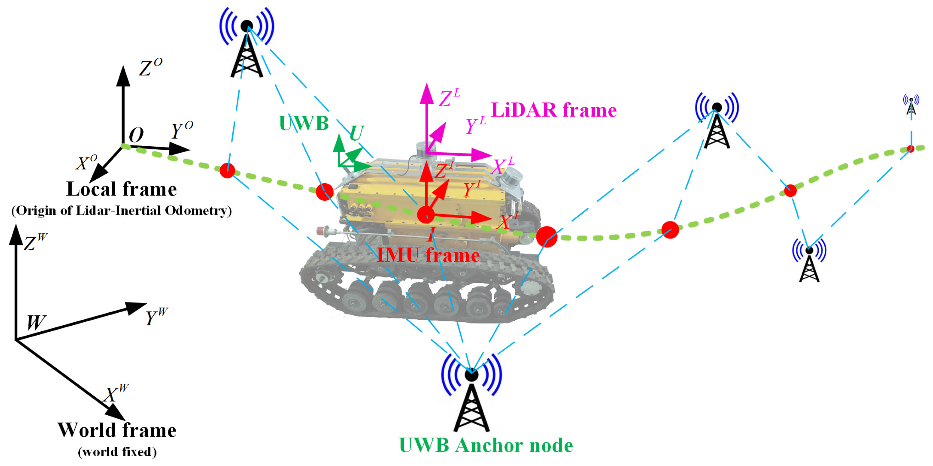


