Abstract
With the ongoing changes in global climate, ocean data play a crucial role in understanding the complex variations in the earth system. These variations pose significant challenges to human efforts in addressing the changes. As a data hub for the satellite geodetic technique, unmanned aerial vehicles (UAVs) instill new vitality into ocean data collection due to their flexibility and mobility. At the same time, the dual-functional radar-communication (DFRC) system is considered a promising technology to empower ubiquitous communication and high-accuracy localization. In this paper, we explore a new fusion of UAV and DFRC to assist data acquisition in the ocean surveillance scenario. The floating buoys transmit uplink data transmission to the UAV with non-orthogonal multiple access (NOMA) and attempt to localize the target cooperatively. With the mobility of the UAV and power control at the buoys, the system throughput and the target localization performance can be improved simultaneously. To balance the communication and sensing performance, a two-objective optimization problem is formulated by jointly optimizing the UAV’s location and buoy’s transmit power to maximize the system throughput and minimize the attainable localization mean-square error. We propose a joint communication and radar-sensing many-objective optimization (CRMOP) algorithm to meliorate the communication and radar-sensing performance simultaneously. Simulation results demonstrate that compared with the baseline, the proposed algorithm achieves superior performance in balancing the system throughput and target localization.
1. Introduction
With the development of marine activity and scientific expeditions, precise and reliable data link communication plays a pivotal role in ocean monitoring [1,2,3]. As an important supplement to the satellite geodesy, unmanned aerial vehicles (UAVs) assisted satellite geodetic techniques to achieve both data acquisition endpoints for receiving sensor-generated data and cooperating with satellites to transmit more refined information [4,5]. There have been a few works researching using UAVs in marine activities as aerial data collectors [6], aerial relays [7], and node complements [8] in integrated air-space networks. Considering the improvement of communication performance, UAV-assisted communication has been regarded as the core technology in the next generation of maritime communication due to its flexibility and mobility, which resolves the long transmission and wide coverage problem in the maritime communication system.
In order to sufficiently exploit the characteristics of the UAV, researchers have conducted extensive investigations on resource management [9,10], channel modeling [11], safety control [12], and performance analysis [13]. The application scenarios of UAV-assisted communication can be summarized into three types, i.e., the UAV serves as a data collector, the cooperative relay and the aerial base station, respectively [14]. Due to maneuverability, UAVs can improve transmission quality by creating line-of-sight (LoS) channels in communication-unfriendly environments. Since most IoT or marine acquisition devices usually have limited transmit power and communication coverage, the flexibility of UAVs can effectively reduce the communication distance and select the optimal location to complete communication tasks. For instance, how to effectively transmit data collected from the sea surface sensor nodes in the ocean monitoring network to the ground base station through UAV cooperative communication is introduced in [15]. In this case, deploying the UAV as a data collection device was devoted to being a profitable and capable scheme. Furthermore, combining the non-orthogonal multiple access (NOMA) and UAV into the wireless network has been regarded as a promising way to promote data collection and spectral efficiency simultaneously. The authors of [16] proposed a new cooperative NOMA scheme for which a UAV transmitted the signals to several base stations (BS) and all of the base stations decoded the message cooperatively. However, a cooperated BS is hard to deploy in an ocean scenario, which makes it not manageable. A UAV-assisted NOMA network where the UAV cooperatively served the ground user to communicate with the base station is investigated in [17]. The NOMA precoding and UAV’s trajectory are jointly optimized to maximize the sum rate. However, such a scheme is not appropriately used in maritime tasks where the base station’s location is usually far from the equipment. In [18], the study of a UAV equipped with a phased-array antenna to receive the signal from the satellite and then transmit the information to the land-based user was investigated, where the trajectory of the UAV and NOMA power was jointly allocated and optimized to achieve a higher energy-efficiency purpose. Unfortunately, considering the complexity of satellite communication systems, using a UAV as a relay to transmit data to ground users will challenge energy efficiency regardless. Furthermore, all of the above research only focuses on UAV-assisted downlink transmission, which means that UAVs are employed to serve ground users or base stations instead of data collection.
Applying the radar sensing function to the sixth-generation communication system opens up possibilities for broadening oceanographic missions [19,20]. Employing the radar function in the UAV-assisted communication system can help the UAV to detect the environment which can avoid potential threats and find the optimal location of the UAV to construct a more stable communication link. Before the dual-functional radar-communication (DFRC) was well studied, most of the works related to UAV-assisted networks were discussed from the perspective of communication and radar separately [21,22,23,24]. However, with the recent development of modern communication technology, combining communication and radar sensing, which is known as DFRC, has attracted extensive attention in the research community [25,26,27]. Based on technology, the communication and radar module could efficiently share the same hardware and obtain the integration gain. In [28], the authors analyzed the advantages of DFRC in self-driving cars to achieve substantial gains in cost, performance, and robustness. The authors of [29] employed the reconfigurable intelligent surface in the DFRC system to improve both the performance of sensing and communication. The sparse antenna array configurations by antenna selection and waveform attend pairing to achieve a higher data rate are investigated in [30]. In addition, the authors of [31] present a hardware prototype of the DFRC system, which utilizes generalized spatial modulation to improve communication performance and reduce the sidelobe level of the transmit beam pattern.
Although the development of DFRC has brought new vitality to the applications of UAVs, the increased complexity induced by the integrated system may lead to more challenges to the optimization design. The traditional method usually optimized the communication performance metrics under the radar constraints or vice versa [32]. Nevertheless, the lack of constraints in one of the specific problems will inevitably affect the final optimization result and the performance trade-off between the two functionalities. Evolutionary multi-objective optimization is beneficial in dealing with such issues. Since the 1990s, the algorithms used to solve the problem with two or three objectives have been proposed [33,34,35] and wildly used in various wild areas such as smelting production measurement systems [36], game map generation [37], and water distribution systems [38]. Some of the typical methods such as the dominance and grid-dominance are driven primarily by concerns about the development of new dominance relations. In contrast, another class of methods such as the non-dominated sorting genetic algorithm II (NSGA-II) focuses on improving diversity to rescue the loss of selection pressure [39,40]. Moreover, there are some methods which find a preferred subset of solutions to shrink the search space and employ dimension reduction to classify the embedded efficient front in the objective neighborhood space.
Among the existing methods, the many-objective optimization algorithm based on dominance and decomposition (MOEA/DD), which integrates the dominance and decomposition approaches, effectively solves the conflicts between convergence, diversity, and computational efficiency [41]. This method proposes a systematic framework to develop a widely spread weight vector in which each vector specifies a unique sub-region in the objective space. Then, it releases the pressure of non-domination and computational efficiency when the number of objectives grows. The constraint consideration is also included in the process of the algorithm, especially when the problem involves a massive number of objectives. Therefore, the MOEA/DD method gives a bright path to solving the multi-objective problem in the DFRC system to optimize the performance of radar and communication simultaneously.
Moreover, under the limited resources of the marine scenario, balancing the advantages of UAVs and DFRC can effectively improve the system’s performance and promote spectral efficiency. However, building a UAV-assisted DFRC data acquisition system to achieve both higher data transmission throughput and radar localization accuracy needs to consider some critical issues, such as the buoy transmit power and the UAV’s location. On the one hand, obtaining the optimal location of the UAV can effectively improve the throughput of the system. On the other hand, according to the construction of different channels, the transmit power of each buoy can be optimized according to the dynamic environment, which ensures the localization accuracy requirement for radar sensing.
1.1. Our Contribution
Against the aforementioned background, we provide a UAV-assisted uplink data collection and target localization network in the ocean surveillance scenario, where the buoys transmit the data to the UAV and localize the target cooperatively. Specifically, data collection between the UAV and buoys is carried out with NOMA and the UAV can be deployed at different locations with its mobility, which achieves higher system throughput under limited communication essentials. The transmit power at the buoys not only affects the data collection but also impacts the target location performance. In order to improve the communication and radar-sensing performance, we formulate a two-objective optimization problem of UAV location and transmit power at the buoys to maximize the system throughput and minimize the Cramer–Rao bound (CRB) of localization simultaneously. We list a CRB-constrained (CRBC) problem to only maximize the system throughput and remark its solution as the baseline to analyze the performance achieved by our design. Simulation results demonstrate the efficiency of our design in balancing the system throughput and target localization performance. The main contributions of this paper are summarized as follows:
- To the best of the authors’ knowledge, this is the first time a UAV-assisted radar-communication network has been investigated where several buoys conduct uplink NOMA data transmission with the UAV while cooperatively sensing the radar target. In order to improve the data collection performance, we exploit the flexible mobility of the UAV and the efficiency of NOMA. Meanwhile, the buoy transmit power is optimized to meliorate the data collection performance and radar target localization simultaneously.
- In order to maximize the system throughput and minimize the CRB of localization, we formulate a two-objective optimization problem of the UAV location and the transmit power of the buoys. To tackle the NP-hard problem, we proposed a joint communication and radar-sensing many-objective optimization (CRMOP) algorithm that achieves a superior balance of data collection and radar target sense.
- In order to facilitate a better comparison with the CRMOP algorithm proposed in this paper, we consider a baseline and propose a CRBC algorithm based on the traditional optimization method where the CRB is regarded as a constraint to maximize the system throughput. Through comprehensive simulations, we demonstrate that our proposed algorithm not only achieves significantly higher throughput but also ensures reliable target localization accuracy.
1.2. Paper Organization
The rest of this paper is organized as follows. The system model and the problem formulation for the UAV-assisted DFRC data collection in the ocean monitoring system are described in Section 2. Section 3 provides the proposed method (CRMOP) to jointly optimize the UAV location and the transmit power of the buoy, followed by the CRBC as a baseline. The simulation results and discussion are shown in Section 4. Finally, we conclude this paper in Section 5. All abbreviations have been presented in Table 1.

Table 1.
List of abbreviations.
2. System Model and Problem Formulation
2.1. System Model
As illustrated in Figure 1, we propose a maritime monitoring data collection system, where a rotary-wing UAV is deployed as a movable access point (AP) to collect data from K single-antenna buoys based on the NOMA principle. Meanwhile, the buoys cooperatively perform radar sensing to localize and track a target through the DFRC signals. The scenario we considered in this paper involves a single data collection process by the UAV and can easily be extended to cover multiple collection processes. All of the buoys are randomly distributed on the sea, and the set of the buoy is denoted as . Without loss of generality, a three-dimensional (3D) Cartesian coordinate system is considered in this paper. To be detailed, the horizontal coordinates of the communication UAV and each buoy are denoted as and , respectively. Although sea clutter, sidelobe, and subspace interference are crucial in marine environments, to present our proposed DFRC system more clearly and simplify the computational steps, we assume that the buoy is relatively stationary at this point [42,43]. Following the assumption in [32], we only consider the UAV’s hovering location and ignore the process of the UAV takeoff and landing. And the UAV is assumed to fly at an unchangeable altitude . Note that the locations of buoys and the UAV are assumed to be almost stable during a short period; thus, the channels remain almost constant, which makes it possible to use the pilot signals to obtain channel state information (CSI). Note that the buoys’ power source is not considered in this system and the transmit power can be optimized when the channel information is known according to the recent development of the energy deployment strategy [44].
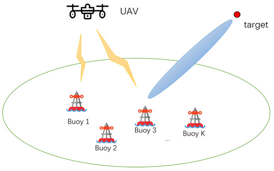
Figure 1.
UAV-assisted DFRC data collection in ocean monitoring system.
In this paper, we assume that all of the UAV–buoy links are referred to the LoS channel model. And the Doppler effect can be perfectly compensated because of the UAV’s mobility [45]. In order to specify the characteristics of the UAV-assisted DFRC ocean monitoring system, the coordinates of all buoys and the CSI of all data links are assumed to be perfectly known by the UAV [46]. Let denote the channel gain between the UAV and the k-th buoy. Then, for , we have
where denotes the channel gain at the reference distance m, denotes the distance between the UAV and the k-th buoy.
As mentioned above, each buoy transmits its signal non-orthogonally to the UAV on the same radio spectrum with controlled transmit power. And the SIC is employed at the UAV to guarantee the experience of distinct channel gains. Toward this end, by assuming that the channel gain of each buoy decreases sequentially, i.e., , we propose to dynamically adjust the transmit power in each buoy. Specifically, through SIC, the signals from stronger data links will be successively decoded while the others with lower channel gains are treated as noise. Therefore, the throughput of each buoy depends on the signal interference from the buoys with lower channel gains. Consequently, the throughput for the k-th buoy can be written as
where is the transmit power of the k-th buoy, is the additive white Gaussian noise (AWGN) power and B is the transmission bandwidth. To guarantee the UAV performs SIC more efficiently, the necessary power constraint for each buoy has to be followed as
where denotes the minimum power difference for SIC. Furthermore, to ensure the uplink transmission requirements of each buoy, the minimum throughput constraint is given by
where is the uplink throughput threshold.
As for the radar sensing, the sensing target with a center of mass is located at [47]. It is assumed that the changes of the target center position and the size observed by the buoys are small relative to the resolution capabilities of the radar function (it is assumed that the position of each buoy is known in advance and the radar sensing-based localization is insensitive to multi-path and weather impacts, which is applicable to localizing the target [48]) which tracks the target’s position and estimates unknown parameters from previous cycles, such as the target’s radar cross-section (RCS). In this premise, by emitting the DFRC signals and then receiving the echoes, the buoys can perform radar detection to sense the location of the target. Since the buoys work in a cooperative method, they can be treated as a distributed MIMO radar. As described in [49], the search cell can be defined as , where I is an integer, and c is the speed of light (all buoys are simultaneous to transmit DFRC signals and receive echo signals by employing a full-duplex transmission implementation. We assume the self-interference is well mitigated according to the existing work [50]). The signal transmitted from buoy and received at buoy can be expressed as
where is the target RCS, is the signal variation due to the path loss effects, denotes the propagation time of the signal transmitted by buoy , reflected by the target, and received by buoy . A group of waveforms is employed, with each waveform possessing a low-pass equivalent of . And is the zero-mean circularly symmetric complex Gaussian noise. As demonstrated in [47], CRB can be used to provide a lower bound on the mean square error (MSE) of asymptotic unbiased parameter estimators in radar sensing, especially when the SNR is sufficiently large, the MSE of the maximum likelihood estimator is close to the CRB. Then, in our considered distributed MIMO radar system, the CRB for the target location estimation can be written as [32]
where is a vector denoting the buoy transmit power, , , , , where the elements are defined as
where and is the distance between the buoy n to the location of the target .
To achieve better localization accuracy, the CRB needs to be as small as possible. After observing Equations (2) and (6), the UAV’s location and buoy transmit power affect the performance of the communication and radar sensing, which should be jointly optimized to obtain a better trade-off. However, conventional methods to deal with such problems generally optimize one performance and treat the others as constraints which can not provide an optimal performance trade-off between the dual functionalities.
2.2. Problem Formulation
In this section, we investigate the multi-objective optimization problem with different design objectives for maximizing the communication throughput and minimizing the CRB for the target location estimation simultaneously. Considering all of the buoys have to be implemented to achieve two individual missions and each object should satisfy the transmit power constraints, as a result, we first formulate the communication sub-problem which maximizes the system throughput under the NOMA protocol given by
where and is the minimum and maximum transmit power of each buoy, constraint (10c) guarantees the effective SIC at the UAV, and constraint (10d) defines the minimum uplink data rate requirements. In order to ensure each buoy sustains a relatively stable working condition, the power of the buoy must be a positive number and have a certain upper threshold. Furthermore, the position of the UAV is limited in such a way that the UAV cannot fly beyond the location of the furthest buoy which is given in (10e) and (10f). Equation (10g) constrains that the minimum distance between the UAV location and the target location.
As for the radar-sensing performance, the optimization sub-problem can be formulated as
where has the same power constraints as in problem (10).
By comparing the sub-problem (P1) and (P2), a non-trivial trade-off design for balancing the communication and radar sensing performance arises in our considered UAV-assisted ocean monitoring system. Both the sub-problems have the same power constraints, while their optimization objectives are not identical, which refer to maximizing the total transmission rate and minimizing the CRB of target location estimation, respectively. Moreover, the variables are tackled in objectives as well as constraints, which makes the problems non-convex and may yield prohibitive complexity. Toward this end, we propose an efficient algorithm to deal with the two conflict objective problem which will be detailed in the next section.
3. Method
In order to resolve the different design objectives, we propose the CRMOP algorithm based on the penalty-based boundary intersection (PBI) approach to combine the original object functions formulated as [41]
where
where is the weighted vector, is the ideal optimal vector with and , is a self-defined penalty indicator which controls the bias of and . Compared to the traditional approach [51], the method employed in (12) balances the convergence and diversity in which is used to assess the convergence of each parameter toward the efficient front and is the measurement of population diversity. We aim to decrease the object value as small as possible so that it can reach the optimal boundary. The proposed algorithm can effectively combine the two objectives and ensure the diversity of the population results, and at the same time has a better performance in dealing with constraints.
3.1. Overall Process of the Proposed Algorithm
The overall process of our proposed algorithm that jointly optimizes the UAV’s location and the transmit power of each buoy to achieve the optimal transmission throughput and the CRB for localization simultaneously is summarized in Algorithm 1. And the details for each stage are given in the following subsections.
| Algorithm 1 Overall Process of the Proposed Algorithm |
|
| Algorithm 2 Initial Parameter Determination | |
| Output: | |
| Intial UAV’s location , buoy transmit power , weight vectors and neighborhood set of weight vectors . | |
| Process: | |
| 1: | Randomly generate the initial parent population and following the uniform distribution. |
| 2: | Use Das and Dennis’s method to generate weight vectors . |
| 3: | while do |
| 4: | Generate M closest neighborhood weight vectors to . |
| 5: | end while |
| 6: | Divide and to several non-domination levels by non-dominated sorting method. |
| 7: | Associate each value in and with unique sub-region. |
| Algorithm 3 Offspring Parameter Generation |
| Output: |
| Offspring solutions and . |
|
3.2. Parameter Initialization
The initial UAV’s location and buoy transmit power are obtained following the process in Algorithm 2. The initial process consists of four parts, i.e., the initialization of parent population and , generation of the weight vectors, the non-domination level processing, and the neighborhood generation, which initialize the parameters utilized for the upcoming stage. To be detailed, the initial values of and are randomly sampled within the corresponding range uniformly. Then, Das and Dennis’s approach is employed to generate the weight vectors [53]. In this step, N points of weight vectors are sampled with a uniform spacing , where U is the number of considerations along each target objective function. It should be pointed out that the choice of U has to be greater than the number of object functions that guarantee our population diversity.
The sub-region in the objective space specified by each weight vector can be defined as
where , is the acute angle between and . The neighborhood of each weight vector consists of M closest weight vectors which are calculated by Euclidean distances. Subsequently, the parameters are divided into several non-domination levels by the non-dominated sorting method, and each value in and is randomly associated with a unique sub-region.
| Algorithm 4 Constraint Operation |
|
3.3. Offspring Parameter Generation
The offspring parameter generation aims to generate offspring solutions based on the initial UAV’s location and buoy transmit power, which contains two main steps, i.e., mating selection and variation operation, as shown in Algorithm 3. The mating selection should choose the parents from the neighborhood as much as possible because each solution is specified by a weight vector and associated with a sub-region. Therefore, the neighborhood solutions can be easily chosen from their sub-regions with the current weight vector. The mating parents are randomly chosen based on the initial UAV’s location and buoy transmit power to avoid any associated solutions in the selected sub-regions. Moreover, according to [54], selecting the mating parents in a low probability from all candidates can enhance the exploration ability. Finally, the selected parent parameter is employed to generate the offspring solutions and based on the method of polynomial mutation and simulated binary crossover.
| Algorithm 5 Update Parent Population of Parameters |
| Output: Parent populations of and . |
|
3.4. Update Parent Population Parameter
Note that before the parent populations are generated, the constraints of the objective problem have to be considered. To deal with this issue, we define the constraint violation value for each user k as
where two parts of the right-hand side are referred from (10c) and (10d), respectively. The operator indicates the absolute value of , and returns 0 otherwise. It is noted that the feasible solution of (16) has to be equal to 0, and the quality of the parameter depends on how much smaller the is. If every value of and are conform to the constraint requirement, the member will be served for the unconstraint update procedure. Otherwise, the infeasible solution will be decided by the and niching scenarios. Obviously, the population diversity depends on the solution associated with an isolated sub-region significantly.
For those values of and which are not conformed to the constraint requirement, there are two scenarios to identify the solutions and .
3.4.1. Case with Only One Non-domination Level
All solutions in and are non-dominated from each other. The density estimation and scalarization functions are employed to obtain the solutions. The density of a sub-region can be estimated since each result is associated with a sub-region. The most crowded sub-region has the largest niche count. However, more than one sub-region may have the same largest niche count. To avoid this scenario, the largest sum of the PBI value is defined as
where is the set of sub-region indicator in which the same largest niche count is included. Then, the worst solutions and in which have the largest PBI value will be eliminated from and given by
3.4.2. Case with More than One Nondomination Level
Since we have to eliminate only one solution from and , the last non-domination level is chosen to process.
Specifically, if the last non-domination level contains only one solution of and , the density of the sub-region has to be investigated first. In this case, if the associated sub-region has more than one solution, and will be eliminated from and . In terms of convergence, better solutions inside of will be contained, and the solutions can not provide further useful information. Otherwise, might not be fully exploited in the object space, which can be treated as the isolated sub-region. and play an important role in population diversity which will be saved to the next round. Then, the worst solutions which are obtained in the most crowded sub-region that are included in the current worst non-domination level are eliminated from , based on the following
If the last non-domination level contains more than one solution. There are also two cases that have to be considered. If more than one solution is related to the most crowded sub-region , the worst solution which has the largest PBI value is eliminated from , according to (18). Otherwise, if every member is associated with an isolated sub-region, the solutions will be saved for the next round and the worst solution is eliminated from , . Once the worst solution is eliminated from and , the non-domination level structure is updated to form the parent population and . Furthermore, if every member in the last nomination level is associated with an isolated sub-region, the worst solution will be eliminated from , .
Considering the infeasible solutions associated with an isolated sub-region is given a second chance to survive in the process. Specifically, the solutions in and which has the largest is identified first. The solutions will be considered the current worst solutions if they are not associated with an isolated sub-region. Otherwise, they will be preserved for later consideration to guarantee population density. And the solution in and which has the second largest solution of (16) will be obtained instead. Whether the solutions are treated as and depends on whether the solutions are associated with an isolated sub-region. Moreover, if every infeasible solution in and is associated with an isolated sub-region, the solutions with the largest will be considered as and and then be eliminated from and .
The update procedure aims to update the -th iteration of parent population of UAV’s location and buoy transmit power to obtain the optimal parameters by generating offspring parameters and . The overall update process is shown in Algorithm 5. Firstly, the sub-region associated with the offspring solutions and is calculated by (15). The hybrid population and are formed by combining with and with , respectively. Then, the non-domination level structure is updated according to [55]. Finally, the -th iteration of parent populations and are generated.
3.5. Convergency and Complexity Analysis
To solve the original problems, we handle two conflict object problems with the help of the CRMOP algorithm based on MOEA/DD to update the solutions until coverage. The convergence of the whole algorithm is influenced by the update process apparently. Since the PBI method acts as the leading role of our proposed algorithms, the objective function is constantly approaching the ideal object value as the iteration processes during the update process which indicates that the algorithm is guaranteed to converge [52]. The complexity of polynomial mutation and SBX in Algorithm 3 is , where D is the number of decision variables. Identifying the ideal point requires a total of computations. As for the update process in Algorithm 5, the non-dominated sorting of a population of size 2N with 2-dimensional objective vectors requires computations [56]. Assuming that the number of solutions in the last non-domination level is L. For each solution, the checking process needs computations. Inspired by the algorithm proposed in [52], the worst complexity of the complexity of one generation approximates . The algorithm proposed in this manuscript provides a theoretical foundation and guidance for localization in practical settings.
3.6. CRBC Optimization (Baseline)
In this subsection, we present a traditional approach to compare the communication and localization performance between our proposed algorithm and the traditional method [32]. An optimization problem is formulated to maximize the system throughput with the given CRBC, which can be expressed as follows
where denotes the given localization accuracy threshold. Noting that problem (20) is a non-convex problem and is extremely difficult to solve directly, we decouple problem (20) into two sub-problems, the UAV location and the power control problems. We first select a proper UAV location by transforming the objective function into a minimization of the sum distance from the UAV to the buoys with respect to the constraints of UAV location [57], which can be written as
Noting that problem (21) is not convex due to the non-convex constraint (21d), we adopt the successive convex optimization technique to obtain the UAV location. The left-hand term in (21d) is convex with respect to and the lower-bound of the convex term can be attained according to the first-order Taylor expansion [46]. Specifically, define as the given point in the r-th iteration and the left hand term in (21d) can be lower bounded as
Then, (21) is transformed into
which is a convex problem and can be easily solved by standard convex optimization solvers such as CVX toolbox [58].
With the obtained UAV location in (23), the system throughput can be maximized by power control at the buoys. We relax the constraint (20g) as in [47] and the power control sub-problem can be given as
We remark that (24) is a convex problem, which can be easily solved.
4. Results and Discussion
In this section, the simulation results are presented to evaluate the performance of our proposed UAV-assisted ocean monitoring radar-communication system. Thanks to [59] for the proposed platform which provides some basic algorithm codes that simplify some of our repetitive work. We investigate the optimal position of the UAV and its impact on the performance of the system under different buoy distribution methods. Employing a UAV as an independent data collector to gather data from the transmitting buoys is a reasonable approach in practical applications and the configuration of four buoys and one UAV is a common deployment setup in practical communication and radar systems [9,12]. To better showcase the superiority of our proposed system without sacrificing generality, and to facilitate future extensions of the proposed system, four buoys are distributed on the sea surface in a two-dimensional area of 1 km × 1 km. The scope of the entire system we have devised aligns with the majority of application scenarios introduced in Section 1 ([6,9,11,16]). Furthermore, it is well suited for deployment and can be easily extended to several working environments. Unless otherwise stated, the default minimum power difference for SIC is set as 2 dB, the bandwidth is set as 50 MHz, the default target location is presented in Location 1, the buoy distribution situation is random, and the maximum buoy transmit power is 18 dBm. Moreover, the UAV is assumed to fly at a constant height. The remaining parameters are summarized in Table 2. To ensure the effectiveness and comparability of the experiments, relevant communication parameters such as AWGN power and UAV altitudes are kept consistent with the [32]. This is carried out to maintain the validity and continuity of the results obtained. In order to enhance the experimental and facilitate accurate comparisons, careful attention is given to aligning these specific parameters with those reported in the relevant paper.
Table 2.
Simulation parameters.
4.1. Nondominated Front Generation
The non-dominated front, also called Pareto Front (PF), is composed of all Pareto-optimal solutions as shown in Figure 2. Thirty points of randomly distributed buoys are selected to generate the experiment result. Considering the problem is a two-objective optimization, each point on the PF does not dominate the other points, which indicates the solutions lie in the PF achieving high performance on communication and radar simultaneously. From Figure 2, we can see that all points are smoothly distributed on the curve with the horizontal axis from to and the vertical axis from bps to bps. It is worth noting that these values are not unique, which indicates that different buoy distributions and numbers or other parameters such as the location of the UAV will result in different final PF values.
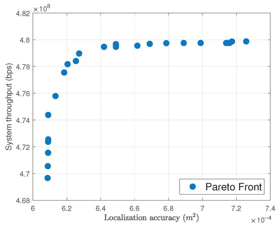
Figure 2.
The non-dominated front obtained by the CRMOP algorithm.
4.2. UAV Optimal Location
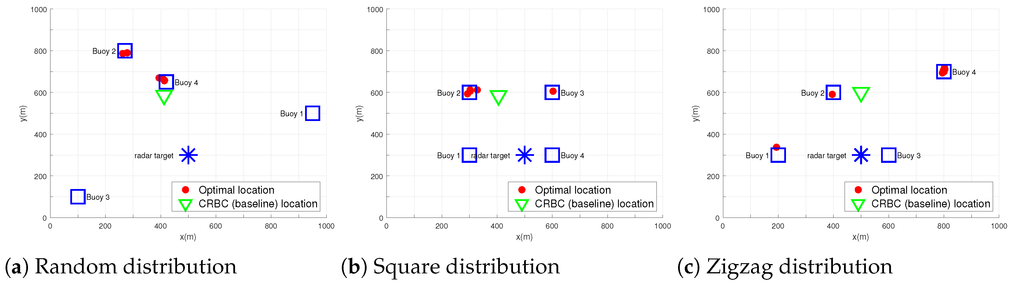
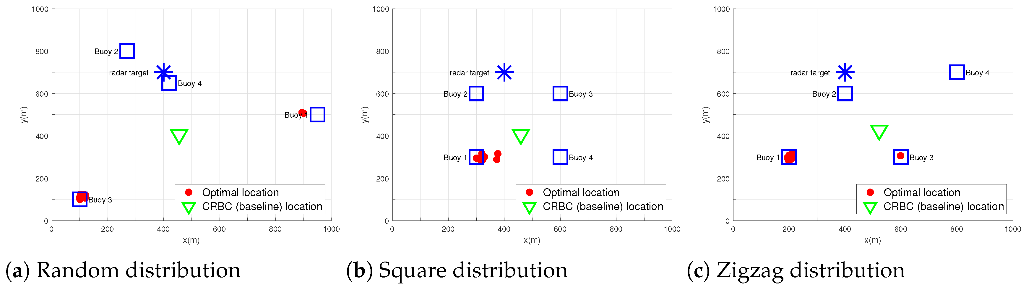
As shown in Figure 3 and Figure 4, we simulate three different buoy distribution situations which are random distribution, square distribution, and zigzag distribution to illustrate the optimal UAV’s location obtained by our proposed algorithm. Since the numerical results obtained from the UAV’s positions on the PF do not dominate each other, we plot all of the optimal positions of the UAV on a single figure. The location of each buoy is marked as a blue square, and the red dot denotes the optimal location obtained by the CRMOP algorithm. The UAV location obtained by the CRBC baseline is marked as a green triangle. As can be seen, different buoy distributions influence the final UAV’s optimal location since both performances of communication and radar are considered. Specifically, according to Figure 3a, when the buoys are randomly distributed on the sea surface, the UAV will choose the location near the second or the fourth buoy as the best reception location. However, when the distribution of buoys has a dedicated pattern, such as square and zigzag distribution, as shown in Figure 3b,c, the locations of the UAV will present different distributions to achieve the optimal performance on radar and data collection at the same time. Moreover, the target location also plays the important role in the UAV’s location optimization process. For example, when the target is located in Location 2 as in Figure 4a shows, the UAV chooses the location near the first or third buoy as the optimal location instead of the second or the fourth in Figure 3a. Due to the optimization process of the UAV’s location being affected by the constraint of the minimum distance between the UAV and the target, the optimal location of the UAV is closely associated with the target location to reach the optimal result. The corresponding object values associated with the parameter are presented in Table 3. In each case, we have chosen two examples for different location areas. From Table 3 and its associated Figure 3 and Figure 4, we can see that there is always a certain distance between the location obtained by the CRBC and the CRMOP algorithm which causes different performances on the system throughput and the achieved CRB for localization. Furthermore, although the power allocated by each buoy has little relationship with the optimal location, the CRMOP algorithm can make our system throughput fluctuate within a certain range without causing a large change in the final result.

Figure 3.
Different buoy distributions with Target Location 1.
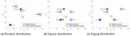
Figure 4.
Different buoy distributions with Target Location 2.
Table 3.
Parameter examples.
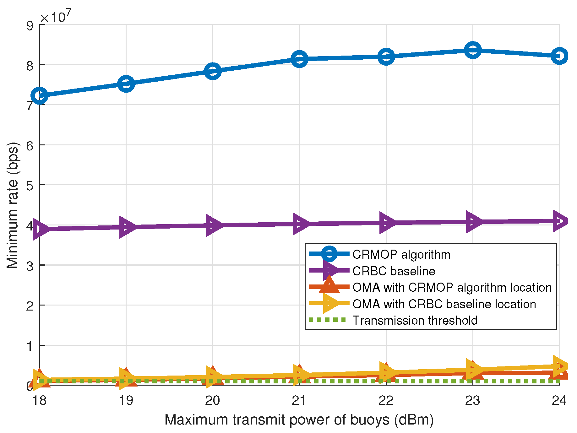
Figure 5 and Figure 6 plot the system throughput under different maximum transmit power of buoys from 18 dBm to 24 dBm. The system throughput and minimum rate of CRBC baseline and orthogonal multiple access (OMA) are compared with our proposed CRMOP algorithm. To better evaluate the impact of the optimized variables on the system, we applied the UAV locations optimized by the CRMOP algorithm and CRBC baseline separately to the OMA protocol, which allows us to comprehensively assess the effectiveness of the optimizations and their impact on the overall performance of the system [32].
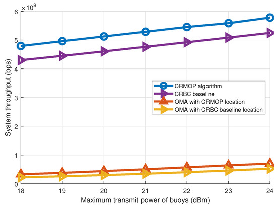
Figure 5.
System throughput under different maximum buoy transmit power.
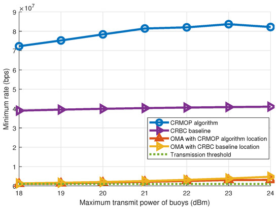
Figure 6.
Minimum rate under different maximum buoy transmit power.
It can be observed that the maximum transmit power increment improves the throughput for all cases. No matter the minimum rate or system throughput, the performance of our proposed algorithm and CRBC baseline is much higher than that of the OMA protocol, which illustrates the advantage of applying NOMA in the system. Moreover, our proposed CRMOP algorithm has better performance than the CRBC baseline which reveals the superiority of our proposed algorithm for solving the UAV-assisted ocean monitoring problem. The system throughput of the OMA protocol at different UAV locations is shown in Figure 5, which demonstrates that the proposed algorithm yields better results than the traditional method when the UAV is located in the location optimized by our algorithm.
4.3. Performance Comparisons between CRMOP Algorithm and the CRBS Baseline
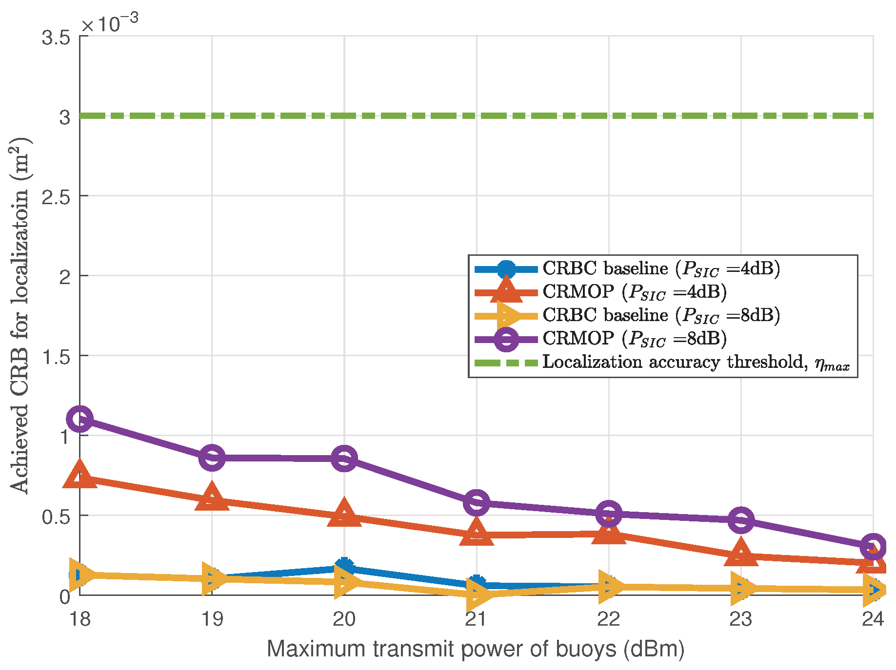
Finally, we compare the proposed CRMOP algorithm and CRBC baseline in terms of achieved CRB for localization and system throughput under the same SIC constraint. Figure 7 and Figure 8 show the system throughput with the two algorithms in the case of 4 dB and 8 dB. When is small, the power of the buoy has more flexibility for data transmission so that the system will have a higher throughput. As for the CRBC baseline, changing the does not impact the system’s performance significantly. Moreover, it has been consistently observed that no matter what the is, the CRMOP algorithm has better performance than the CRBC baseline.
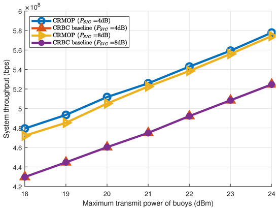
Figure 7.
System throughput under different maximum buoy transmit power.
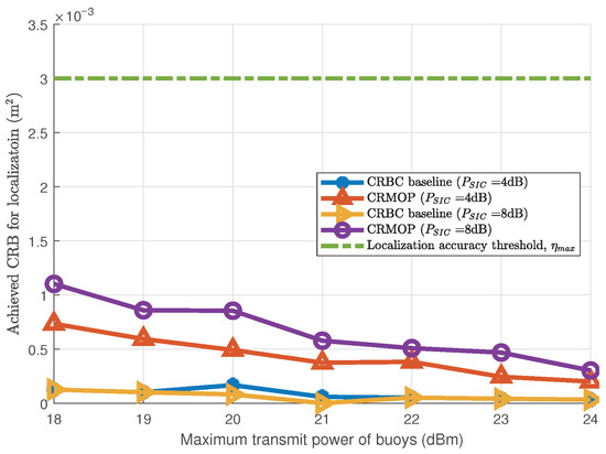
Figure 8.
Achieved CRB for localization under different maximum buoy transmit power.
For the achieved CRB for localization, it is clear that all cases are below the green dotted line which indicates that both algorithms are better than the preset threshold. The flexibility of the buoy’s power for radar functions increases as the is incremented, resulting in a lower achieved CRB for system localization. Another interesting phenomenon is that the CRMOP algorithm exhibits superior throughput compared to the CRBC baseline while the latter demonstrates better radar accuracy, despite both meeting the threshold requirements for radar performance. Moreover, the change of has little effect on both the system throughput and achieved CRB for localization of the CRBC baseline. This is because when other parameters are fixed and meets the requirements of NOMA, the distribution of the UAV’s position and power can converge to a certain range to reach the optimal value of the objective function.
5. Conclusions
In this paper, we investigated a UAV-assisted DFRC system in the ocean monitoring scenario to simultaneously realize data collection and target localization. To maximize the communication throughput while minimizing the CRB of localization at the same time, we formulate a two-objective optimization problem under constraints of buoy transmit power threshold and the available UAV’s location. A joint communication and radar sensing many-objective optimization algorithm is proposed to solve this problem. Numerical results revealed the superiority of our proposed algorithm in the ocean monitoring data collection system which significantly improves both the network throughput and the localization accuracy. This proposed design can be used for complex marine activities that require multiple tasks to be performed simultaneously and will improve the efficiency and performance of different tasks. However, in real-world scenarios, controlling all factors becomes more challenging due to external influences, unpredictable events, and limitations in experimental setup. In the future, we will consider additionally exploring the impact of other variables, such as UAV operation or wireless environments, as well as the effects of energy consumption and multi-target detection capability on the DFRC system in marine scenarios.
Author Contributions
Conceptualization, Y.L. and F.H.; methodology, Y.L.; software, Y.L.; validation, Y.L., F.H. and M.C.; formal analysis, H.J.; investigation, H.Z.; resources, S.Z.; data curation, S.Z.; writing—original draft preparation, Y.L.; writing—review and editing, M.C.; visualization, S.Z.; supervision, S.Z.; project administration, H.J.; funding acquisition, S.Z. All authors have read and agreed to the published version of the manuscript.
Funding
This work was supported in part by National Key R&D Program of China 2019YFB2102300 and 2019YFB2102301, in part by National Natural Science Foundation of China under Grant 61936014, in part by National Natural Science Foundation of China under Grant 62201388, in part by Shanghai Municipal Science and Technology Major Project No. 2021SHZDZX0100, in part by Shanghai Science and Technology Innovation Action Plan Project 22511105300, in part by Natural Science Foundation of Shanghai: 22ZR1463400, and in part by Fundamental Research Funds for the Central Universities.
Institutional Review Board Statement
Not applicable.
Informed Consent Statement
Not applicable.
Data Availability Statement
Data is unavailable due to privacy restrictions.
Conflicts of Interest
The authors declare no conflict of interest.
References
- Zhu, J.; Song, Y.; Jiang, N.; Xie, Z.; Fan, C.; Huang, X. Enhanced Doppler Resolution and Sidelobe Suppression Performance for Golay Complementary Waveforms. Remote Sens. 2023, 15, 2452. [Google Scholar] [CrossRef]
- Liu, H.; Li, J.; Meng, X.; Zhou, B.; Fang, G.; Spencer, B.F. Discrimination Between Dry and Water Ices by Full Polarimetric Radar: Implications for China’s First Martian Exploration. IEEE Trans. Geosci. Remote Sens. 2023, 61, 5100111. [Google Scholar] [CrossRef]
- Mao, Y.; Sun, R.; Wang, J.; Cheng, Q.; Kiong, L.C.; Ochieng, W.Y. New time-differenced carrier phase approach to GNSS/INS integration. GPS Solut. 2022, 26, 122. [Google Scholar] [CrossRef]
- Akyildiz, I.F.; Kak, A.; Nie, S. 6G and Beyond: The Future of Wireless Communications Systems. IEEE Access 2020, 8, 133995–134030. [Google Scholar] [CrossRef]
- Jiang, H.; Mukherjee, M.; Zhou, J.; Lloret, J. Channel Modeling and Characteristics for 6G Wireless Communications. IEEE Netw. 2021, 35, 296–303. [Google Scholar] [CrossRef]
- Wang, Q.; Dai, H.N.; Wang, Q.; Shukla, M.K.; Zhang, W.; Soares, C.G. On Connectivity of UAV-Assisted Data Acquisition for Underwater Internet of Things. IEEE Internet Things J. 2020, 7, 5371–5385. [Google Scholar] [CrossRef]
- Wang, X.; Fu, L.; Chen, N.; Sun, R.; Luan, T.H.; Quan, W.; Aldubaikhy, K. Joint Flying Relay Location and Routing Optimization for 6G UAV-IoT Networks: A Graph Neural Network-Based Approach. Remote Sens. 2022, 14, 4377. [Google Scholar] [CrossRef]
- Huo, Y.; Dong, X.; Beatty, S. Cellular Communications in Ocean Waves for Maritime Internet of Things. IEEE Internet Things J. 2020, 7, 9965–9979. [Google Scholar] [CrossRef]
- Zeng, Y.; Xu, J.; Zhang, R. Rotary-Wing UAV Enabled Wireless Network: Trajectory Design and Resource Allocation. In Proceedings of the 2018 IEEE Global Communications Conference (GLOBECOM), Abu Dhabi, Saudi Arabia, 9–13 December 2018. [Google Scholar]
- Zheng, Q.; Zhao, P.; Li, Y.; Wang, H.; Yang, Y. Spectrum interference-based two-level data augmentation method in deep learning for automatic modulation classification. Neural Comput. Appl. 2021, 33, 7723–7745. [Google Scholar] [CrossRef]
- Lian, Z.; Ji, P.; Wang, Y.; Su, Y.; Jin, B.; Zhang, Z.; Xie, Z.; Li, S. Geometry-Based UAV-MIMO Channel Modeling Assisted by Intelligent Reflecting Surface. IEEE Trans. Veh. Technol. 2022, 71, 6698–6703. [Google Scholar] [CrossRef]
- Wang, W.; Li, X.; Zhang, M.; Cumanan, K.; Kwan Ng, D.W.; Zhang, G.; Tang, J.; Dobre, O.A. Energy-Constrained UAV-Assisted Secure Communications With Position Optimization and Cooperative Jamming. IEEE Trans. Commun. 2020, 68, 4476–4489. [Google Scholar] [CrossRef]
- Xie, L.; Xu, J.; Zhang, R. Throughput Maximization for UAV-Enabled Wireless Powered Communication Networks. IEEE Internet Things J. 2019, 6, 1690–1703. [Google Scholar] [CrossRef]
- Mozaffari, M.; Saad, W.; Bennis, M.; Nam, Y.H.; Debbah, M. A Tutorial on UAVs for Wireless Networks: Applications, Challenges, and Open Problems. IEEE Commun. Surv. Tutorials 2019, 21, 2334–2360. [Google Scholar] [CrossRef]
- Ma, R.; Wang, R.; Liu, G.; Chen, H.H.; Qin, Z. UAV-Assisted Data Collection for Ocean Monitoring Networks. IEEE Netw. 2020, 34, 250–258. [Google Scholar] [CrossRef]
- Mei, W.; Zhang, R. Uplink Cooperative NOMA for Cellular-Connected UAV. IEEE J. Sel. Top. Signal Process. 2019, 13, 644–656. [Google Scholar] [CrossRef]
- Zhao, N.; Pang, X.; Li, Z.; Chen, Y.; Li, F.; Ding, Z.; Alouini, M.S. Joint Trajectory and Precoding Optimization for UAV-Assisted NOMA Networks. IEEE Trans. Commun. 2019, 67, 3723–3735. [Google Scholar] [CrossRef]
- Wang, N.; Li, F.; Chen, D.; Liu, L.; Bao, Z. NOMA-Based Energy-Efficiency Optimization for UAV Enabled Space-Air-Ground Integrated Relay Networks. IEEE Trans. Veh. Technol. 2022, 71, 4129–4141. [Google Scholar] [CrossRef]
- De Lima, C.; Belot, D.; Berkvens, R.; Bourdoux, A.; Dardari, D.; Guillaud, M.; Isomursu, M.; Lohan, E.S.; Miao, Y.; Barreto, A.N.; et al. Convergent Communication, Sensing and Localization in 6G Systems: An Overview of Technologies, Opportunities and Challenges. IEEE Access 2021, 9, 26902–26925. [Google Scholar] [CrossRef]
- Qian, L.; Zheng, Y.; Li, L.; Ma, Y.; Zhou, C.; Zhang, D. A New Method of Inland Water Ship Trajectory Prediction Based on Long Short-Term Memory Network Optimized by Genetic Algorithm. Appl. Sci. 2022, 12, 4073. [Google Scholar] [CrossRef]
- Zhang, J.; Liang, F.; Li, B.; Yang, Z.; Wu, Y.; Zhu, H. Placement optimization of caching UAV-assisted mobile relay maritime communication. China Commun. 2020, 17, 209–219. [Google Scholar] [CrossRef]
- Ma, Z.; Ai, B.; He, R.; Wang, G.; Niu, Y.; Yang, M.; Wang, J.; Li, Y.; Zhong, Z. Impact of UAV Rotation on MIMO Channel Characterization for Air-to-Ground Communication Systems. IEEE Trans. Veh. Technol. 2020, 69, 12418–12431. [Google Scholar] [CrossRef]
- Liu, Y.; Wang, C.X.; Chang, H.; He, Y.; Bian, J. A Novel Non-Stationary 6G UAV Channel Model for Maritime Communications. IEEE J. Sel. Areas Commun. 2021, 39, 2992–3005. [Google Scholar] [CrossRef]
- Yin, J.; Hoogeboom, P.; Unal, C.; Russchenberg, H.; van der Zwan, F.; Oudejans, E. UAV-Aided Weather Radar Calibration. IEEE Trans. Geosci. Remote Sens. 2019, 57, 10362–10375. [Google Scholar] [CrossRef]
- Liu, F.; Masouros, C.; Petropulu, A.P.; Griffiths, H.; Hanzo, L. Joint Radar and Communication Design: Applications, State-of-the-Art, and the Road Ahead. IEEE Trans. Commun. 2020, 68, 3834–3862. [Google Scholar] [CrossRef]
- Zhang, J.A.; Liu, F.; Masouros, C.; Heath, R.W.; Feng, Z.; Zheng, L.; Petropulu, A. An Overview of Signal Processing Techniques for Joint Communication and Radar Sensing. IEEE J. Sel. Top. Signal Process. 2021, 15, 1295–1315. [Google Scholar] [CrossRef]
- Wen, C.; Huang, Y.; Zheng, L.; Liu, W.; Davidson, T.N. Transmit Waveform Design for Dual-Function Radar-Communication Systems via Hybrid Linear-Nonlinear Precoding. IEEE Trans. Signal Process. 2023, 71, 2130–2145. [Google Scholar] [CrossRef]
- Ma, D.; Shlezinger, N.; Huang, T.; Liu, Y.; Eldar, Y.C. Joint Radar-Communication Strategies for Autonomous Vehicles: Combining Two Key Automotive Technologies. IEEE Signal Process. Mag. 2020, 37, 85–97. [Google Scholar] [CrossRef]
- Liu, R.; Li, M.; Liu, Y.; Wu, Q.; Liu, Q. Joint Transmit Waveform and Passive Beamforming Design for RIS-Aided DFRC Systems. IEEE J. Sel. Top. Signal Process. 2022, 16, 995–1010. [Google Scholar] [CrossRef]
- Wang, X.; Hassanien, A.; Amin, M.G. Dual-Function MIMO Radar Communications System Design Via Sparse Array Optimization. IEEE Trans. Aerosp. Electron. Syst. 2019, 55, 1213–1226. [Google Scholar] [CrossRef]
- Ma, D.; Shlezinger, N.; Huang, T.; Shavit, Y.; Namer, M.; Liu, Y.; Eldar, Y.C. Spatial Modulation for Joint Radar-Communications Systems: Design, Analysis, and Hardware Prototype. IEEE Trans. Veh. Technol. 2021, 70, 2283–2298. [Google Scholar] [CrossRef]
- Wang, X.; Fei, Z.; Zhang, J.A.; Huang, J.; Yuan, J. Constrained Utility Maximization in Dual-Functional Radar-Communication Multi-UAV Networks. IEEE Trans. Commun. 2021, 69, 2660–2672. [Google Scholar] [CrossRef]
- Knowles, J.D.; Corne, D.W. Approximating the Nondominated Front Using the Pareto Archived Evolution Strategy. Evol. Comput. 2000, 8, 149–172. [Google Scholar] [CrossRef]
- Zitzler, E.; Thiele, L. Multiobjective evolutionary algorithms: A comparative case study and the strength Pareto approach. IEEE Trans. Evol. Comput. 1999, 3, 257–271. [Google Scholar] [CrossRef]
- Zitzler, E.; Thiele, L.; Laumanns, M.; Fonseca, C.; da Fonseca, V. Performance assessment of multiobjective optimizers: An analysis and review. IEEE Trans. Evol. Comput. 2003, 7, 117–132. [Google Scholar] [CrossRef]
- Zhang, H.; Zhao, J.; Leung, H.; Wang, W. Adaptive Weighted Optimization Framework for Multiobjective Long-Term Planning of Concentrate Ingredients in Copper Industry. IEEE Trans. Instrum. Meas. 2022, 71, 2508913. [Google Scholar] [CrossRef]
- Ma, L.; Cheng, S.; Shi, M.; Guo, Y. Angle-Based Multi-Objective Evolutionary Algorithm Based On Pruning-Power Indicator for Game Map Generation. IEEE Trans. Emerg. Top. Comput. Intell. 2022, 6, 341–354. [Google Scholar] [CrossRef]
- Wang, Q.; Liu, S.; Wang, H.; Savić, D.A. Multi-Objective Cuckoo Search for the Optimal Design of Water Distribution Systems. In Civil Engineering and Urban Planning; ASCE: Reston, VA, USA, 2012. [Google Scholar]
- Wagner, T.; Beume, N.; Naujoks, B. Pareto-, Aggregation-, and Indicator-Based Methods in Many-Objective Optimization; Springer: Berlin/Heidelberg, Germany, 2006. [Google Scholar]
- Deb, K.; Pratap, A.; Agarwal, S.; Meyarivan, T. A fast and elitist multiobjective genetic algorithm: NSGA-II. IEEE Trans. Evol. Comput. 2002, 6, 182–197. [Google Scholar] [CrossRef]
- Li, K.; Deb, K.; Zhang, Q.; Kwong, S. An Evolutionary Many-Objective Optimization Algorithm Based on Dominance and Decomposition. IEEE Trans. Evol. Comput. 2015, 19, 694–716. [Google Scholar] [CrossRef]
- Zhu, J.; Wang, X.; Huang, X.; Suvorova, S.; Moran, B. Detection of moving targets in sea clutter using complementary waveforms. Signal Process. 2018, 146, 15–21. [Google Scholar] [CrossRef]
- Liu, W.; Liu, J.; Liu, T.; Chen, H.; Wang, Y.L. Detector Design and Performance Analysis for Target Detection in Subspace Interference. IEEE Signal Process. Lett. 2023, 30, 618–622. [Google Scholar] [CrossRef]
- Ruan, Y.; Jiang, L.; Li, Y.; Zhang, R. Energy-Efficient Power Control for Cognitive Satellite-Terrestrial Networks With Outdated CSI. IEEE Syst. J. 2021, 15, 1329–1332. [Google Scholar] [CrossRef]
- Wu, Q.; Zeng, Y.; Zhang, R. Joint Trajectory and Communication Design for Multi-UAV Enabled Wireless Networks. IEEE Trans. Wirel. Commun. 2018, 17, 2109–2121. [Google Scholar] [CrossRef]
- Liu, Y.; Han, F.; Zhao, S. Flexible and Reliable Multiuser SWIPT IoT Network Enhanced by UAV-Mounted Intelligent Reflecting Surface. IEEE Trans. Reliab. 2022, 71, 1092–1103. [Google Scholar] [CrossRef]
- Godrich, H.; Petropulu, A.P.; Poor, H.V. Power Allocation Strategies for Target Localization in Distributed Multiple-Radar Architectures. IEEE Trans. Signal Process. 2011, 59, 3226–3240. [Google Scholar] [CrossRef]
- Guerra, A.; Dardari, D.; Djuric, P.M. Dynamic Radar Networks of UAVs: A Tutorial Overview and Tracking Performance Comparison With Terrestrial Radar Networks. IEEE Veh. Technol. Mag. 2020, 15, 113–120. [Google Scholar] [CrossRef]
- Meikle, H. Modern Radar Systems; Artech House: London, UK, 2008. [Google Scholar]
- Hassani, S.A.; Guevara, A.; Parashar, K.; Bourdoux, A.; van Liempd, B.; Pollin, S. An In-Band Full-Duplex Transceiver for Simultaneous Communication and Environmental Sensing. In Proceedings of the 2018 52nd Asilomar Conference on Signals, Systems, and Computers, Pacific Grove, CA, USA, 28–31 October 2018; pp. 1389–1394. [Google Scholar] [CrossRef]
- Miettinen, K. Nonlinear Multiobjective Optimization; Springer: Berlin/Heidelberg, Germany, 1998. [Google Scholar]
- Deb, K.; Jain, H. An Evolutionary Many-Objective Optimization Algorithm Using Reference-Point-Based Nondominated Sorting Approach, Part I: Solving Problems With Box Constraints. IEEE Trans. Evol. Comput. 2014, 18, 577–601. [Google Scholar] [CrossRef]
- Das, I.; Dennis, J.E. Normal-Boundary Intersection: A New Method for Generating the Pareto Surface in Nonlinear Multicriteria Optimization Problems. Siam J. Optim. 1996, 8, 631–657. [Google Scholar] [CrossRef]
- Li, H.; Zhang, Q. Multiobjective Optimization Problems With Complicated Pareto Sets, MOEA/D and NSGA-II. IEEE Trans. Evol. Comput. 2009, 13, 284–302. [Google Scholar] [CrossRef]
- Li, K.; Deb, K.; Zhang, Q.; Zhang, Q. Efficient Nondomination Level Update Method for Steady-State Evolutionary Multiobjective Optimization. IEEE Trans. Cybern. 2017, 47, 2838–2849. [Google Scholar] [CrossRef]
- Yuan, Y.; Xu, H.; Wang, B.; Yao, X. A New Dominance Relation-Based Evolutionary Algorithm for Many-Objective Optimization. IEEE Trans. Evol. Comput. 2016, 20, 16–37. [Google Scholar] [CrossRef]
- Liu, X.; Wang, J.; Zhao, N.; Chen, Y.; Zhang, S.; Ding, Z.; Yu, F.R. Placement and Power Allocation for NOMA-UAV Networks. IEEE Wirel. Commun. Lett. 2019, 8, 965–968. [Google Scholar] [CrossRef]
- Grant, M.; Boyd, S. Graph implementations for nonsmooth convex programs. In Recent Advances in Learning and Control; Blondel, V., Boyd, S., Kimura, H., Eds.; Lecture Notes in Control and Information Sciences; Springer: Berlin/Heidelberg, Germany, 2008; pp. 95–110. Available online: https://web.stanford.edu/~boyd/papers/graph_dcp.html (accessed on 22 June 2023).
- Tian, Y.; Cheng, R.; Zhang, X.; Jin, Y. PlatEMO: A MATLAB platform for evolutionary multi-objective optimization. IEEE Comput. Intell. Mag. 2017, 12, 73–87. [Google Scholar] [CrossRef]


Disclaimer/Publisher’s Note: The statements, opinions and data contained in all publications are solely those of the individual author(s) and contributor(s) and not of MDPI and/or the editor(s). MDPI and/or the editor(s) disclaim responsibility for any injury to people or property resulting from any ideas, methods, instructions or products referred to in the content. |
© 2023 by the authors. Licensee MDPI, Basel, Switzerland. This article is an open access article distributed under the terms and conditions of the Creative Commons Attribution (CC BY) license (https://creativecommons.org/licenses/by/4.0/).