Abstract
Parcel detection and boundary delineation play an important role in numerous remote sensing applications, such as yield estimation, crop type classification, and farmland management systems. Consequently, achieving accurate boundary delineation remains a prominent research area within remote sensing literature. In this study, we propose a straightforward yet highly effective method for boundary delineation that leverages frequency attention to enhance the precision of boundary detection. Our approach, named Frequency Attention U-Net (FAUNet), builds upon the foundational and successful U-Net architecture by incorporating a frequency-based attention gate to enhance edge detection performance. Unlike many similar boundary delineation methods that employ three segmentation masks, our network employs only two, resulting in a more streamlined post-processing workflow. The essence of frequency attention lies in the integration of a frequency gate utilizing a high-pass filter. This high-pass filter output accentuates the critical high-frequency components within feature maps, thereby significantly improves edge detection performance. Comparative evaluation of FAUNet against alternative models demonstrates its superiority across various pixel-based and object-based metrics. Notably, FAUNet achieves a pixel-based precision, F1 score, and IoU of 0.9047, 0.8692, and 0.7739, respectively. In terms of object-based metrics, FAUNet demonstrates minimal over-segmentation (OS) and under-segmentation (US) errors, with values of 0.0341 and 0.1390, respectively.
1. Introduction
Parcel boundary delineation refers to the precise identification and marking of the specific boundaries of individual land plots or parcels using remote sensing data. This task holds significant importance in various remote sensing applications, especially within the agricultural sector. For instance, Matton et al. argued that methods utilizing boundaries and treating parcels as cohesive objects rather than fragmented pixels obtain better results in estimating crop yields [1]. Belgiu and Csillik asserted that the same point is valid when it comes to crop classification. They posited that utilizing parcel boundaries in such a manner leads to enhanced classification outcomes [2]. Moreover, Wang et al. argued that parcel-based rice mapping is more effective than its pixel-based counterpart [3]. Furthermore, a study by Yu et al. demonstrated the pivotal role parcel boundaries play in enhancing certain agricultural management systems, showcasing the benefits of accurate delineation [4]. Similarly, many other researchers have used parcel boundaries as an essential step for their crop-mapping schemes, as shown in the works of Chen et al. [5], Li et al. [6].
Before deep learning, the primary methods for boundary delineation relied on edge detection techniques. For instance, Graesser and Ramankutty utilized multi-spectral and multi-temporal edge extraction combined with histogram equalization for unsupervised boundary delineation [7]. Furthermore, Fetai et al. grounded their boundary delineation strategy on the edges derived from the Sobel operator, an edge detection filter [8]. Another study capitalized on both multi-temporal and multi-spectral data to craft and refine closed parcel boundaries. This was achieved by harnessing the outcomes of an edge extraction algorithm, as detailed by Cheng et al. [9].
Recently, deep learning has become a preferred method for boundary delineation in remote sensing, U-Net architecture in particular. One of the first major works in this field is that of Xia et al. [10], who fine-tuned U-Net models to delineate field boundaries, obtaining better results than classical methods. Later on, Garcia-Pedrero et al. [11] applied the same architecture to vineyard boundaries, reporting a better performance than classical methods. Diakogiannis et al. [12] made modifications to the ResUNet architecture, leading to the introduction of ResUNet-a. In this version, they adjusted the loss function and network framework. These changes improved the accuracy of boundary delineation for various remote sensing classes. Going further, the research of Waldner and Diakogiannis [13] addressed the specific task of parcel boundary delineation by integrating three masks: edge, extent, and distance. Their innovative loss function, based on the harmonic mean of the Dice losses for these masks combined with optimization and the watershed method in post-processing, resulted in boundaries of superior accuracy and completeness, achieving an F1 score of 0.89 on their study area. Other researchers have also made contributions to boundary delineation using remote sensing data. Zhang et al. devised a method for Sentinel 2 data, using the potential of a residual U-Net architecture [14]. This method focused on increasing the precision of automated boundary extraction from Sentinel 2 images by using a recurrent U-Net architecture and achieved a F1 score of 0.86 on the chosen study area in China. Waldner et al. also synergized the ResUNet-a with the FracTAL architecture in order to solve large-scale boundary delineation challenges, which claimed to obtain an overall accuracy of 0.87 in pixel-based metrics [15]. Notably, Jong et al. brought an opposing training angle aimed to augment the efficacy of residual U-Net models in the delineation process and increased the performance of ResUNet from 0.75 to 0.88 on their proprietary dataset [16]. Expanding upon the landscape of advancements, Lu and colleagues introduced the Dual Attention and Scale Fusion Network (DASFNet) for high-resolution remote sensing imagery in their publication [17]. DASFNet’s core strength resides in its dual attention mechanism and multi-scale feature fusion module, which enable the model to capture contextual information and integrate features of diverse scales, achieving a 0.9 F1 score on a dataset collected in South Xinjiang, China. Moreover, Xu et al. proposed a unique combination of semantic and edge detection within a cascaded multi-task framework. Their architecture fused a refinement network with fixed-edge local connectivity to ensure robust boundary delineation on high-resolution images, reporting an F1 score of 0.86 [18]. In another work, Long et al. introduced the lightweight multi-task network BsiNet, employing a singular encoder–decoder mechanism. This approach was very successful while maintaining high efficiency standards [19]. Li et al. proposed the semantic edge-aware multi-task neural network SEANet, which achieved an F1 score of 0.85 on a benchmark dataset. The network is made of two main components: PRoI (parcel region of interest) and PEoI (parcel edge of interest) for feature extraction. The PRoI component depends on an encoder–decoder setup for its functionality. In contrast, PEoI focuses on high-level image features. Complementing this structure, a novel multi-task loss function is utilized, specifically designed to factor in uncertainties during the training phase [20].
Building on prior research, we present a novel multi-task segmentation architecture based on the widely-recognized U-Net model. Our approach is centered around the integration of two separate multi-task segmentation masks, a commonly employed strategy in parcel boundary delineation. Furthermore, to enhance the precision of the edge mask and increase the overall segmentation accuracy, we introduce a novel frequency-based attention gate. This gate strategically channels the model’s attention towards high-frequency elements, promoting enhanced segmentation precision and accuracy in the derived results. While our experimental validation shows a clear improvement in accuracy compared to state-of-the-art methods, the simultaneous reduction in required post-processing masks and the model’s relative simplicity sets our work apart from others. The paper is organized as follows: Section 2 expands on some related works; Section 3 introduces the frequency attention gate, frequency attention U-Net (FAUNet), and the post-processing approach; Section 4 lays out the comparative results; and a detailed discussion about the results, limitations of the method, and possible future directions is given in Section 5.
2. Related Work
The field of remote sensing and image analysis has seen important advancements. Multitasking segmentation, exemplified by ResUNet-a, has improved boundary delineation precision. Additionally, attention mechanisms in deep learning have gained prominence for selective focus in different tasks. Our research introduces a novel approach, using high-pass filters to enhance edge detection in boundary delineation. This reduces reliance on the distance mask, making boundary delineation more efficient and precise. The upcoming sections will delve into the models that served as the foundation for our research, including the multitasking segmentation of ResUNet-a and the concept of attention gates and their applications.
2.1. Boundary Delineation as Multitasking Segmentation
Among the various architectures proposed for parcel boundary segmentation, ResUNet-a has emerged as a promising approach, surpassing the state-of-the-art models of its time [13]. ResUNet-a combines several essential components to enhance its segmentation capabilities, making it a robust and effective model. At the core of ResUNet-a lies the U-Net architecture, featuring an encoder and a decoder. The encoder efficiently compresses high-dimensional input images, while the decoder upscales the encoded features, precisely localizing objects of interest. This dual-pathway design facilitates contextual understanding and accurate segmentation [21]. To address the challenges of vanishing and exploding gradients, ResUNet-a incorporates residual blocks. These blocks utilize skip connections to improve information flow between layers, thereby mitigating gradient-related issues [22]. In addition, the model adopts atrous convolutions with multiple parallel branches, each with varying dilation rates. Atrous convolutions significantly increase the receptive field, allowing the model to capture broader contextual information [23]. Further enhancing its contextual awareness, ResUNet-a employs the Pyramid Scene Parsing Pooling (PSPPooling) layer [24]. By applying maximum pooling at different scales, the PSPPooling layer effectively captures dominant contextual features across the image, contributing to improved segmentation results.
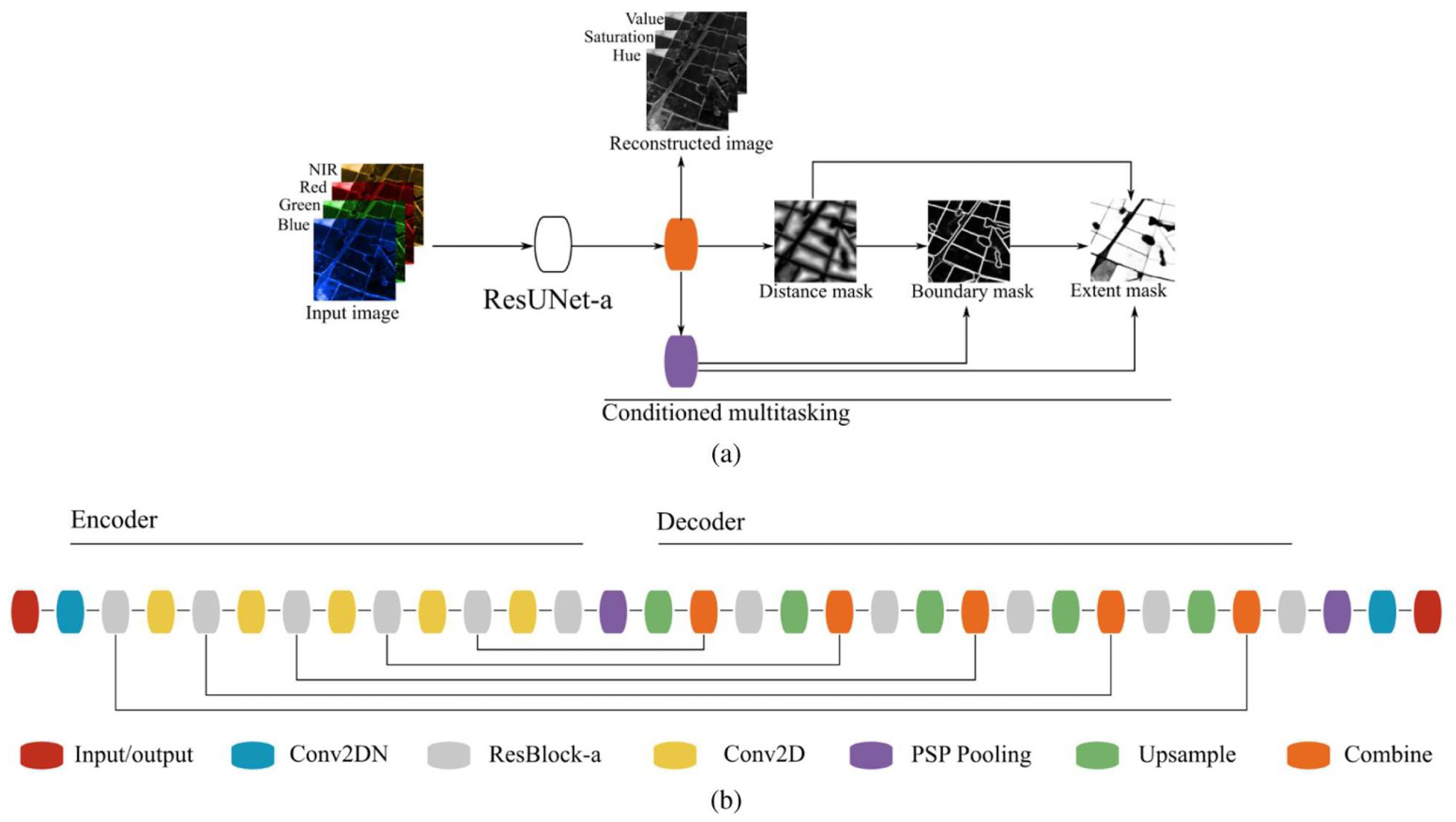
Despite all of the state-of-the-art deep learning approaches employed in ResUNet-a, the most important and distinct aspect remains its conditioned multitasking approach. As seen in Figure 1 the model generates four output layers simultaneously: the extent mask, the boundary mask (we refer to it as the edge mask in our work), the distance mask, and a reconstruction of the original image. At the output layer, the first and last layers of the U-Net are combined. The initial output is the distance mask, which is created without using any PSPPooling. Then, to generate the boundary mask, the distance transformation is combined with the final U-Net layer using PSPPooling. The distance and boundary masks are merged with the output features to create the extent mask. Additionally, a parallel fourth layer reconstructs the original input image, aiding to create a reduction in model variability [12]. The use of multitasking, where the neural network is trained to predict multiple related outputs simultaneously, enhances the quality of boundary predictions and contributes to the generation of closed contours. By leveraging the correlation between outputs like boundary, distance, and extent, the network can benefit from the additional information to improve the segmentation process. This multitasking strategy leverages the results from previous layers, leading to dramatically enhanced segmentation performance as seen in [13].
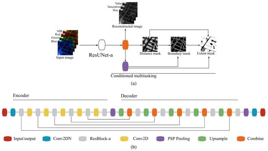
Figure 1.
Multi-task segmentation of ResUNet-a [13]. The emphasis of ResUNet-a lies with the multitasking approach. Producing the three segmentation masks is the main innovation of this network in boundary delineation. (a) ResUNet-a outline: Initially, a distance mask is derived from the feature map. This mask assists in determining a boundary mask. Together, these masks predict an extent mask. Additionally, a separate branch reconstructs the initial image. (b) Design of ResUNet-a.
The success of ResUNet-a has been demonstrated across various applications, proving its superiority over existing segmentation architectures. Its ability to efficiently capture contextual information, handle gradient issues, and perform multitasking for diverse output layers sets it apart as a valuable tool for semantic segmentation tasks.
2.2. Attention Gate and Attention U-Net
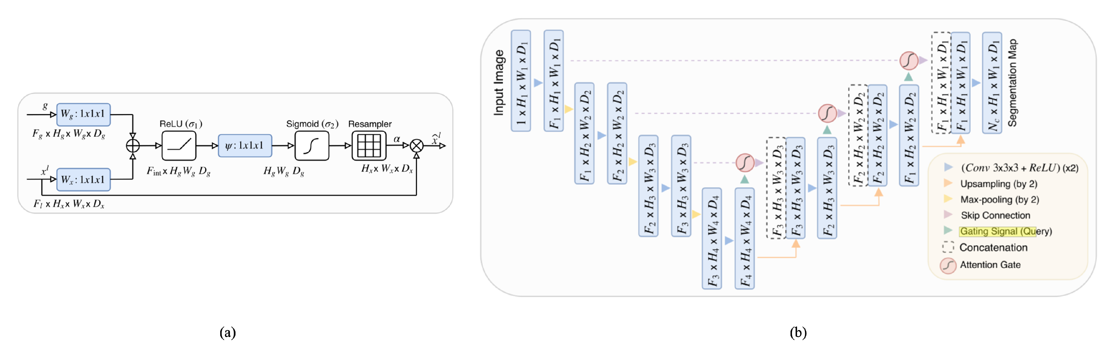
The concept of attention gating was jointly introduced in the collaborative works of Oktay et al. [25] and Schlemper et al. [26]. They showed that U-Net, when integrated with attention gates, enhances its proficiency in attending to the essential parts of an image, thus magnifying its precision in tasks like image segmentation. Figure 2 illustrates the attention gate and its implementation within the U-Net architecture. In the realm of neural networks, the concept of “attention” mirrors the human capability to concentrate on specific details within a vast array of information. The attention gate mechanism serves this exact purpose within the U-Net architecture which was proposed by Ronneberger et al. [21]. Within the U-Net’s architecture, skip connections, as discussed by Wang et al. [27], play an important role, transferring information from the network’s early layers directly to its later layers, ensuring the preservation of image details. However, the attention gate refines this process by allowing the network to accentuate the most important information from these skip connections. This refined information is identified through attention coefficients, values ranging between 0 and 1, which effectively spotlight significant image regions. This concept aligns with methodologies that value8 specific information channels, as seen in other works like sentence embedding in the work of Shen et al. [28]. The gating process, a key component of the attention gate mechanism, utilizes information from broader image scales to discern between vital and extraneous areas in these skip connections, as elaborated by Wang et al. [29]. This gating, similar to the attention mechanisms described by Mnih et al. [30], is strategically positioned before the merging of layers, filtering activations during the forward pass and ensuring learning focused on the pivotal regions during the backward pass.
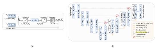
Figure 2.
Attention gate and attention U-Net [25]. (a) The attention gate flow chart. Two feature vectors enter, and they go through a series of operations to produce a feature map that is used to augment the input feature vector. (b) Attention U-Net, by placing the attention gate prior to the skip connections, learns how to pay attention to specific spatial features.
In the work of Tong et al. [31], their novel ASCU-Net architecture uses a triple-attention decoder block, which operates on the principles of the attention gate. Following the concatenation of feature maps derived from the encoder and up-sampling pathways, the attention gate comes into play. Its role is to apply a weighting mechanism that assigns varying degrees of importance to the features. These selectively weighted features subsequently undergo processing through spatial and channel-wise attention modules, resulting in an enhancement of spatial relationships and inter-channel correspondences, respectively. Other architectures, such as the one proposed by Nodirov et al. [32], adopted the attention gates in their original form. This application underscores the robustness of attention gates, as their model yielded noise-reduced features that significantly improved 3D segmentation. Deng et al. [33] took a slightly different path, integrating the attention gate within an encoder–decoder network, which subsequently led to the superior extraction of building boundaries. The innovative use of a high-pass filter as an attention mechanism was initially demonstrated by Susladkar et al. [34] in the domain of image dehazing. Their work emphasized the ability of a high-pass filter to prioritize high-frequency components within images, which are often associated with crucial details and edges. This unique approach allowed for a more effective dehazing process, as the filter helped to enhance critical information and suppress less important, lower-frequency components.
In the following section, we propose a parcel delineation method: a combination of a reduced version of the work presented by Diakogiannis et al. [12] with frequency domain attention. Unlike the original, our method employs only two masks. The incorporation of frequency domain attention ensures the extraction of a more refined edge mask, thereby enhancing the delineation performance of our approach.
3. Methodology
In this section, we introduce a modified version of the U-Net architecture tailored specifically for parcel boundary delineation in satellite imagery. Our modifications aim to address the unique challenges of this task and improve accuracy and precision. We explain the utilization of two types of masks, namely edge masks and extent masks, within the architecture. Additionally, we outline the structure of the network, which is composed of an encoder path and two decoder paths.
3.1. Base Network Architecture
The common practice when it comes to multitasking segmentation for boundary delineation is the use of three separate masks, as was proposed in Diakogiannis et al. [13]. However, in our approach, we choose to utilize only two output masks, each with its distinct role, simplifying the process while ensuring functionality. The primary mask acts as the conventional extent mask, giving a visual representation and laying out the boundaries of individual parcel regions in the imagery. This mask is key to understanding the basic layout of the features being observed.
The second mask, which we refer to as the edge mask, plays a crucial role in this architecture. It specifically targets and depicts the shared boundaries or edges between the adjoining segmentation masks. The reasoning behind the incorporation of this edge mask is based on the semantic segmentation of Bertasius et al. [35] and Marmanis et al. [36]. These studies have shown the significant impact that a more accurate boundary delineation can have on the overall performance of the segmentation task. Consequently, by adopting this approach, we aimed to explore the potential of these insights, improving the accuracy of our boundary delineation.
Furthermore, our approach diverged from that of Diakogiannis et al. [12] by focusing only on the utilization of U-Net as our primary network structure. We refrained from integrating additional layers of complexity, which, while potentially adding to the functionality, could also make the system more susceptible to overfitting and increase computational demand.
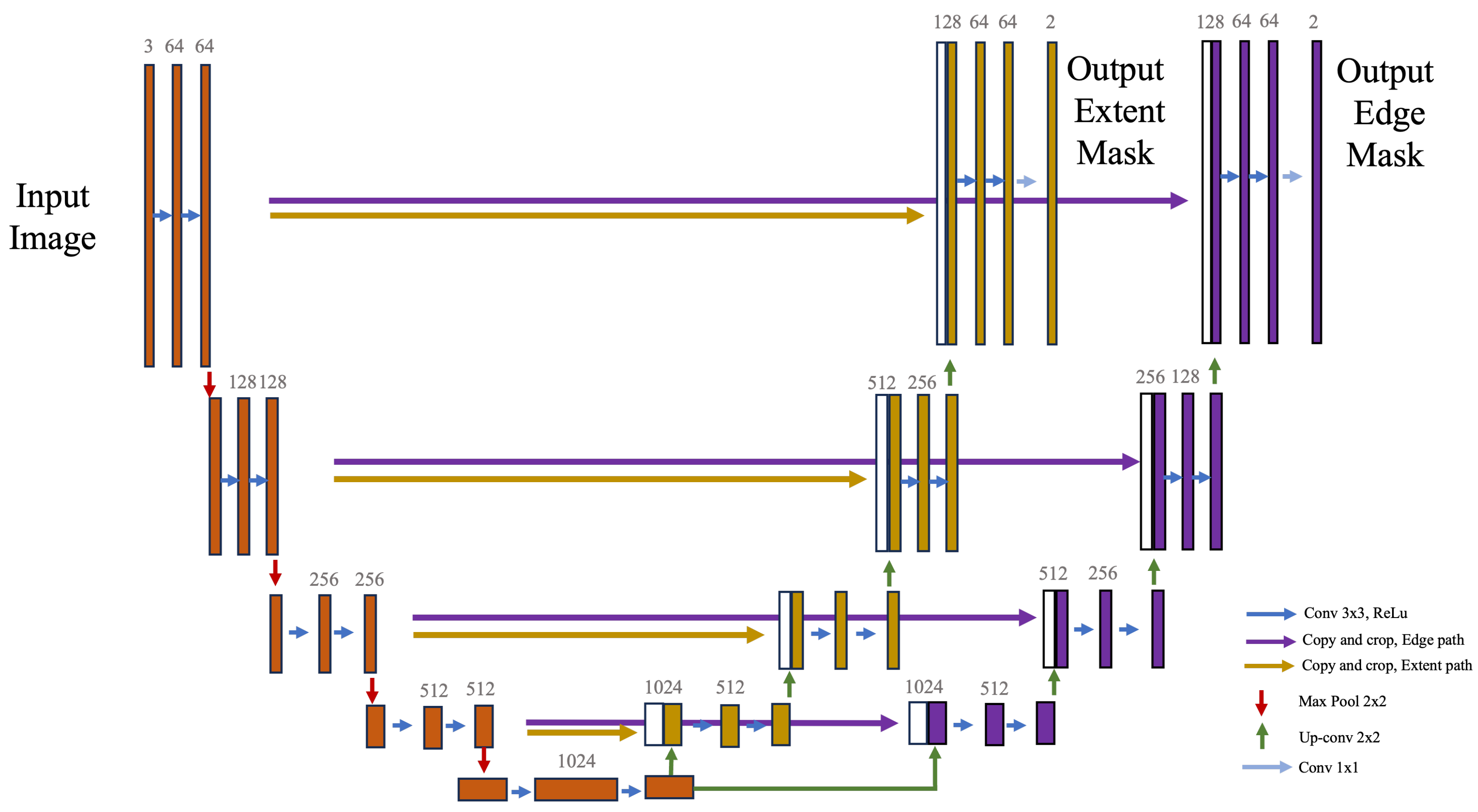
For this purpose, we used the U-Net architecture proposed by Ronneberger et al. [21]. We modified the U-Net architecture to have one encoder path and two decoder paths. The decoders are independent from each other and do not share any connections. This allows for independence of the connections between the encoder and each of the two decoders. This architectural decision allows each decoder to independently learn and refine the information extracted from the encoder’s features. This independent learning capability of the decoders provides an important advantage: it enables the system to capture and incorporate essential boundary-related features during the decoding process more effectively. In essence, it allows for a higher degree of flexibility in managing and interpreting the information. This results in a more accurate representation of the boundaries, demonstrating the value of our approach for segmentation tasks. The two-headed U-Net base architecture can be seen in Figure 3.
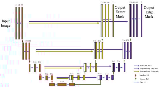
Figure 3.
A schematic of the modified dual-headed U-Net architecture implemented in our study. In contrast to the original U-Net architecture that features a single expanding path, our design requires two expanding paths: the edge path and the extent path. These are trained concurrently, demanding the encoder to adapt and guarantee precise outputs from both paths. Despite the modification, this design maintains the contracting path identical to the original U-Net model.
3.2. Frequency Attention Gate
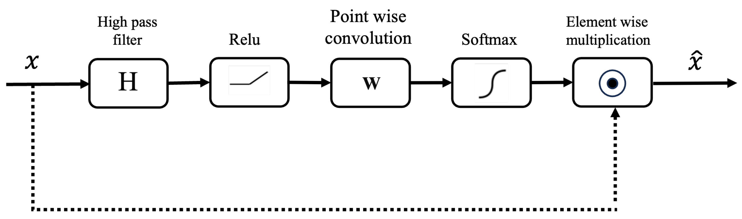
In our proposed methodology, we introduce a novel approach to the attention mechanisms by placing emphasis not just on the spatial locations within an image but also on its frequency-specific features. Edges correspond to high-frequency components in an image, as explained in the work of Papasaika [37]. Our innovation stems from the fact that the quality of boundary delineation is determined by the edge mask. To refine this mask, we have re-engineered the traditional attention gate. Before processing the raw feature vector directly, it is first subjected to a high-pass filter. This step accentuates the high-frequency components of the image, which are synonymous with edges and fine details. By preconditioning the attention coefficients to favor these high-frequency components during the learning phase, the network becomes more adept at identifying and amplifying edges. Such a shift in focus is crucial, as it can significantly enhance the outcomes of the edge detection task. A depiction of this modified attention gate is provided in Figure 4. The high-frequency attention gate can be explained as follows.
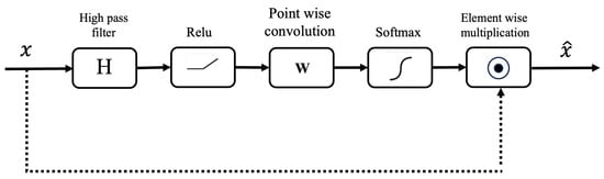
Figure 4.
Proposed high-frequency attention gate. The figure illustrates the attention gate module, which enhances feature representation in neural networks by incorporating spatially adaptive attention weights. It shows the flow of operations, including high-pass filtering, ReLU activation, convolutional operations for attention weight computation, softmax normalization, element-wise multiplication, and feature fusion. The attention gate selectively highlights important regions while suppressing less relevant areas, improving the model’s ability to capture fine-grained details.
High-pass filters accentuate the high-frequency components and diminish the low-frequency components. This operation is mathematically exemplified by the convolution operation:
where:
- X represents the input feature vector.
- H signifies the high-pass filter.
- ∗ denotes the convolution operation.
- is the resultant high-pass filtered feature vector.
The high-pass filter H for 2D data is detailed as:
When applied, the filter emphasizes rapid intensity changes in the feature vector, representing transitions such as edges or fine details. For a feature vector with a horizontal transition, for instance, the filter will yield a positive response at the onset of the transition and a negative one at its end, thus highlighting the presence of such transitions.
The ReLU (Rectified Linear Unit) function is then utilized on the high-pass filtered feature vector:
By introducing non-linearity into the model through the ReLU function, the network becomes adept at learning and adjusting from the error.
Subsequently, an attention map is derived using a convolution operation with learnable weights:
where W symbolizes the learnable weights. This attention mechanism enables the model to concentrate on specific parts of the feature vector, assigning more importance to critical features.
For normalization, a softmax activation is employed on the attention map:
This ensures the attention map values to lie between 0 and 1, thus highlighting certain features more than others.
The attention map is integrated with the original feature vector through element-wise multiplication to produce the attended feature vector :
where ⊙ represents element-wise multiplication.
Redesigning the attention this way ensures that the emphasized features are the high-frequency features, essentially conducting attention in the high-frequency band of the image. These features are of extreme importance to our problem, and any improvement made in detecting edges reflects directly on the quality of the final parcel delineation results.
3.3. Final Network Architecture
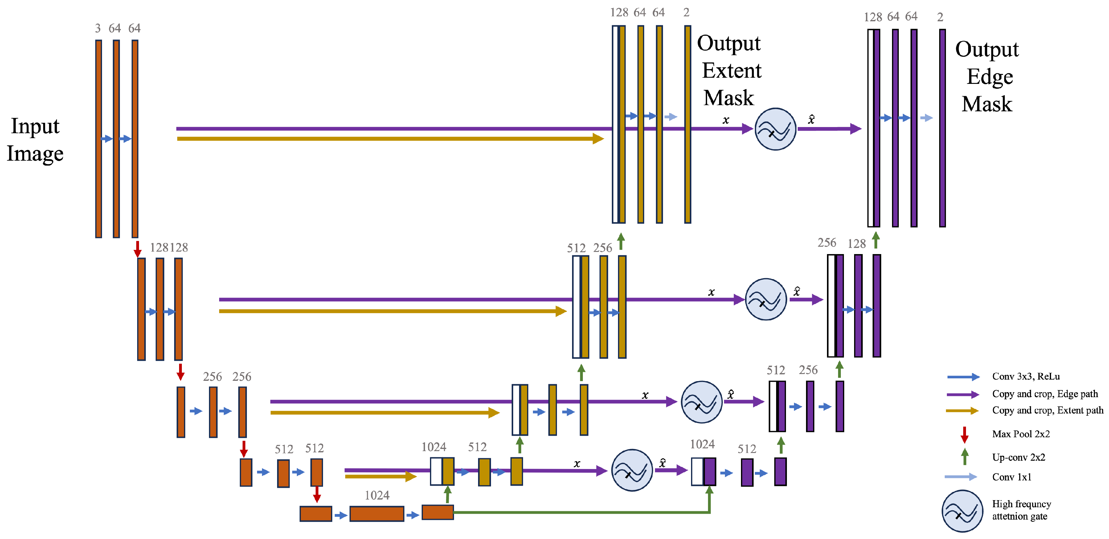
The final network architecture seen in Figure 5 incorporates attention gates, following the methodology proposed by Oktay et al. [25]. These attention gates are strategically placed prior to the concatenation of cropped features and upscaled features, in the expanding path responsible for the edge mask. This allows for the effective integration of attention-based feature vectors within the U-Net framework. The resulting feature vector from the attention mechanism is then combined with the upscaled feature vector, a common practice in U-Net architectures.
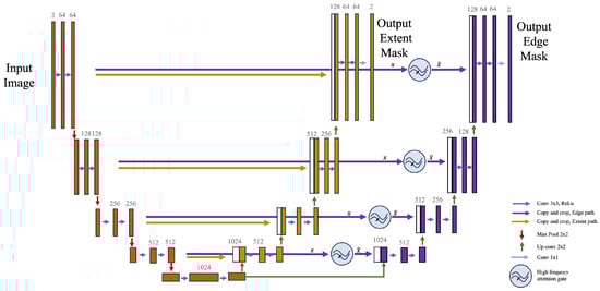
Figure 5.
Final network architecture after adding the high-frequency attention gates.
At its foundation, the network is designed with a singular encoder of depth 5 and two parallel decoders. The encoder initiates with an input layer, followed by four downscaling stages, resulting in a total of five layers. Each layer in the encoder is characterized by two sequences of 3 × 3 convolutions, complemented by batch normalization and ReLU activation functions. The number of filters in these layers commences at 64, doubling consecutively through configurations of 64, 128, 256, 512, and ultimately 1024 filters.
Transitioning from the encoder, the network diverges into its two decoders. Each decoder embarks on a series of upscaling steps, reducing the depth from the foundational 1024 filters progressively through 512, 256, 128, and culminating at 64 filters. Depending on the specific model configuration, these upscaling operations can adopt either bilinear upsampling or transpose convolutions.
The distinguishing feature of FAUNet is the integration of frequency attention mechanisms. The attention gates are embedded within the framework, situated after the upscaling layers of the decoders. These gates employ high-pass filters to formulate attention maps, empowering the network with the capability to accentuate specific features selectively. Each decoder delivers an output map that corresponds to the pre-defined class depth of 2, one corresponding to the extent mask and the other to the edge mask.
3.4. Loss Function
In the proposed approach, the loss function incorporates both Dice loss and cross-entropy loss, as discussed by Sudre et al. [38]. These are applied separately on the main regions of interest and the edge areas in an image segmentation task. This harmonized loss function serves to optimize the model for global and local features in the segmentation task, which can lead to more precise and robust results.
The Dice loss, derived from the Sørensen–Dice coefficient, is an established metric for the assessment of image segmentation models. This coefficient, as described by Milletari et al. [39], measures the similarity between two binary samples and can vary between 0 and 1. A Dice loss that is closer to zero signifies a greater overlap between the predicted and actual masks, indicating a better segmentation performance. In the case of both main and edge areas, the Dice loss is calculated after applying a softmax function to the predicted probabilities output by the model, effectively normalizing these probabilities within the range of 0 to 1. The actual masks are one-hot encoded to match the dimensionality and format of the predictions, providing a suitable basis for comparison.
Cross-entropy loss is a prevalent loss function for classification tasks. It measures the dissimilarity between the predicted probability distribution and the true distribution. The combined cross-entropy loss is calculated separately for the edge predictions and the mask predictions, with the results combined to encourage accurate classifications at the pixel level.
The total loss function is designed as the average of the edge Dice loss, the extent mask Dice loss, and the combined cross-entropy loss. This weighted combination of different losses allows for balancing between pixel-wise accuracy, emphasized by the cross-entropy loss, and the overlap of the predicted and true segmentation areas, which is captured by the Dice loss. As highlighted by Yeung et al. [40], the specific combination of these losses is a design choice, influenced by the nature of the data, the segmentation task, and the desired characteristics of the model’s performance.
The given loss function can be mathematically represented as follows:
Given , as the true and predicted extent masks respectively, and , as the true and predicted edge masks respectively, the total loss function is represented as:
Here, is the Dice loss, defined as:
and is the cross-entropy loss, defined as:
In these equations, A and B are the true and predicted labels, respectively, n represents the total number of elements, and is a small constant to ensure numerical stability. The sums are over all elements in the masks or edges.
The Dice loss is calculated for both the edge masks and extent masks, while the cross-entropy loss is also calculated for both the edge masks and extent masks. The final loss is a weighted average of these four components, balancing the contributions of pixel-wise accuracy from the cross-entropy loss and overlap accuracy from the Dice loss.
3.5. Post-Processing
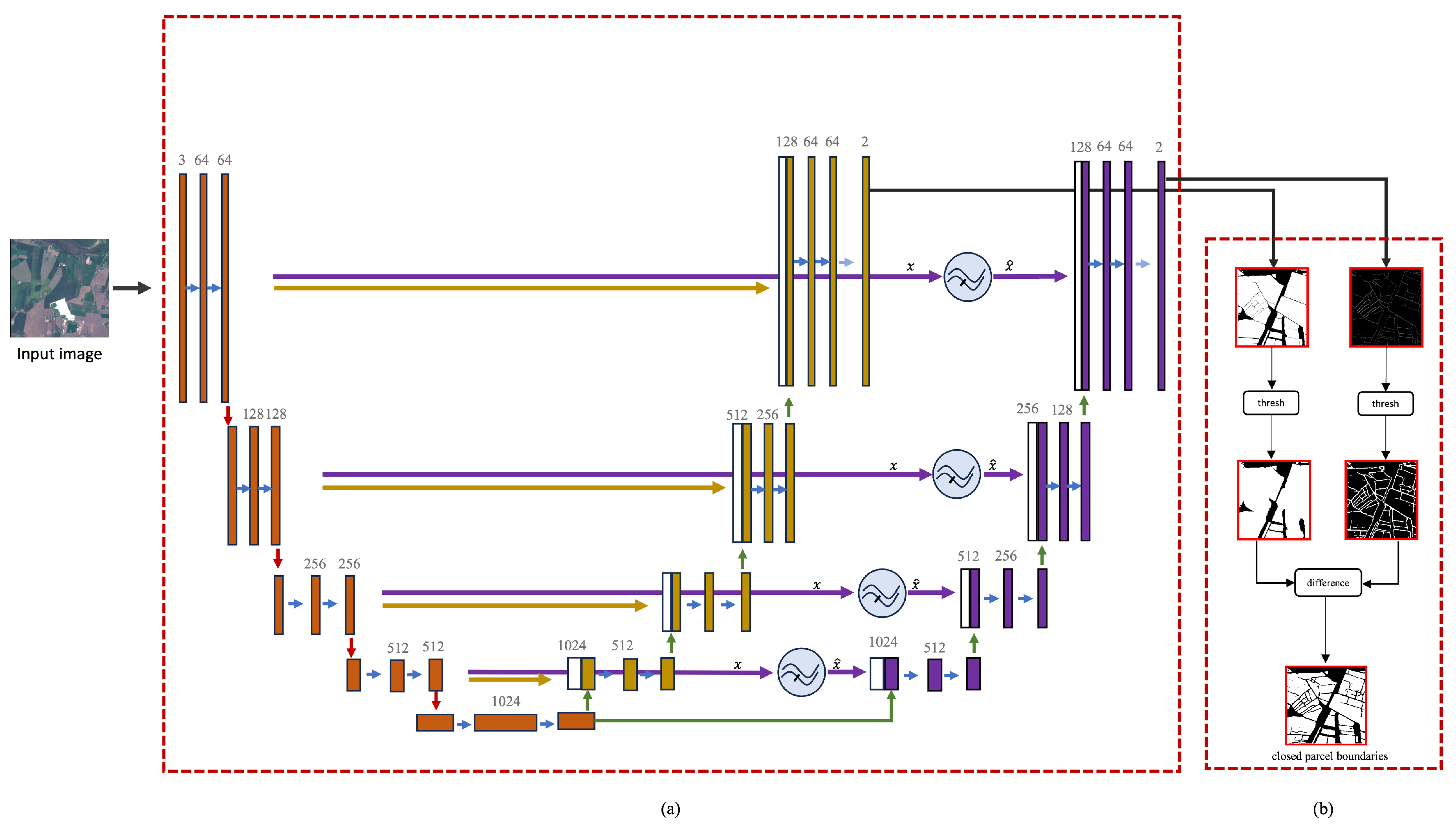
After obtaining the edge and extent masks from the dual expanding paths of our network, we need to combine them to create complete parcel boundaries. To achieve this, we use a modified version of the cutoff methodology described in [13]. To maintain simplicity of post-processing, we opted not to perform threshold optimization, instead using a fixed threshold value. This approach simplifies the parcel boundary generation process. Employing a constant threshold also emphasizes the need for precise and accurate segmentation results. The post-processing pipeline and the entire model pipeline can be seen in Figure 6b.
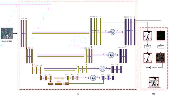
Figure 6.
The complete pipeline including the model and the post-processing step. (a) FAUNet, (b) cut-off post-processing method.
3.6. Accuracy Assessment and Error Metrics
To ensure reliable and comprehensive evaluation of boundary delineation algorithms, it has become a common practice to adopt established metrics that have gained popularity in this domain [13,18]. These metrics encompass a combination of pixel-based error measurements, including precision, recall, F1 score, intersection over union (IoU), and overall accuracy (OA), which offer detailed insights into the algorithm’s performance at the pixel level. Moreover, to address broader structural aspects, we also incorporate object-based metrics, namely over-segmentation (OS) and under-segmentation (US) [41] and . The pixel-based evaluation metrics are mathematically defined as:
Object based metrics, over-segmentation OS, and under-segmentation US are as follows: Assume is the ground-truth parcel that has the largest area of intersection with the predicted parcel , , where m is the number of predicted parcels. Let and be the areas of and , respectively, and be their overlapping area. We obtained an over-segmentation error, , and an under-segmentation error, :
where
- TP refers to the number of true positives at the object level. In the context of object detection, a true positive (TP) is defined as a detected object that has an intersection over union (IoU) overlap of more than 50% with a ground-truth object.
- FP refers to the number of false positives at the object level.
- FN refers to the number of false negatives at the object level.
According to [41], when the over-segmentation (OS) metric approaches zero, it signifies lower over-segmentation errors, and when the under-segmentation (US) metric approaches zero, it indicates lower under-segmentation errors.
3.7. Dataset
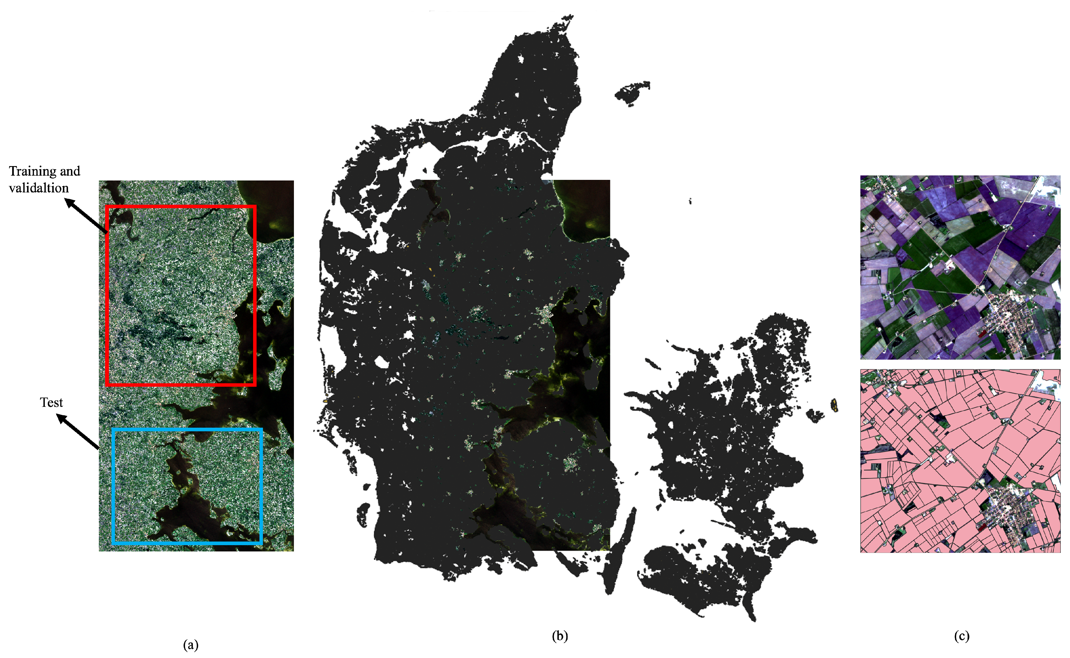
The Denmark dataset consists of two parts: the parcel boundaries, which are sourced from the European Union’s Land Parcel Identification System (LPIS), and the mosaic, which was sourced through the Google Earth Engine as described by Rieke [42]. The mosaic integrates two unobscured top-of-atmosphere (TOA) Sentinel-2 images dated 8 May 2016. These images present a true-color composite with a spatial resolution of 10 m per pixel. Captured during the early growth period, they comprehensively span the eastern expanse of Denmark, covering an impressive 10,982 × 20,978 pixels and encapsulating an area of approximately 20,900 km2. This dataset, as described by Rieke [42], contains the diverse landscape of agricultural parcels in Denmark, each distinct in size and morphology. The vector data can be sourced from (https://collections.eurodatacube.com/, accessed on 1 July 2023). The geographical focus of this study is centered on central Denmark, as visualized in Figure 7. Defined by the Sentinel-2 satellite image mosaic seen in Figure 7a and the corresponding digitized agricultural parcels, overlaid over the raster in Figure 7b, this region spans the eastern part of Denmark, extending into the Baltic Sea and reaching the island of Funen, Denmark’s second-largest island. Dominated by agricultural activities, the area is characterized by its temperate climate and predominantly flat terrain. A closer visualization of the raster data and the overlaid vector can be seen in Figure 7c. For a detailed analysis, we adopted a methodical geographical division of the dataset. The top half is allocated for training and validation, while the bottom half serves as the domain for testing unseen data. Such a geographical division within a single dataset is consistent with established practices in boundary delineation research. For instance, as highlighted by Waldner and Diakogiannis [13], ResuNet-a utilized varied tiles spanning their entire study area for training and testing. Similarly, the data split used in SEANet is identical to the split we used [20]. This division strategy was not just in adherence to existing practices but was also chosen to negate potential complications introduced by spatial autocorrelation, as discussed by Karasiak et al. [43]. After this segregation, 80% of the northern part of the data is channeled into training, with the remaining 20% earmarked for validation. This division was performed on a chip basis with random selection. For pre-processing, normalization was employed to unify the distribution of the pixel values of the images. By scaling the pixel values to the range [0, 1], normalization ensures consistency and facilitates better convergence during training. To augment the number of samples, an overlap of 128 pixels was systematically introduced. To ensure the quality of the data, we excluded empty parcels or those where the parcel footprint was less than 20% of the image. Such careful exclusions played a crucial role in mitigating potential skew from negative samples, as noted by Li et al. [20]. The algorithm facilitating this division owes its origins to the methodology presented by Rieke [42]. A comprehensive visualization of our dataset and its methodical divisions is shown in Figure 7.

Figure 7.
Denmark dataset. (a) The mosaic spanning the central east of Denmark. The red rectangle represents the region used for training and validation while the blue rectangle represents the area used for testing. (b) The vector of the annotated fields covering Denmark. (c) A zoomed-in sample of the dataset; the upper part is the raster, while the lower image is the annotated parcel boundaries.
4. Results
4.1. Module Comparison
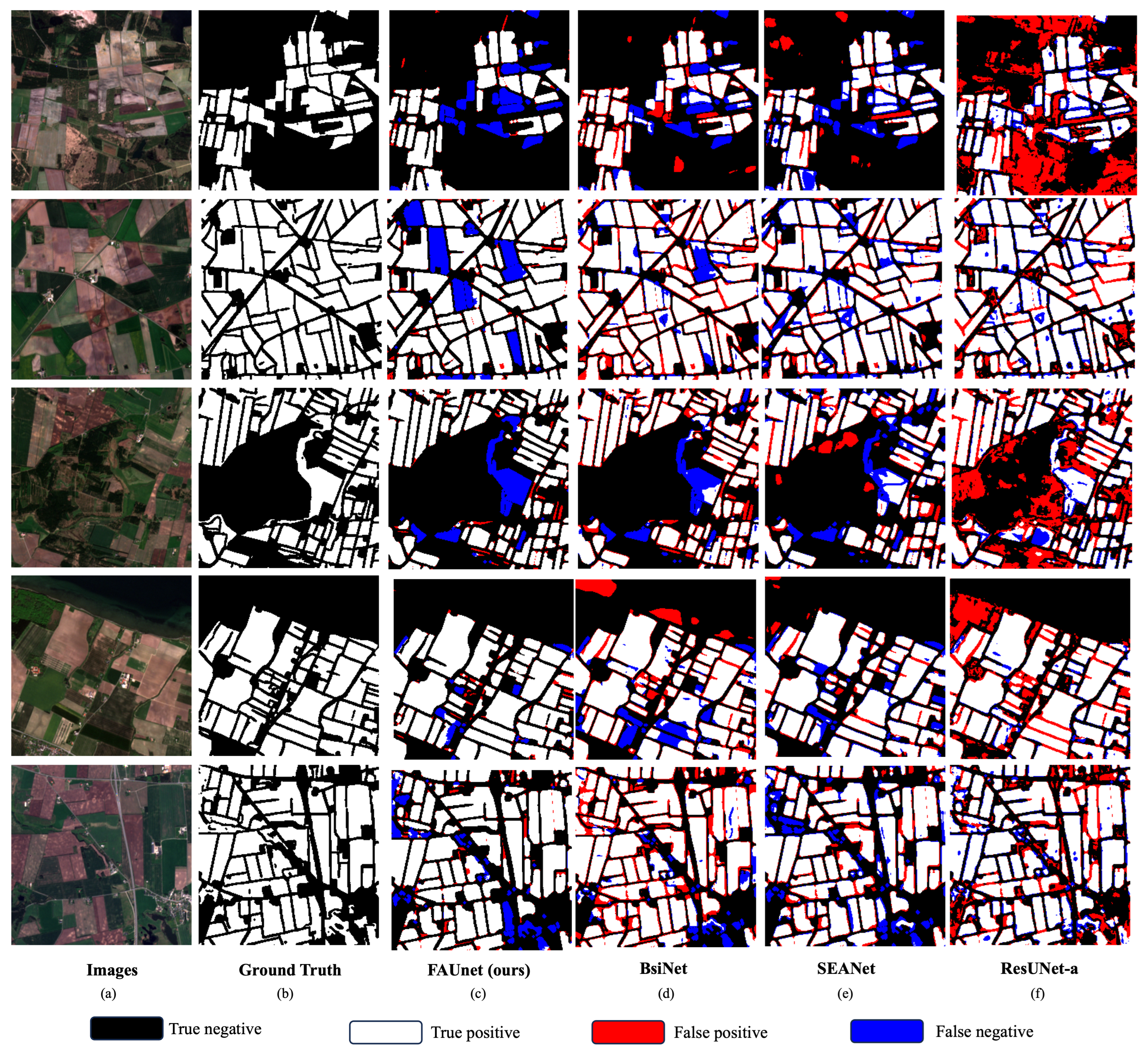
Figure 8 acts as a visual example that showcases a comparison of performance between FAUNet, ResUNet-a, BsiNet, and SEANet. After careful examination, it becomes clear that the results from FAUNet show the highest performance compared to the ground truth. This holds true for both the number of parcels identified and their overall visual features, surpassing the achievements of the other models. An important point to highlight is FAUNet’s capability to accurately define parcel boundaries. This is an area where it clearly surpasses its counterparts. FAUNet’s results contain a significantly lower number of false positives, indicated by the lack of red pixels in its result. However, FAUNet falls short when it comes to detecting some parcels, which is clearly showcased by the presence of regions of blue pixels. It is important to note that the frequency attention gate aids in improving the edge mask, thus enhancing the detected boundaries, but it does not affect the extent mask, which may lead to entire parcels being undetected. This is exemplified by the visual representation seen in the Figure 8. Moreover, visually, ResUNet-a and BsiNet have a higher rate of mis-detections that SEANet and FAUNet. This is clear by the larger presence of red pixels. BsiNet, however, performs better than ReUNet-a.
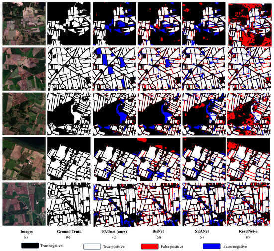
Figure 8.
Results comparison. (a) Input image. (b) Ground truth. Parcel delineation results obtained by (c) proposed FAUNet,(d) BsiNet, (e) SEANet, (f) ResUNet-a.
Furthermore, the visual analysis highlights FAUNet’s efficacy in mitigating under-segmentation errors in comparison to the other models. This advantage can be attributed to the more distinct and well-defined edge mask of FAUNet, which contributes to its more accurate parcel boundary delineation. Conversely, ResUNet-a shows acceptable performance in terms of over-segmentation error. However, it is important to note that this advantage can be attributed to a tendency toward under-segmentation. This issue highlights the trade-off between ResUNet-a’s higher detection rates and its overall reduced accuracy compared to the other models. BsiNet and SEANet both have similar performance when it comes to correctly combining or splitting parcels, with SEANet having a slight edge over BsiNet.
In summary, Figure 8 visually demonstrates how FAUNet outperforms other models in precision but falls short in recall. FAUNet provides clear parcel boundary delineation and effectively reduces false positives while keeping the number of false negatives low. Moreover, it maintains a good balance between over-segmentation and under-segmentation, collectively positioning it as an improvement over the other models.
Table 1 and Table 2 show a clearer difference between the models. FAUNet outperforms the other models in both pixel-based metrics and object-based metrics.

Table 1.
Pixel-based metrics.
Table 2.
Object-based metrics.
Table 1 presents a detailed performance comparison of five different segmentation models: U-Net, ResUNet-a, BsiNet, SEANet, and FAUNet. These models are evaluated based on pixel-based metrics, including precision, recall, overall accuracy (OA), F1 score, and intersection over union (IoU). Starting with the U-Net model, it has a decent recall score of 0.8256, but it falls short in other metrics compared to the other models. In particular, its IoU and F1 scores are the lowest among the models, highlighting areas for potential improvement. ResUNet-a outperforms the other models in terms of overall accuracy, achieving a score of 0.9174. Its precision and recall scores are also commendable, and its IoU and F1 scores show improvements over those of the U-Net model. One the other hand, BsiNet provides competitive results with its recall score of 0.8557 and an overall accuracy of 0.8932, but it struggles with precision, achieving a score of 0.8358. SEANet demonstrates a balanced performance, with the highest recall score of 0.8713 among the models and a good overall accuracy. Its F1 score and IoU are improvements over both U-Net and ResUNet-a, suggesting that SEANet is a more balanced model for pixel-based segmentation, but it still does not perform well in precision, scoring a modest 0.8458. Finally, FAUNet comes first in precision, F1 score, and IoU, scoring 0.9047, 0.8692, and 0.7739, respectively. Its recall score and overall accuracy, while not the highest, are quite competitive, adding to its credentials as a robust parcel boundary delineation model. To summarize, while each model has its strengths and areas for improvement, FAUNet emerges as the leading model for pixel-based segmentation tasks based on these chosen metrics, with the highest precision score, F1 score, and IoU.
In Table 2, a comprehensive evaluation of segmentation methodologies is showcased, focusing on the comparative effectiveness of five state-of-the-art architectures: U-Net, ResUNet-a, BsiNet, SEANet, and FAUNet. The benchmarking relies on three metrics, providing a multi-faceted perspective on their performance capabilities: over-segmentation (OS), under-segmentation (US), and the F1 score at the object level (). Diving into the specifics, FAUNet outperforms the other models when it comes to parcel boundary delineation. We can make this assertion based on its performance in minimizing the OS and US errors, with respective values of 0.0341 and 0.1390. The lower these values are, the closer the predicted segmentations are to the ground truth, making FAUNet’s superiority evident. Moreover, FAUNet’s better performance is exemplified with an score of 0.7734, the highest among the other models. This high score emphasizes its effectiveness at harmonizing precision and recall. BsiNet achieves an OS value of 0.0476 and a US value of 0.2993. In the context of parcel boundary delineation object-based metrics, these results indicate that BsiNet effectively balances its segmentation tasks. A lower OS value suggests that BsiNet is less likely to erroneously include extra areas in its segmentation. At the same time, its US value shows that it also minimizes the chance of missing genuine parts of objects. Thus, the model demonstrates a notable balance of precision in marking object boundaries without overly missing or adding segments. This balance is vital for ensuring accurate and reliable segmentation outcomes. SEANet, on the other hand, delivers a noteworthy performance. While not establishing the best metric in any single category, its commendable score of 0.6705 indicates its reliable efficacy. This benchmark positions SEANet as a consistently performing architecture, especially when taking into account its great US metric, obtaining a low 0.0698 US error while maintaining a reasonable 0.2429 in the OS metric. This means that even if SEANet combines the detected parcels, it does not split them in other cases and it detects a high number of them. On the other hand, both U-Net and ResUNet-a have higher OS and US values. Such elevated figures indicate an inclination towards segmentation inaccuracies, splitting some parcels while combining others. U-Net registers OS and US values of 0.1888 and 0.2436 respectively, while ResUNet-a performs a bit better with 0.1434 and 0.2123. Further, their scores are 0.4827 for U-Net and 0.5043 for ResUNet-a.
4.2. Training Process and Computational Load of Different Models
All models were trained using codes and hyperparameters optimized by their respective authors. Each model underwent 100 epochs of training to ensure consistency in the evaluation. The same training and validation data were used for all models.
For training FAUNet, a random search was employed to select optimal learning rates and weight decay parameters. Ultimately, the default values of a learning rate of and a weight decay of proved to be ideal. A fixed batch size of 12 was used across all models due to hardware limitations.
Training was conducted on an Nvidia RTX 4070 graphics card. The number of parameters and floating-point operations per second (FLOPs) were calculated for each model and are presented in Table 3. Notably, despite the inclusion of attention weights and high-pass filter weights, FAUNet exhibited only a modest increase in both parameters and FLOPs compared to the standard U-Net with two heads. BsiNet emerged as the lightest and fastest model, outperforming FAUNet in computational efficiency, while SEANet and ResUNet-a demonstrated higher computational complexity.
Table 3.
Estimates of FLOPs (floating-point operations per second) and Parameters for different models.
4.3. FAUNet Test Region Results
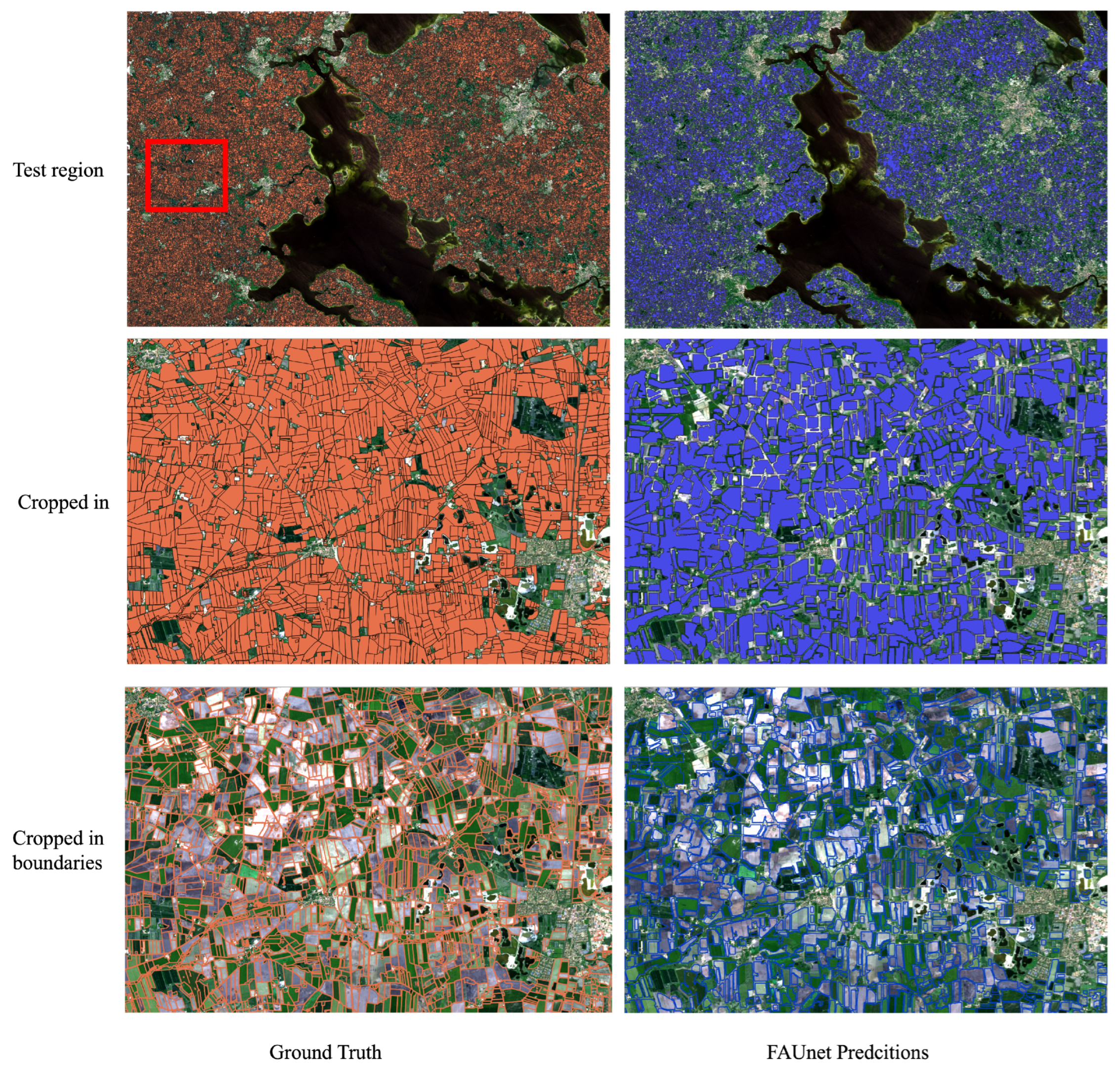
Conducting inference on the entire test region presents a set of intricate challenges. The test region encompasses more than 70 million pixels, with dimensions of 10,000 pixels in width and 7000 pixels in height. To ensure a seamless inference process devoid of sliding window artifacts, we perform three separate inferences using a 256 × 256 sliding window, each starting at different points: 0, 85, and 175. This effectively simulates conducting a single inference with a step size of 85 pixels, preserving the integrity of the results. Moreover, we leverage test–time augmentation techniques, including horizontal flips, vertical flips, and their combinations, resulting in a total of 12 separate inferences. Each of these inferences comprises 1107 256 × 256 image chips and consumes approximately 18.7 s. Subsequently, the results from these individual inferences are consolidated to obtain the final outcome. However, it is important to note that this final result is initially in raster form. To convert it into vector form, we employ morphological operations such as erosion, dilation, and closing to refine and separate field instances. Following this, we extract the boundaries of each object. Finally, we transform the resulting parcel data into vector format, accurately positioning them within the geographical coordinates of the initial dataset. The results obtained from FAUNet in the form of vector shapefiles are depicted in Figure 9. These shapefiles are registered to the precise geographical location of the original dataset. For a closer examination of the resulting boundaries, refer to the second and third rows of Figure 9.
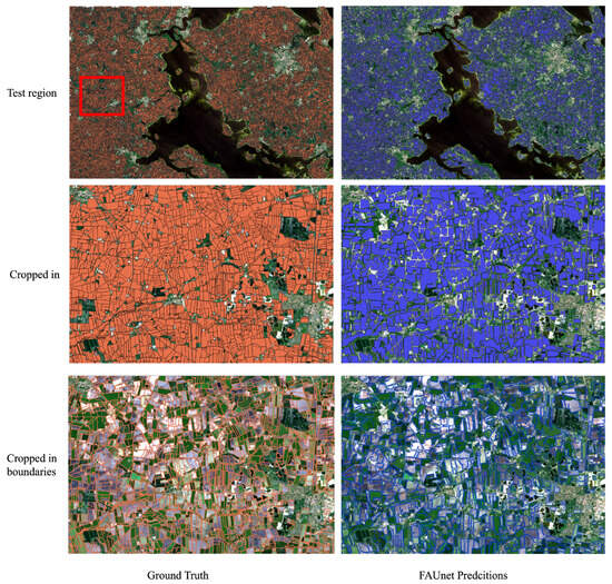
Figure 9.
FAUNet inference conducted on the entirety of the test region. The left column displays the ground-truth vector data, while the right column showcases the resulting vector data generated by FAUNet. A closer look at the test region can be seen in the second and third rows of the figure. The cropped in region is labeled by a red box in the first row.
4.4. Temporal Transferability Analysis
Upon evaluating our model, which was originally trained on 2016 satellite images on a 2023 data subset, intriguing findings were observed. Despite the seven-year gap and potential variances between the historical ground truth and current data, the model displayed commendable resilience with almost no degradation in pixel-based error metrics, as seen in Table 4. This suggests a high degree of consistency and adaptability at the micro-level. However, when examining object-based metrics seen in Table 5, there was a noticeable dip in performance. While this decline is present, it is crucial to note that the model still delivers results within an acceptable range, especially considering the significant time difference. This dual insight provides valuable information about the model’s strengths and potential areas for further refinement to ensure holistic temporal robustness.
Table 4.
Time Transferability Metrics Table—Pixel Based.
Table 5.
Time transferability metrics table—object based.
Figure 10 provides a visual representation of FAUNet’s performance on 2023 imagery. A closer observation reveals that the ground truth and the resultant images do not align precisely for each field, likely contributing to the decline in object-based metrics. Despite this, FAUNet successfully delineates parcels, with only a slight uptick in missed pixels. While there is a tendency for the model to under-segment parcels, its overall performance remains commendable given the temporal challenges it faces.
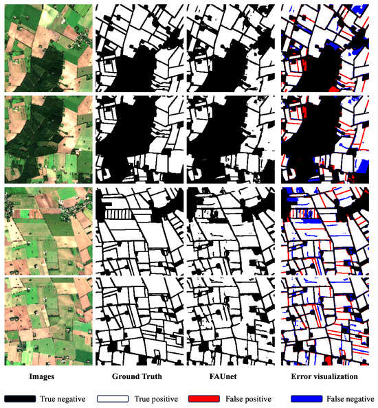
Figure 10.
FAUNet results on for imagery obtained in September 2023.
4.5. Ablation Study
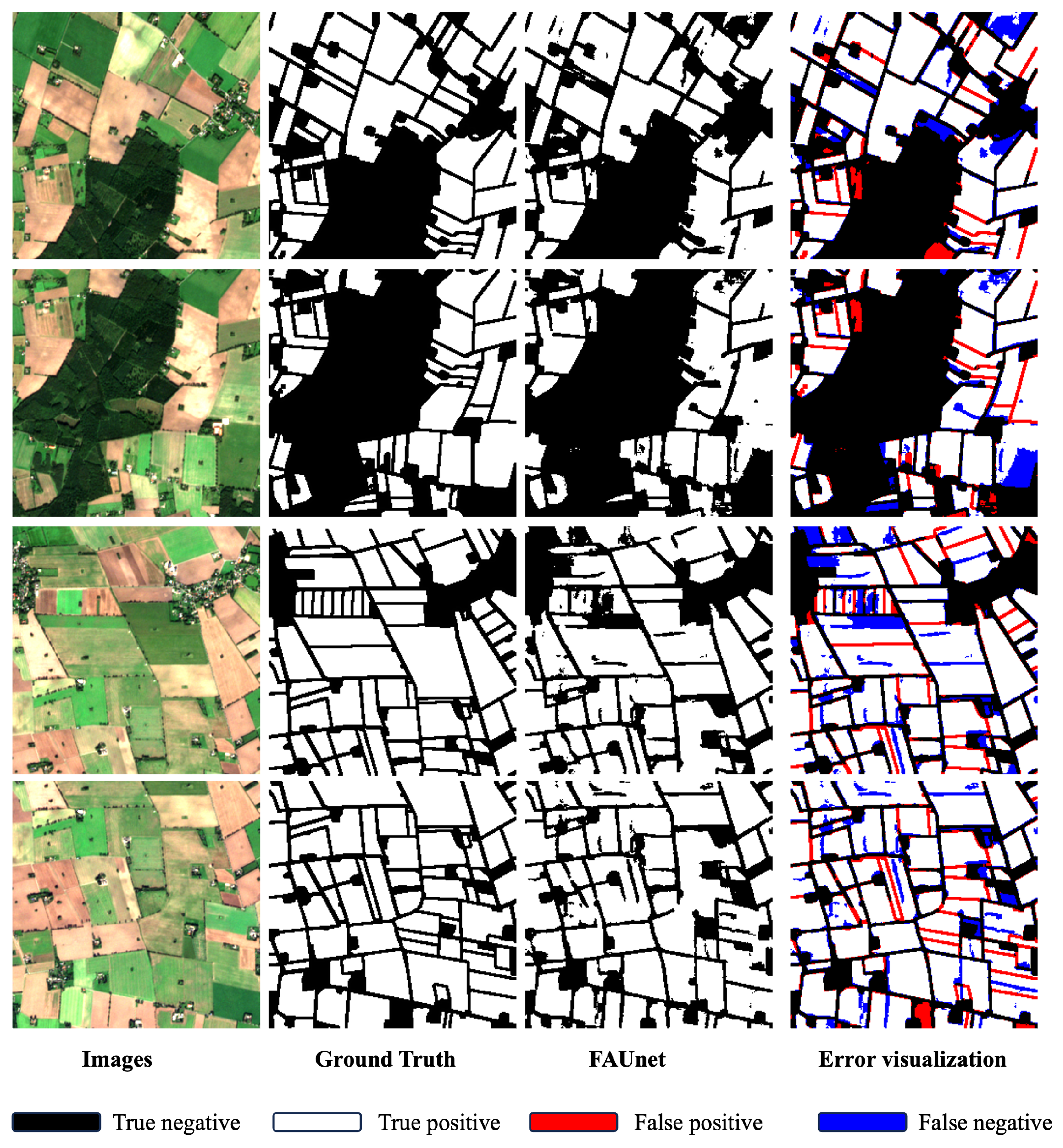
Our study investigates how the frequency attention model impacts the architecture of our neural network. We conducted experiments comparing the quality of edge masks between the standard U-Net model and our previously introduced FAUNet, which incorporates the frequency attention mechanism.
The results, presented in Figure 11, illustrate the relative performance of FAUNet when compared to the conventional U-Net. Our evaluation primarily focuses on the accuracy of the edge mask and the overall output.

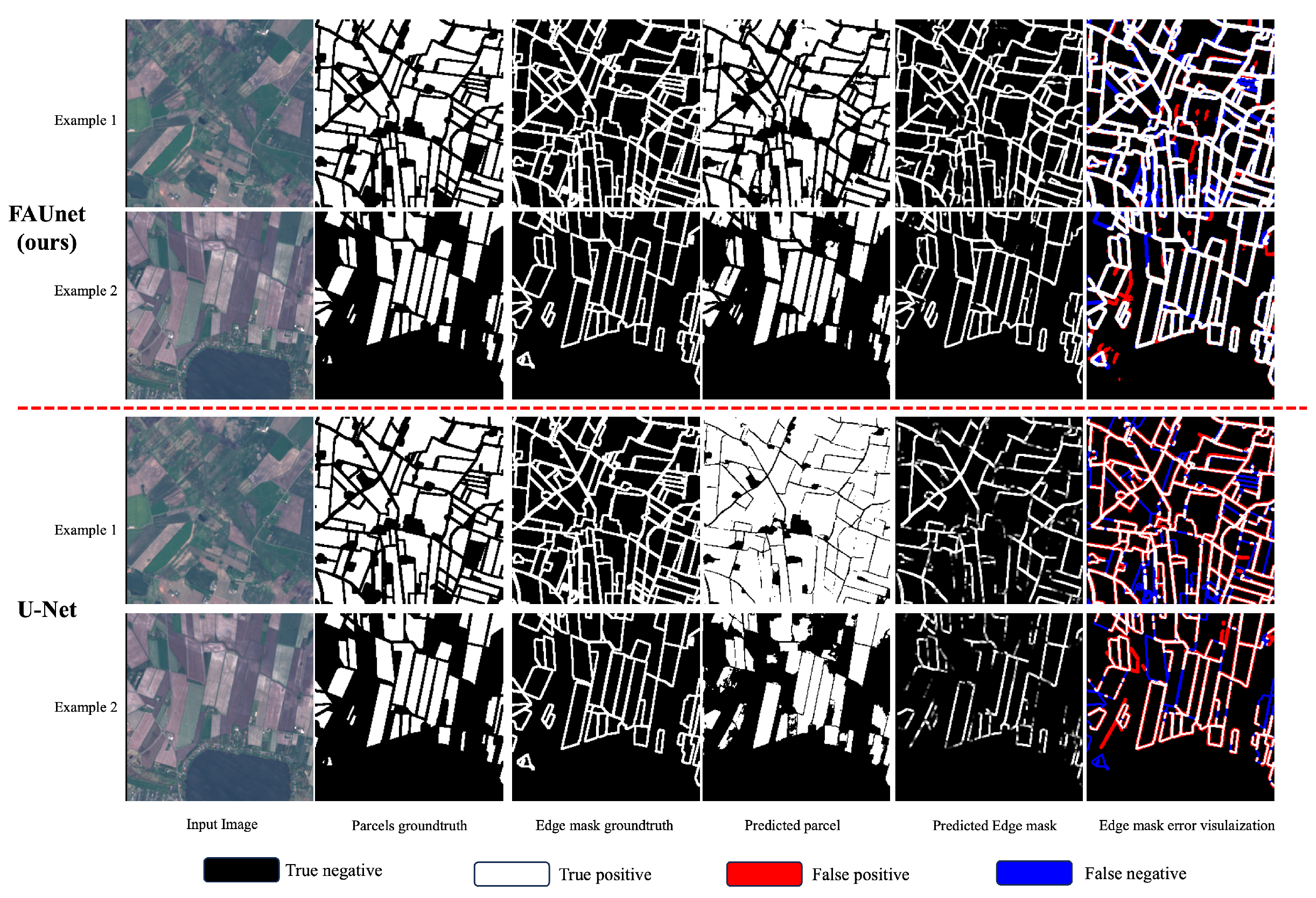
Figure 11.
Comparison of results and edge masks between FAUNet and U-Net. Example 1 and Example 2 serve as input for both U-Net and FAUNet. The first two rows depict the results of FAUNet, while the third and fourth rows depict the results of U-Net.
Figure 11 provides a comprehensive view of the outcomes for both FAUNet and the conventional U-Net model. It includes input images, ground-truth parcels, and ground-truth edge masks. The final column visually represents error metrics, showing true positives, false negatives, and false positives, with a specific focus on boundary pixels. To enhance clarity, we have implemented a color-coded scheme. White pixels indicate agreement between the output edge mask and the ground truth, while red pixels represent edge pixels that are present in the ground truth but missing in the model’s prediction. Conversely, blue pixels represent pixels present in the model’s output but not in the ground truth. This color scheme effectively illustrates the substantial impact of the frequency attention mechanism on performance. Figure 11 demonstrates the improvements in FAUNet’s performance compared to the conventional U-Net. In the error visualization of FAUNet, white pixels predominate, signifying a significant presence of true positives, with fewer occurrences of blue and red pixels. Conversely, the U-Net visualization has fewer white pixels and more red and blue pixels, indicating a higher occurrence of false positives and false negatives. In a comprehensive assessment, FAUNet exhibits a noteworthy advantage over the conventional U-Net in both recall and precision. When closely examining the error visualization, FAUNet consistently demonstrates superior recall, marked by a pronounced abundance of true positives, affirming its proficiency in capturing the finer details within the edge masks.
In Table 6, we present the performance metrics of the U-Net and FAUNet models for edge detection within agricultural parcels. The results are displayed in terms of edge precision and edge recall, focusing on the identification of accurate edges. Edge precision reflects the accuracy of each model in correctly classifying edges, in relation to all of the predicted edges. A higher edge precision indicates that the model has a lower proportion of false positives, thereby demonstrating greater confidence in its predictions. Here, we observe that FAUNet, with an edge precision of 0.9369, exhibits a significant improvement over U-Net’s precision of 0.7024. Edge recall, on the other hand, provides an insight into the sensitivity of the models, representing the proportion of actual edges that have been correctly identified. The higher the edge recall, the fewer false negatives, which indicates that the model has successfully identified most of the true edges. In this aspect, both models perform quite admirably, with FAUNet slightly outperforming U-Net with a recall of 0.9189 versus 0.8609. Therefore, as per the findings of this table, the FAUNet model shows superior performance over the U-Net model in the context of edge detection for agricultural parcels, both in terms of precision and recall.
Table 6.
Pixel-based metrics for edge detection.
Meanwhile, Table 7 shows the difference between the two models when it comes to the over-segmentation and under-segmentation accuracy. This table clearly demonstrates the increase in performance in terms of both OS and US errors which decreased from 0.1888 and 0.2436 to 0.0341 and 0.1390. Moreover, the efficacy of detecting parcels indicated by increased from 0.4827 to 0.7734.
Table 7.
Over-segmentation (OS), under-segmentation (US), and score.
Feature Map Comparison
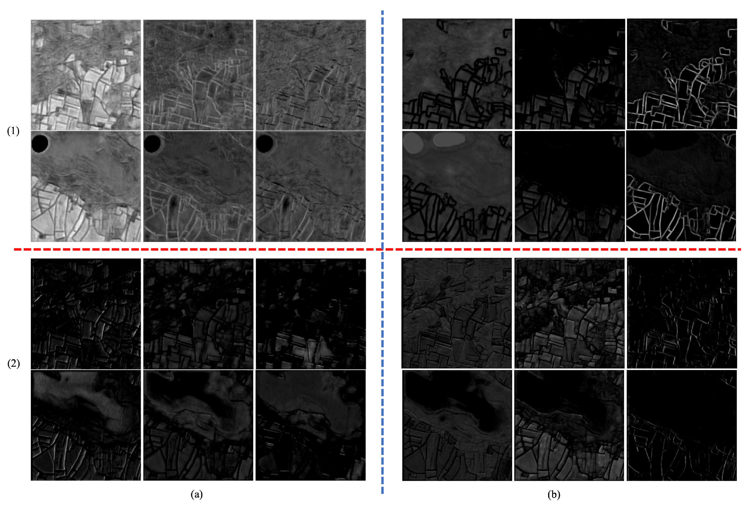
The analysis of the feature maps, as depicted in Figure 12, is highly important to demonstrate the distinctive characteristics introduced by the frequency attention mechanism in the FAUNet model. The visible contrast between the activation maps of FAUNet and those of the vanilla U-Net model validates the use of FAUNet for the parcel delineation framework.
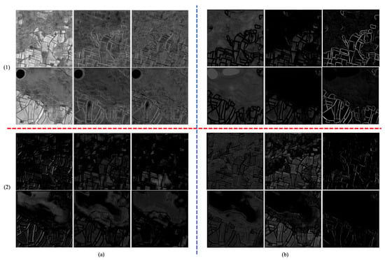
Figure 12.
U-Net and FAUNet feature map comparison. (1) FAUNet feature maps, (2) U-Net feature map, (a) third upscaling layer from the edge expanding path output, (b) fourth upscaling layer of the edge expanding path output.
In the context of the FAUNet architecture, the activation maps, as presented in (1) of the figure, emphasize the visible impact of the frequency attention gate. A pattern can be observed where each layer’s activation map exhibits a prominent improvement in the focus on edge-related information. This heightened attention to edges aligns perfectly with the fundamental objective of the frequency attention mechanism, which aims to equip the model with the capability to selectively focus on edge details within its learned representations. Consequently, the resulting feature maps provide a visual indication of the model’s sensitivity and responsiveness to edges within the image.
Conversely, the activation maps of the conventional U-Net architecture, as portrayed in part (2) of Figure 12, show distinctly different results. These activation maps follow closely the expected patterns characteristic of traditional convolutional neural network (CNN) designs. The absence of the frequency attention mechanism is reflected in the activation maps, which exhibit conventional convolution-based responses without the distinct emphasis on edge features. This conventional behavior is a consequence of the absence of the frequency attention gate.
Essentially, the analysis of the feature maps distinctly emphasizes the differing behaviors between FAUNet and the standard U-Net model. The activation maps of FAUNet reveal its ability to boost and emphasize edge-related information, effectively showcasing the intended impact of the frequency attention gate. At the same time, the activation maps of the standard U-Net model align with the usual behavior anticipated from a traditional CNN architecture. This further emphasizes the significant influence that the incorporation of the frequency attention gate has on the model’s hidden representations.
5. Discussion
In this study on boundary delineation, we propose an improved U-Net architecture that focuses on better detection of edge information. Central to this novel approach is the dual-pathway method, wherein one path handles the standard segmentation (extent path) and the other concentrates on edge delineation (edge path). The edge path contains a unique attention mechanism, which is informed by high-frequency details captured using high-pass filters. Specifically, these filters, designed to highlight rapid transitions such as edges, help generate attention maps through trainable convolution weights. This attention is applied before the up-sampling stages to ensure that the generated attention maps optimally influence the model’s predictions. Through this design, our U-Net variant FAUNet can efficiently “focus” on boundaries while concurrently performing standard segmentation tasks. The dual output, producing both an extent mask and an improved edge mask, leads to a more streamlined and simple post-processing step. FAUNet is built with boundary delineation in mind, and it performs accordingly.
In this study, a comprehensive evaluation of four prominent segmentation models: U-Net, ResUNet-a, BsiNet, SEANet, and FAUNet was performed. The comparison was based on two primary facets: pixel-based and object-based metrics. From the pixel-based perspective, as highlighted in Table 1, each model demonstrated specific strengths. U-Net achieved a satisfactory result, while ResUNet-a showcased an impressive overall accuracy. BsiNet, which was once considered state of the art until SEANet took that title, produced very good pixel-based and object-based numbers; it struck a good balance between over-segmentation and under-segmentation and maintained good pixel-based metrics while being the most efficient model in terms of complexity. SEANet emerged as a balanced candidate, with commendable recall and well-rounded figures across all metrics. However, FAUNet outperformed all of them, registering the highest values in precision, F1 score, and IoU. On the other hand, when evaluating the object-based metrics, Table 2 further demonstrates FAUNet’s superior performance. With the lowest errors in over-segmentation (OS) and under-segmentation (US) and a top-ranking F1 score at the object level (), FAUNet showed better results than the other models. SEANet came in second with consistent results, whereas U-Net and ResUNet-a struggled with higher OS and US values, indicating possible segmentation discrepancies. Drawing from the comprehensive analysis, it is clear that FAUNet outperforms the other evaluated models in both pixel- and object-based metrics. Its ability to strike a balance between precise boundary delineation and accurate segmentation positions it as a good candidate for applications demanding precise segmentation.
Lastly, in light of the ablation study findings, it is evident that the FAUNet model holds a distinct advantage over the vanilla U-Net model for edge detection within agricultural parcels. The superior edge mask precision and edge mask recall metrics of FAUNet underscore its efficacy in minimizing false positives and adeptly capturing the true edges. Moreover, the lower rates of over-segmentation and under-segmentation further highlight its proficiency. One key factor that really boosts FAUNet’s improved performance is how it uses the frequency attention mechanism. The contrasting feature map representations between FAUNet and the vanilla U-Net underscore the former’s heightened sensitivity to edge-related information. As agricultural parcel delineation demands precision, FAUNet’s increase in performance is clearly a result of its use of frequency attention gate. Moreover, this opens up an exciting opportunity to enhance edge detection techniques in this field. In the times ahead, researchers might harness the capabilities of FAUNet even further or explore its architecture more deeply to lay the groundwork for additional enhancements. Since our contributions can be summarized as the addition of the effective frequency attention gate as well as a simplified post-processing step, future studies can revolve around using this approach in more remote sensing applications that require more accurate edge detection such as road segmentation or building delineation.
However, there are specific areas where FAUNet exhibits certain shortcomings that require further refinement. Firstly, the dual-mask approach, despite its advantages, presents a challenge. Although FAUNet uses one mask fewer than certain other models, its reliance on two masks effectively doubles potential sources of error in comparison to a singular mask system. The inherent inaccuracies of each mask could compound, leading to magnified errors in the final boundary determination. Hence, while this approach facilitates post-processing, it also introduces complexities that might be prone to errors. Secondly, we must address the efficiency of FAUNet. Although in its current state FAUNet is less complex than other models, it could benefit from further streamlining and becoming more efficient. Thirdly, FAUNet falls short in comparison to other models when it comes to detecting all present parcels; this is a direct result of enhancing only the edge mask while neglecting the extent mask. Introducing an improvement to the extent mask can lead to a better recall value. Lastly, FAUNet may suffer from a lack of generalization to unseen distributions and new test areas. However, for future work, the emphasis on the high-frequency component in FAUNet might allow it to function akin to an unsupervised high-pass filter generating closed boundaries. By enhancing this aspect of FAUNet, it could become more adaptive to different locations and unseen imagery. In conclusion, FAUNet represents an incremental improvement over the state of the art when it comes to parcel boundary delineation. However, there remain exciting paths for future developments. As precision and efficiency become increasingly important in agricultural parcel delineation, models like FAUNet need to adapt and innovate to consistently meet and surpass the ever-evolving benchmarks.
Author Contributions
Conceptualization, B.A. and I.E.; methodology, B.A. and I.E.; software, B.A.; validation, B.A. and I.E.; formal analysis, I.E.; investigation, B.A. and I.E.; resources, B.A.; data curation, B.A. and I.E.; writing—original draft preparation, B.A. and I.E.; writing—review and editing, I.E.; visualization, B.A.; supervision, I.E.; project administration, I.E.; funding acquisition, B.A. All authors have read and agreed to the published version of the manuscript.
Funding
This research received no external funding.
Data Availability Statement
Data can be sourced from (https://collections.eurodatacube.com/, accessed on 1 January 2023). The implementation of FUANet will be shared at https://github.com/awadbahaa/FAUNet.
Conflicts of Interest
The authors declare no conflict of interest.
References
- Matton, N.; Sepulcre Canto, G.; Waldner, F.; Valero, S.; Morin, D.; Inglada, J.; Arias, M.; Bontemps, S.; Koetz, B.; Defourny, P. An automated method for annual cropland mapping along the season for various globally-distributed agrosystems using high spatial and temporal resolution time series. Remote Sens. 2015, 7, 13208–13232. [Google Scholar] [CrossRef]
- Belgiu, M.; Csillik, O. Sentinel-2 cropland mapping using pixel-based and object-based time-weighted dynamic time warping analysis. Remote Sens. Environ. 2018, 204, 509–523. [Google Scholar] [CrossRef]
- Wang, M.; Wang, J.; Cui, Y.; Liu, J.; Chen, L. Agricultural Field Boundary Delineation with Satellite Image Segmentation for High-Resolution Crop Mapping: A Case Study of Rice Paddy. Agronomy 2022, 12, 2342. [Google Scholar] [CrossRef]
- Yu, Q.; Shi, Y.; Tang, H.; Yang, P.; Xie, A.; Liu, B.; Wu, W. eFarm: A tool for better observing agricultural land systems. Sensors 2017, 17, 453. [Google Scholar] [CrossRef] [PubMed]
- Chen, Q.; Cao, W.; Shang, J.; Liu, J.; Liu, X. Superpixel-based cropland classification of SAR image with statistical texture and polarization features. IEEE Geosci. Remote Sens. Lett. 2021, 19, 4503005. [Google Scholar] [CrossRef]
- Li, H.; Zhang, C.; Zhang, Y.; Zhang, S.; Ding, X.; Atkinson, P.M. A Scale Sequence Object-based Convolutional Neural Network (SS-OCNN) for crop classification from fine spatial resolution remotely sensed imagery. Int. J. Digit. Earth 2021, 14, 1528–1546. [Google Scholar] [CrossRef]
- Graesser, J.; Ramankutty, N. Detection of cropland field parcels from Landsat imagery. Remote Sens. Environ. 2017, 201, 165–180. [Google Scholar] [CrossRef]
- Fetai, B.; Oštir, K.; Kosmatin Fras, M.; Lisec, A. Extraction of visible boundaries for cadastral mapping based on UAV imagery. Remote Sens. 2019, 11, 1510. [Google Scholar] [CrossRef]
- Cheng, T.; Ji, X.; Yang, G.; Zheng, H.; Ma, J.; Yao, X.; Zhu, Y.; Cao, W. DESTIN: A new method for delineating the boundaries of crop fields by fusing spatial and temporal information from WorldView and Planet satellite imagery. Comput. Electron. Agric. 2020, 178, 105787. [Google Scholar] [CrossRef]
- Xia, L.; Luo, J.; Sun, Y.; Yang, H. Deep extraction of cropland parcels from very high-resolution remotely sensed imagery. In Proceedings of the IEEE 2018 7th International Conference on Agro-Geoinformatics (Agro-Geoinformatics), Hangzhou, China, 6–9 August 2018; pp. 1–5. [Google Scholar]
- Garcia-Pedrero, A.; Lillo-Saavedra, M.; Rodriguez-Esparragon, D.; Gonzalo-Martin, C. Deep learning for automatic outlining agricultural parcels: Exploiting the land parcel identification system. IEEE Access 2019, 7, 158223–158236. [Google Scholar] [CrossRef]
- Diakogiannis, F.I.; Waldner, F.; Caccetta, P.; Wu, C. ResUNet-a: A deep learning framework for semantic segmentation of remotely sensed data. ISPRS J. Photogramm. Remote Sens. 2020, 162, 94–114. [Google Scholar] [CrossRef]
- Waldner, F.; Diakogiannis, F.I. Deep learning on edge: Extracting field boundaries from satellite images with a convolutional neural network. Remote Sens. Environ. 2020, 245, 111741. [Google Scholar] [CrossRef]
- Zhang, H.; Liu, M.; Wang, Y.; Shang, J.; Liu, X.; Li, B.; Song, A.; Li, Q. Automated delineation of agricultural field boundaries from Sentinel-2 images using recurrent residual U-Net. Int. J. Appl. Earth Obs. Geoinf. 2021, 105, 102557. [Google Scholar] [CrossRef]
- Waldner, F.; Diakogiannis, F.I.; Batchelor, K.; Ciccotosto-Camp, M.; Cooper-Williams, E.; Herrmann, C.; Mata, G.; Toovey, A. Detect, consolidate, delineate: Scalable mapping of field boundaries using satellite images. Remote Sens. 2021, 13, 2197. [Google Scholar] [CrossRef]
- Jong, M.; Guan, K.; Wang, S.; Huang, Y.; Peng, B. Improving field boundary delineation in ResUNets via adversarial deep learning. Int. J. Appl. Earth Obs. Geoinf. 2022, 112, 102877. [Google Scholar] [CrossRef]
- Lu, R.; Wang, N.; Zhang, Y.; Lin, Y.; Wu, W.; Shi, Z. Extraction of agricultural fields via dasfnet with dual attention mechanism and multi-scale feature fusion in south xinjiang, china. Remote Sens. 2022, 14, 2253. [Google Scholar] [CrossRef]
- Xu, L.; Yang, P.; Yu, J.; Peng, F.; Xu, J.; Song, S.; Wu, Y. Extraction of cropland field parcels with high resolution remote sensing using multi-task learning. Eur. J. Remote Sens. 2023, 56, 2181874. [Google Scholar] [CrossRef]
- Long, J.; Li, M.; Wang, X.; Stein, A. Delineation of agricultural fields using multi-task BsiNet from high-resolution satellite images. Int. J. Appl. Earth Obs. Geoinf. 2022, 112, 102871. [Google Scholar] [CrossRef]
- Li, M.; Long, J.; Stein, A.; Wang, X. Using a semantic edge-aware multi-task neural network to delineate agricultural parcels from remote sensing images. ISPRS J. Photogramm. Remote Sens. 2023, 200, 24–40. [Google Scholar] [CrossRef]
- Ronneberger, O.; Fischer, P.; Brox, T. U-net: Convolutional networks for biomedical image segmentation. In Proceedings of the Medical Image Computing and Computer-Assisted Intervention—MICCAI 2015: 18th International Conference, Munich, Germany, 5–9 October 2015; Proceedings, Part III 18. Springer: Berlin/Heidelberg, Germany, 2015; pp. 234–241. [Google Scholar]
- He, K.; Zhang, X.; Ren, S.; Sun, J. Identity mappings in deep residual networks. In Proceedings of the Computer Vision—ECCV 2016: 14th European Conference, Amsterdam, The Netherlands, 11–14 October 2016; Proceedings, Part IV 14. Springer: Berlin/Heidelberg, Germany, 2016; pp. 630–645. [Google Scholar]
- Chen, L.C.; Papandreou, G.; Kokkinos, I.; Murphy, K.; Yuille, A.L. Deeplab: Semantic image segmentation with deep convolutional nets, atrous convolution, and fully connected crfs. IEEE Trans. Pattern Anal. Mach. Intell. 2017, 40, 834–848. [Google Scholar] [CrossRef]
- Zhao, H.; Shi, J.; Qi, X.; Wang, X.; Jia, J. Pyramid scene parsing network. In Proceedings of the IEEE Conference on Computer Vision and Pattern Recognition, Honolulu, HI, USA, 21–26 July 2017; pp. 2881–2890. [Google Scholar]
- Oktay, O.; Schlemper, J.; Folgoc, L.L.; Lee, M.; Heinrich, M.; Misawa, K.; Mori, K.; McDonagh, S.; Hammerla, N.Y.; Kainz, B.; et al. Attention u-net: Learning where to look for the pancreas. arXiv 2018, arXiv:1804.03999. [Google Scholar]
- Schlemper, J.; Oktay, O.; Chen, L.; Matthew, J.; Knight, C.; Kainz, B.; Glocker, B.; Rueckert, D. Attention-gated networks for improving ultrasound scan plane detection. arXiv 2018, arXiv:1804.05338. [Google Scholar]
- Wang, F.; Jiang, M.; Qian, C.; Yang, S.; Li, C.; Zhang, H.; Wang, X.; Tang, X. Residual attention network for image classification. In Proceedings of the IEEE Conference on Computer Vision and Pattern Recognition, Honolulu, HI, USA, 21–26 July 2017; pp. 3156–3164. [Google Scholar]
- Shen, T.; Zhou, T.; Long, G.; Jiang, J.; Pan, S.; Zhang, C. Disan: Directional self-attention network for rnn/cnn-free language understanding. In Proceedings of the AAAI Conference on Artificial Intelligence, New Orleans, LA, USA, 2–7 February 2018; Volume 32. [Google Scholar]
- Wang, X.; Girshick, R.; Gupta, A.; He, K. Non-local neural networks. In Proceedings of the IEEE Conference on Computer Vision and Pattern Recognition, Salt Lake City, UT, USA, 18–22 June 2018; pp. 7794–7803. [Google Scholar]
- Mnih, V.; Heess, N.; Graves, A.; Kavukcuoglu, K. Recurrent models of visual attention. In Proceedings of the Advances in Neural Information Processing Systems, Montreal, QC, Canada, 8–13 December 2014; Volume 27. [Google Scholar]
- Tong, X.; Wei, J.; Sun, B.; Su, S.; Zuo, Z.; Wu, P. ASCU-Net: Attention gate, spatial and channel attention u-net for skin lesion segmentation. Diagnostics 2021, 11, 501. [Google Scholar] [CrossRef] [PubMed]
- Nodirov, J.; Abdusalomov, A.B.; Whangbo, T.K. Attention 3D U-Net with Multiple Skip Connections for Segmentation of Brain Tumor Images. Sensors 2022, 22, 6501. [Google Scholar] [CrossRef]
- Deng, W.; Shi, Q.; Li, J. Attention-gate-based encoder–decoder network for automatical building extraction. IEEE J. Sel. Top. Appl. Earth Obs. Remote Sens. 2021, 14, 2611–2620. [Google Scholar] [CrossRef]
- Susladkar, O.; Deshmukh, G.; Nag, S.; Mantravadi, A.; Makwana, D.; Ravichandran, S.; Chavhan, G.H.; Mohan, C.K.; Mittal, S. ClarifyNet: A high-pass and low-pass filtering based CNN for single image dehazing. J. Syst. Archit. 2022, 132, 102736. [Google Scholar] [CrossRef]
- Bertasius, G.; Shi, J.; Torresani, L. Semantic segmentation with boundary neural fields. In Proceedings of the IEEE Conference on Computer Vision and Pattern Recognition, Las Vegas, NV, USA, 27–30 June 2016; pp. 3602–3610. [Google Scholar]
- Marmanis, D.; Schindler, K.; Wegner, J.D.; Galliani, S.; Datcu, M.; Stilla, U. Classification with an edge: Improving semantic image segmentation with boundary detection. ISPRS J. Photogramm. Remote Sens. 2018, 135, 158–172. [Google Scholar] [CrossRef]
- Papasaika-Hanusch, H. Digital Image Processing Using Matlab; Institute of Geodesy and Photogrammetry, ETH Zurich: Zürich, Switzerland, 1967; Volume 63. [Google Scholar]
- Sudre, C.H.; Li, W.; Vercauteren, T.; Ourselin, S.; Jorge Cardoso, M. Generalised dice overlap as a deep learning loss function for highly unbalanced segmentations. In Proceedings of the Deep Learning in Medical Image Analysis and Multimodal Learning for Clinical Decision Support: Third International Workshop (DLMIA 2017), and 7th International Workshop (ML-CDS 2017), Held in Conjunction with MICCAI 2017, Québec City, QC, Canada, 14 September 2017; Proceedings 3. Springer: Berlin/Heidelberg, Germany, 2017; pp. 240–248. [Google Scholar]
- Milletari, F.; Navab, N.; Ahmadi, S.A. V-net: Fully convolutional neural networks for volumetric medical image segmentation. In Proceedings of the IEEE 2016 4th International Conference on 3D Vision (3DV), Stanford, CA, USA, 25–28 October 2016; pp. 565–571. [Google Scholar]
- Yeung, M.; Sala, E.; Schönlieb, C.B.; Rundo, L. Unified focal loss: Generalising dice and cross entropy-based losses to handle class imbalanced medical image segmentation. Comput. Med. Imaging Graph. 2022, 95, 102026. [Google Scholar] [CrossRef]
- Persello, C.; Bruzzone, L. A novel protocol for accuracy assessment in classification of very high resolution images. IEEE Trans. Geosci. Remote Sens. 2009, 48, 1232–1244. [Google Scholar] [CrossRef]
- Rieke, C. Deep Learning for Instance Segmentation of Agricultural Fields. Master’s Thesis, Friedrich-Schiller-University, Jena, Germany, 2017. [Google Scholar]
- Karasiak, N.; Dejoux, J.F.; Monteil, C.; Sheeren, D. Spatial dependence between training and test sets: Another pitfall of classification accuracy assessment in remote sensing. Mach. Learn. 2022, 111, 2715–2740. [Google Scholar] [CrossRef]
Disclaimer/Publisher’s Note: The statements, opinions and data contained in all publications are solely those of the individual author(s) and contributor(s) and not of MDPI and/or the editor(s). MDPI and/or the editor(s) disclaim responsibility for any injury to people or property resulting from any ideas, methods, instructions or products referred to in the content. |
© 2023 by the authors. Licensee MDPI, Basel, Switzerland. This article is an open access article distributed under the terms and conditions of the Creative Commons Attribution (CC BY) license (https://creativecommons.org/licenses/by/4.0/).