A General Relative Radiometric Correction Method for Vignetting Noise Drift

Abstract

Due to the limitation of the number of sensor pixels, optical splicing is commonly used to improve the imaging width of remote sensing satellites, and this optical stitching can cause vignetting in the image data of adjacent sensors. The weak energy, low signal-to-noise ratio, and poor response stability of vignetting are key factors that restrict the relative radiometric correction of optical splicing remote satellites. This paper proposes a stability analysis method and a relative radiometric correction method for vignetting. First, we analyzed the stability of the response and the noise impact of vignetting. Massive data from the Jilin-1 GF03D satellites was used to analyze the stability of the response using the vignetting stability analysis method. Secondly, the data on the deep sea during nighttime (DDSN) of Jilin-1 GF03D satellites was used to obtain the characteristics of the sensors’ noise. Thirdly, by building a noise drift model, we calculated the coefficient of the noise drift according to its characteristics. Using the coefficient to eliminate the noise drift of each pixel in vignetting can improve the response stability of vignetting. The average response stability increased by 37.64% by this method. Finally, the automatic relative radiometric correction method was completed through histogram matching. Furthermore, we proposed color aberration metrics (CAMs) to evaluate the multi-spectral images after relative radiometric correction, and massive data from the 16 satellites of Jilin-1 GF03D was used to verify the effectiveness and generality. The experimental results show that the average CAM of the images increased by 15.97% using the proposed method compared to the traditional method.

1. Introduction

Optical remote sensing satellites have the advantages of being easy to monitor and interpret by the human eye and are widely used in fields such as land survey, agriculture, forestry, and environmental protection. With the development of remote sensing satellite application technology, optical remote sensing satellites with large widths and high resolutions have become a trend [1]. However, the manufacturing of large-sized image sensors is complex and costly [2,3]. Therefore, scholars suggested concatenating multiple sensors to meet the current requirements for resolution and width [4,5]. There are generally two types of sensor splicing technology: mechanical splicing and optical splicing.

Mechanical splicing is arranging multiple image sensors closely on a single satellite, which is currently adopted by many large-width remote sensing satellites. The advantage is that the camera optical system using mechanical splicing is relatively simple, but the drawback is the high satellite manufacturing costs, launch costs, and the possible existence of a splicing gap [6,7,8]. In this case, in order to obtain a large field of view, optical splicing is gradually adopted by more and more optical remote sensing satellites. Optical splicing is the process of dividing the field of view into different spatial positions through optical methods, receiving them with multiple image sensors, and then splicing the images received by the image sensors to obtain a large and wide image. Compared to mechanical splicing, optical splicing camera systems have a compact structure and significant advantages in volume, weight, and technology [9,10,11]. They have become the main developing direction of sensor splicing technology, and the advantages of remote-sensing satellite cameras are becoming increasingly apparent.

Due to the presence of a splitter in the optical path of an optical splicing remote sensing satellite, a portion of the light cannot be projected onto the sensor through the reflector, resulting in energy loss and low response in the partial image. This phenomenon is called vignetting [12]. Because of this, the signal-to-noise ratio is also low [13,14]. Therefore, it is challenging to develop relative radiometric correction methods of optical splicing remote sensing satellites for vignetting images. Traditional relative radiometric correction methods are mainly divided into two methods: calibration and statistical methods.

The laboratory calibration method employs an integrating sphere as a uniform light source to image at different radiance levels [15,16,17]. This method calibrates the response disparities, utilizing multiple samples, between pixels in both vignetting and non-vignetting, thereby generating the laboratory relative radiometric calibration coefficient. LI Jing et al. [18] conducted a radiometric calibration of a photographic camera with a composite plane array CCD in a laboratory setting. The advantage of this method is that the accuracy of the radiometric calibration coefficient is high, which can better smooth out the responding differences between pixels of vignetting and non-vignetting. However, the disadvantage is that the coefficient effectiveness is reduced as the sensor decays [19]. Moving on to another method, the uniform field calibration method capitalizes on data from low-, medium-, and high-response typical uniform object features (e.g., oceans, deserts, glaciers) to ascertain the coefficient. Dennis L. Helder [20] has strengthened the long-term radiometric stability monitoring of visible and near-infrared Earth observation sensors by employing uniform fields, such as the Sonoran Desert, Sahara, and Middle Eastern Desert regions. The advantage of this method is that it lowers the prerequisite for specific sensors and satellites, thus eliminating the need for massive data. The drawback is that with the increase in the width of remote sensing satellites and the expansion of the image coverage area, the number of large-area uniform fields that meet the requirements decreases [21]. Also, the yaw calibration method has morphed into a laudable on-orbit relative radiometric calibration technique [22]. This method ensures the focal plane detector array’s alignment parallel to the imaging direction, enabling each detector to traverse the same ground stretch, thus receiving an identical amount of light. Chaochao and Chen [23] applied the yaw calibration method, introducing a side-slither data-based vignetting correction technique for a high-resolution spaceborne camera with an optical focal plane assembly. The yaw calibration method facilitates relative radiometric calibration for focal plane pixels, and its high timeliness and ability to capture more gray-level responses in a single imaging enhance the universality of the relative radiometric calibration coefficient. However, this method requires a high level of satellite attitude adjustment capability and stability, a challenge often faced by traditional satellites to achieve stable yaw imaging capabilities [24].

Statistical methods mainly include histogram matching and moment matching methods [25,26]. Histogram matching is used to improve the signal-to-noise ratio by adding the response of corresponding points of vignetting [27]. Shapira D. [28] proposed a new method that finds such a mapping in an optimal manner under various histogram distance measures. The method can find a single monotonic mapping between multiple pairs of histograms, such that the mapping will satisfy all pairs simultaneously. The moment matching method assumes that the radiometric distribution of each sensor for ground object detection is balanced, and the gain between sensors is linearly correlated with the drift value [29]. Jia Li [30] proposed a novel destriping method based on adaptive material matching (MAM). The pixels are matched by thresholding their vertical gradients and leveraging both the inner-stripe gradient feature (ISGF) and neighbor-stripe geometry feature (NSGF). The positive of statistical methods is that good correction coefficients can be obtained based on historical satellite data, and they have no requirement on the capability of satellites. The shortcoming is that the pixel response characteristics have changed, and their correction effect is extremely poor.

To solve the problem of correcting the vignetting of optical remote sensing satellites, Yongkun Liu [31] proposed a general relative radiometric correction method to correct vignetting (correction of vignetting of multiple CCDs). The entropy and IDM threshold are used to select the uniform image block. The improved least-squares method, ridge regression, is used to fit vignetting correction parameters, and the global optimization parameters model is established according to the difference of overlap pixels between each CCD. Newton’s method is used to calculate the global optimal correction parameters. However, this method relies on the response stability of vignetting or a high signal-to-noise ratio. Once the image data do not meet the above two requirements, the relative radiometric correction effect will be greatly reduced. With the continuous attenuation of satellite sensors, changes in the response of vignetting are inevitable.

In summary, the above relative radiometric correction methods do not provide special image processing for vignetting and cannot solve the problem of vignetting effectively. To overcome these difficulties, we proposed a general relative radiometric method by building a model to improve the stability of the response of vignetting, thereby improving the quality of relative radiometric correction.

Our key contributions in this paper are:

• A general relative radiometric correction method for vignetting is proposed, including a vignetting stability analysis method, data on the deep sea during nighttime (DDSN), a noise drift model for vignetting, and histogram matching, which can effectively improve the relative radiometric correction effect;
• A vignetting stability analysis method is proposed by calculating the variation in response differences of corresponding points to explore the stability and effect of vignetting noise;
• The noise drift model for vignetting is built using the DDSN of Jilin-1 GF03D satellites. The imaging time and the mean of each pixel of vignetting are used to calculate the coefficient of the model. The coefficient is used to eliminate the noise and noise drift, and the experiments show that the average response stability increased by 37.64% using the method;
• Histogram matching is used to correct the image after the noise drift model for vignetting;
• The results of the comparison of 56,843 images from the Jilin-1 GF03D satellites show that the average improvement rate of color aberration metrics (CAMs) of images after correction in this paper is 15.97%, which is significantly better than the existing method and verifies the generality of the proposed method.

2. Methods

This paper aims to solve the problem of relative radiometric correction of the vignetting of an optical splicing remote sensing satellite. First, a vignetting stability analysis method is proposed to explore the stability of the characteristics of response and the noise of vignetting. Then, we build a noise drift model in vignetting using the DDSN and complete a relative radiometric correction method. The workflow of this method is as follows:

• Analyze the stability of the energy and the noise effect of vignetting using the vignetting stability analysis method;
• Obtain the noise of vignetting by the DDSN of Jilin-1 GF03D satellites;
• Build a noise drift model for vignetting based on the DDSN;
• Histogram matching is used to complete a relative radiometric correction method after the noise drift model correction.

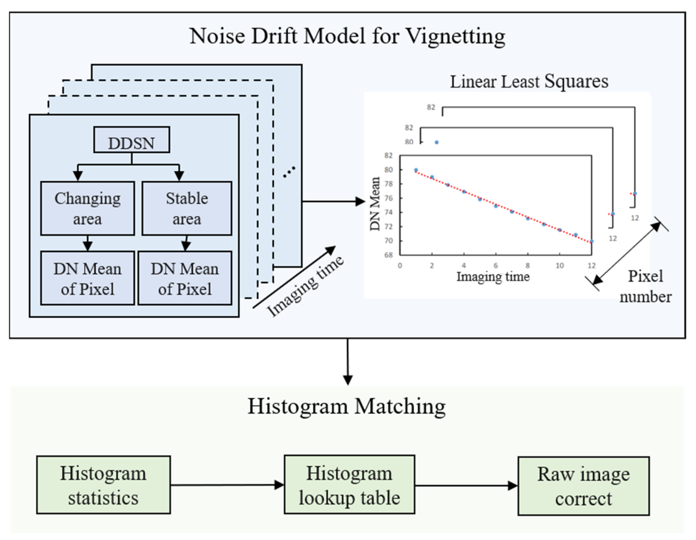
The workflow of this method is shown in Figure 1. First, vignetting is divided into stable and changing areas based on the DDSN, this is to analyze the stability of the response. Then, build a noise drift model for vignetting based on the DDSN and generate the noise drift coefficient of the vignetting using linear least squares to fit the imaging time and the response of each pixel. We find that it is not necessary to distinguish between changing area and stable area, so all the coefficients are used to calculate the noise drift uniformly. Finally, histogram matching is used to correct the image, which is pre-corrected by the noise drift model for vignetting.

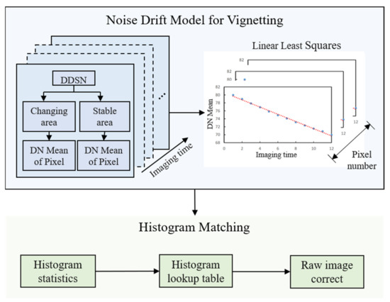
Figure 1. Workflow of the noise drift model for vignetting.

2.1. The Vignetting Stability Analysis Method

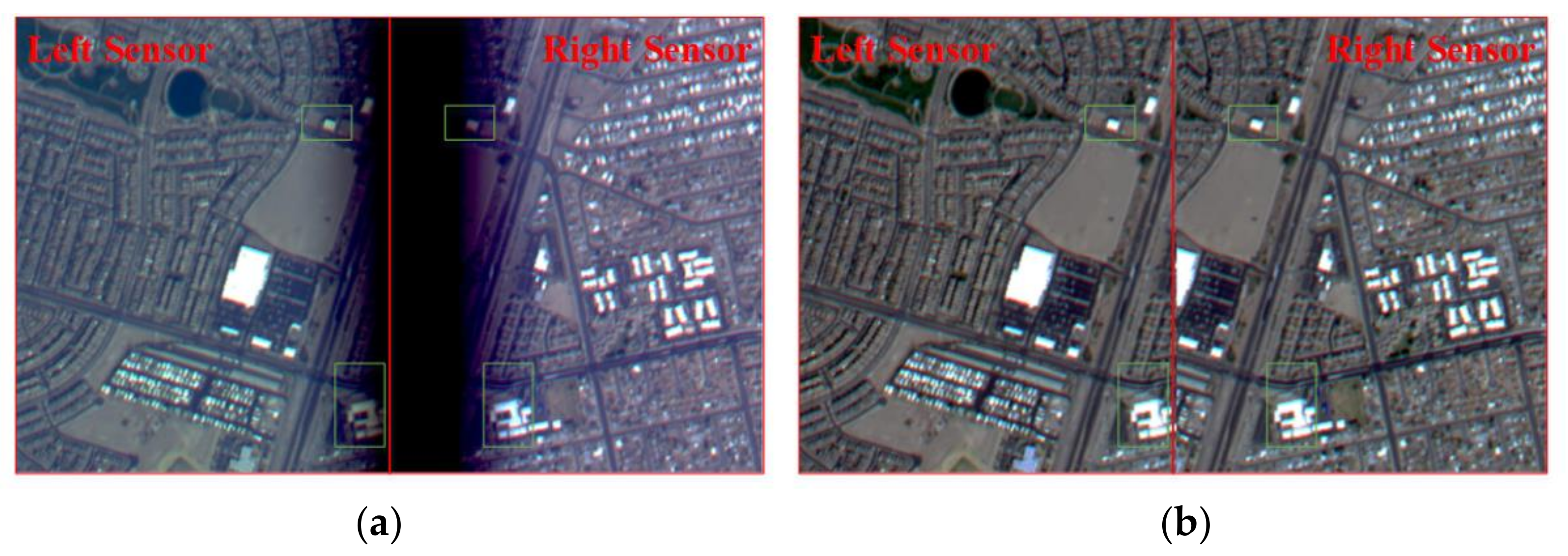
The pixels of the vignetting of adjacent sensors will show the same object features during the imaging of optical splicing remote sensing satellites, as shown in Figure 2. The width of the images is 4000, and the width of each sensor is 2000. This is to better demonstrate the difference in the object features between vignetting and non-vignetting in each sensor, as well as the response differences. This can be used to calculate the energy distribution of vignetting. The energy and noise characteristics of adjacent sensors are different, and the energy of the corresponding points is also completely inconsistent. In general, the response of the corresponding points of vignetting is relatively stable at different imaging times and tasks when the noise is stabilized. Conversely, the response points are unstable with violently changing noises. The energy distribution of the vignetting is calculated by the response ratio of the corresponding points. The response ratio can be calculated according to Formula (1):

$$E_i=\frac{{{\displaystyle \sum }}_{j=1}^{H}D{N}_{\left(L,i,j\right)}}{{{\displaystyle \sum }}_{j=1}^{H}D{N}_{\left(R,i,j\right)}},$$

(1)

where $E_i$ is the energy ratio of the $i$th corresponding point of vignetting. $H$ is the image height. $D{N}_{\left(L,i,j\right)}$ and $D{N}_{\left(R,i,j\right)}$ are the corresponding points. $D{N}_{\left(L,i,j\right)}$ is the $i$th pixel of the vignetting of the left sensor. $D{N}_{\left(R,i,j\right)}$ is the $i$th pixel of the vignetting of the right sensor.

Figure 2. Vignetting image: (a) raw image; (b) corrected image.

The energy stability of vignetting can be calculated using the response ratio standard deviation of the corresponding points in different scenes. The formula for the calculation is as follows:

$$EST{D}_i=\sqrt{\frac{{{\displaystyle \sum }}_{n=1}^N{\left(E_{\left(i,n\right)}-{\overline{E}}_i\right)}^2}{N},}$$

(2)

where $EST{D}_i$ is the energy stability and $E_{\left(i,n\right)}$ is the energy ratio of the $i$th corresponding point in the $n$th image. ${\overline{E}}_i$ is the mean of the $i$th corresponding point energy ratio. $N$ is the number of scenes.

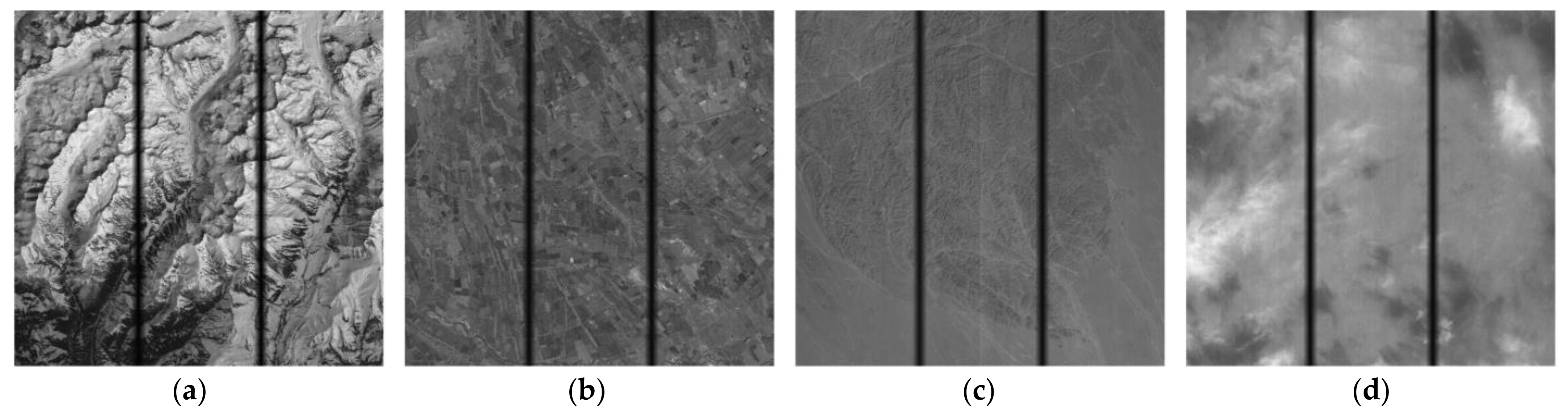
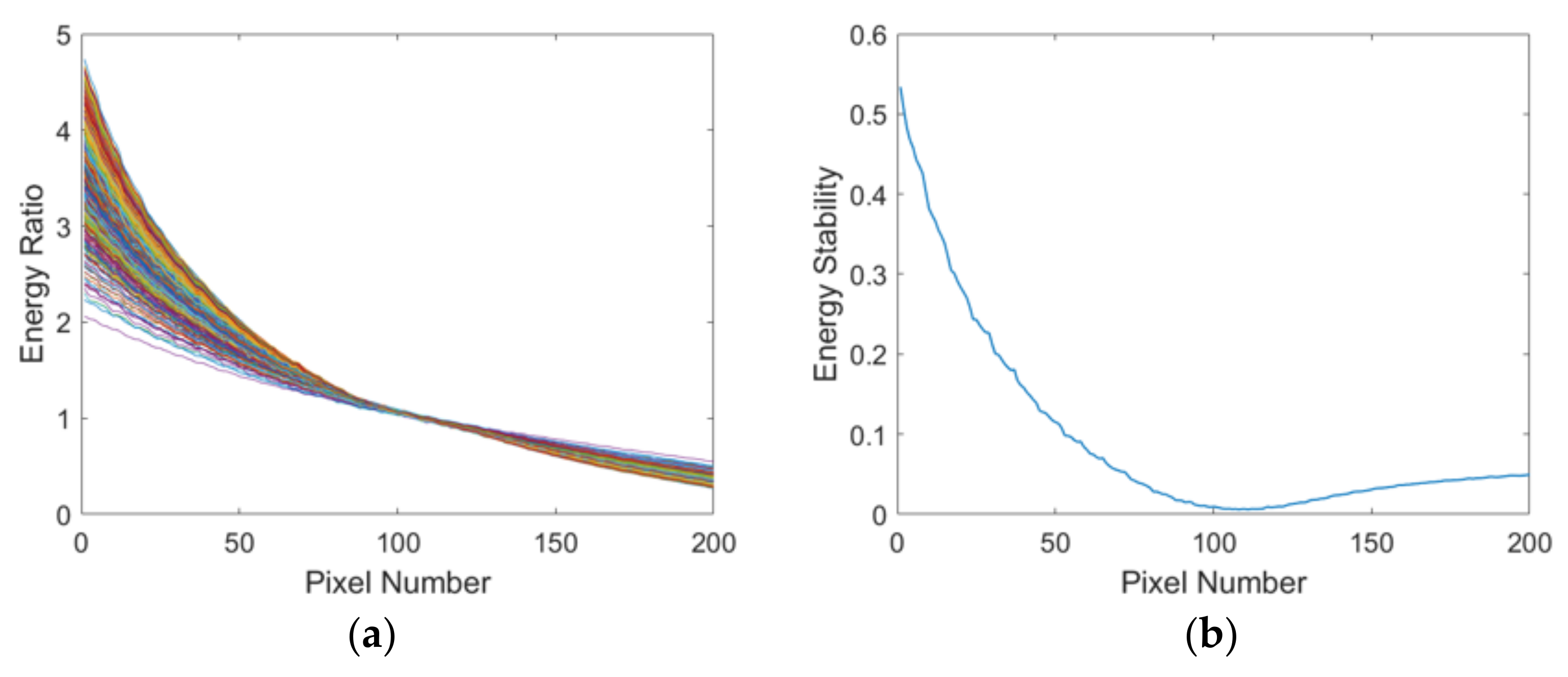
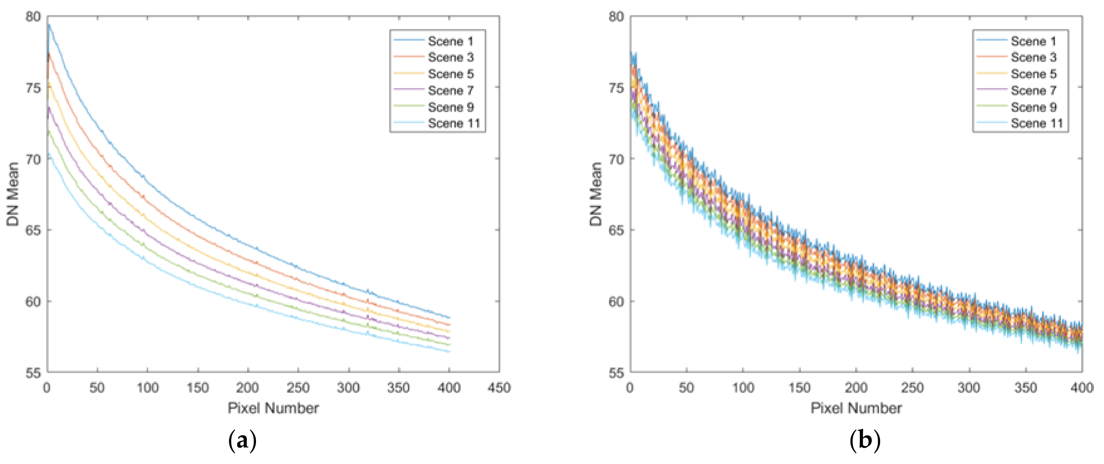
The Jilin-1 GF03D28 satellite captured 56 images at (83.517°E, 43.557°N) for 130 s at 2:56:42 Beijing time, 1 April 2023. There are only 4 typical object features among them, such as mountain, city, farmland, and cloud, which is a sample that is shown in Figure 3. The number of sensors in the Jilin-1 GF03D satellite is 3, and the width of the vignetting in each sensor is about 400 pixels. The energy ratio and the energy stability of each pixel of vignetting are calculated using the data. The number of curves is 56, and they all come from the above data. The energy stability of each corresponding point is not consistent, as shown in Figure 4. In addition, due to the extremely low response at the edge of vignetting, the energy ratio is extremely high. To make the energy ratio and energy standard deviation of the corresponding points in the figure clearer, this paper only selects 200 pixels in the middle of vignetting as samples for plotting.

Figure 3. Object features: (a) mountain; (b) city; (c) farmland; (d) cloud.

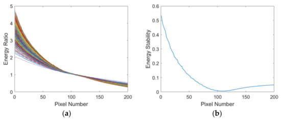
Figure 4. Energy ratio and energy standard deviation of the corresponding points of 56 images in 130 s. (a) Energy ratio of the corresponding points of vignetting; (b) energy stability of each corresponding point of vignetting.

The energy stability of the corresponding points at the center of vignetting is better than others, and the edge corresponding point is poor. The energy stability of each corresponding point is also inconsistent. This indicates that the energy stability is affected by the noise of the sensors, and each pixel of vignetting has independent noise; the noise also changes with the imaging time. This change has affected the stability of the pixel and made relative radiometric correction difficult.

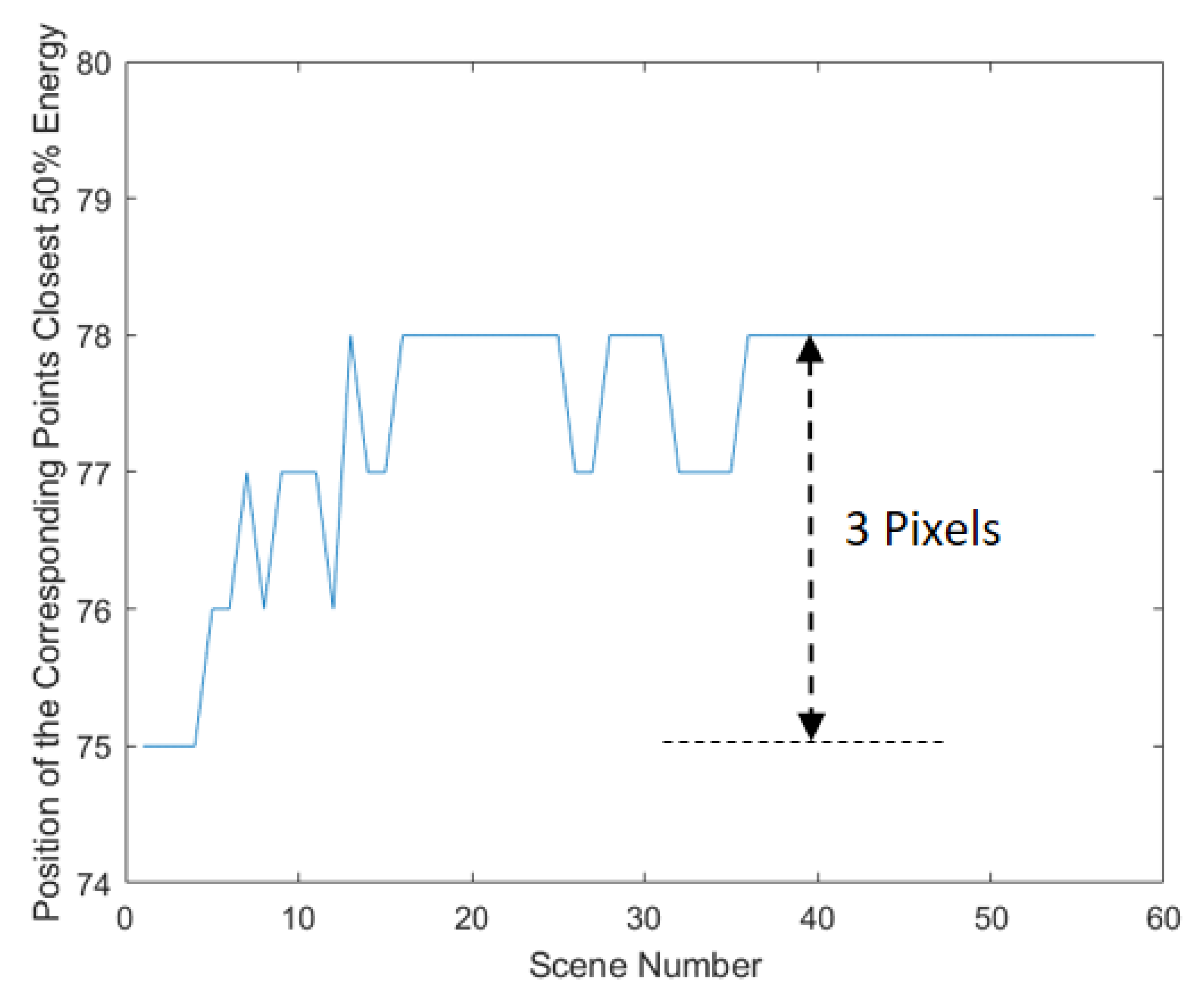
Due to the design of the optical system for the optical splicing of remote sensing satellites, the pixels near the edge of the sensor obtain low response and a poor signal-to-noise ratio [32]. The corresponding points closest to the center of the vignetting of the two sensors have the highest signal-to-noise ratio, and the effect of noise is minimal. The energy ratio can be calculated by every pixel in every scene. The position of the pixel with the closest energy ratio of 1 is the corresponding point with the closest 50% energy in each scene. So, the position of the corresponding points with the closest 50% energy also can prove the fluctuation of the noise of vignetting, which is shown in Figure 5. It can be seen that the position changes with the imaging time. The maximum deviation of the positions is 3 pixels.

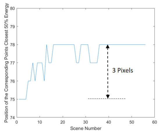
Figure 5. Position of the corresponding points with the closest 50% energy.

In summary, the method proves that the fluctuation of the noise of the sensors affects energy stability. The imaging method of the Jilin-1 GF03D satellites is Push–Broom, and the columnar response of the image is generated from the same pixel, so it has the same characteristics of response and is not related to the object features. According to the position of the corresponding points with the closest 50% energy, the position changes with the scene number, and the change in scene number represents the change in imaging time. In addition, the energy ratio and energy standard deviation of each corresponding point are not consistent. So, the noise of each pixel is independent and changes with the imaging time. It limits the validity of the relative radiometric correction of vignetting. For this reason, this paper will analyze the response of the noise of vignetting using the DDSN of the Jilin-1 GF03D satellite.

2.2. Data on the Deep Sea during Nighttime (DDSN)

To obtain the noise of vignetting, we used the Jilin-1 GF03D12 satellite to image the DDSN of the Earth at 6:10:55 Beijing time on 15 February 2023, with the imaging center point at (3.6914°E, 3.988°N). The parameters of the satellite are shown in Table 1. PAN is the panchromatic band, MSS1 is the blue band, MSS2 is the green band, MSS3 is the red band, and MSS4 is the near-infrared band. The integration level and gain are the imaging parameters of the sensor. The sensor increases the energy obtained and amplifies the response by adjusting them. We use different imaging parameters based on different imaging conditions to obtain a better response image.

Table 1. Parameters of the sensor imaging DDSN.

Band	Integral Level	Gain	Scenes
PAN	64	2	12
MSS1	16	2
MSS2	12	2
MSS3	8	3
MSS4	8	4

To avoid the impact of clouds and sea waves on the validity of the data, we used the column means of each pixel to test the effectiveness. Formula (3) is as follows:

$${\overline{DN}}_{\left(i,m\right)}=\frac{{{\displaystyle \sum }}_{j=0}^{n}D{N}_{\left(i,j,m\right)}}{n},$$

(3)

where ${\overline{DN}}_{\left(i,m\right)}$ is the column mean of the $i$th pixel in the $m$th scene, and $n$ is the scene height, $D{N}_{\left(i,j,m\right)}$ is the response of $j$th row in the $i$th column of the $m$th scene.

Both valid and invalid data, the latter caused by sea waves, are presented in Figure 6. Ideally, as shown in Figure 6a, while each pixel’s response may vary, the differences between adjacent pixels should be stable and exhibit minimal fluctuations. Contrary to this expectation, Figure 6b demonstrates that adjacent pixels have significantly different responses and show considerable fluctuations.

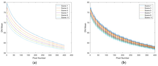
Figure 6. The column mean of the DDSN: (a) valid image, the response difference of each pixel between scenes is stable and fluctuates less; (b) invalid image, the response difference of each pixel between scenes is significant and fluctuates more.

2.3. The Noise Drift Model for Vignetting

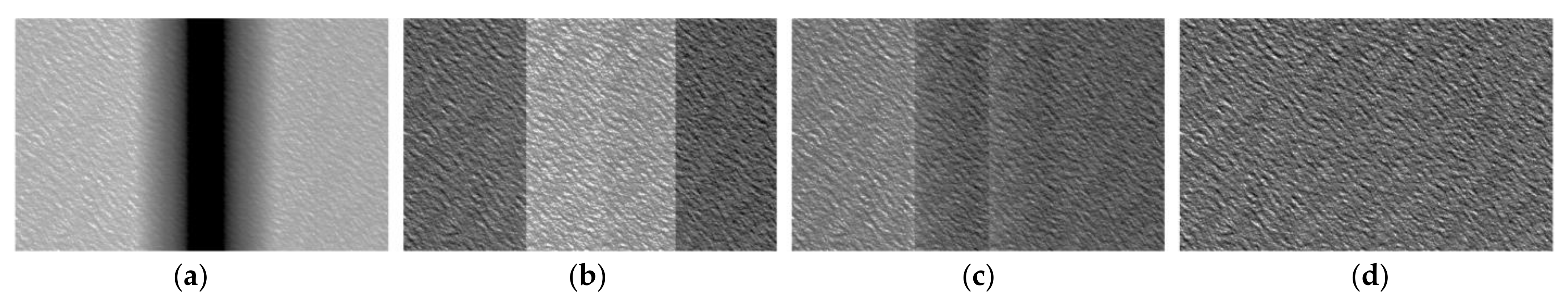
We segregate vignetting into “Stable Area” and “Changing Area” based on the DDSN response difference of pixels between each scene. Pixels with a difference of less than 1 DN are allocated to the “Stable Area”, while others are designated to the “Changing Area”. As shown in Figure 7, the response changes of each pixel in the changing area are significant, exhibiting inconsistent noise characteristics, whereas the response changes in the stable area are minimal, exhibiting consistent noise characteristics.

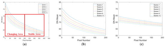
Figure 7. Vignetting division: (a) vignetting division method; (b) changing Area; (c) stable Area.

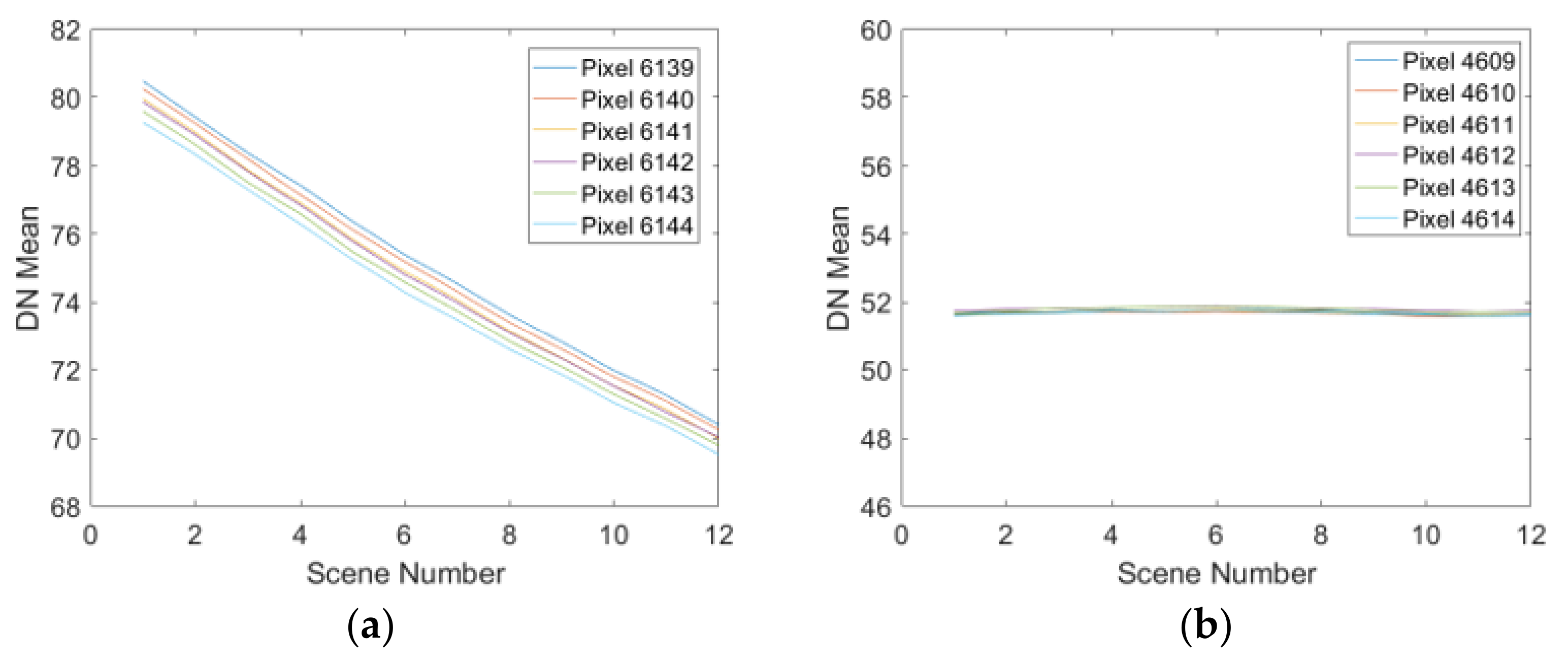
Six pixels from both stable and changing areas are randomly selected to explore the characteristics of noise. The fluctuation of noise is shown in Figure 8. Each curve in the changing and stable area represents the column mean of each pixel. The change in noise in the changing area is significant, and each curve shows a basic linear trend, as shown in Figure 8a. The change in noise in the stable area is small and irregular, as shown in Figure 8b. Due to the response in the DDSN representing the noise of each pixel, we correlate the response with the imaging time, and then we sort the images using the imaging time. The first scene is the earliest imaged image, and the last scene is the latest imaged image, and we find that each pixel basically has a linear characteristic based on Figure 8. The valid images are selected by relying on the rules shown in Figure 6 and Formula (3). So, the noise characteristics of each pixel of vignetting is not consistent. It leads to a decrease in the stability of the effective response, which also proves the conclusion of the vignetting stability analysis method.

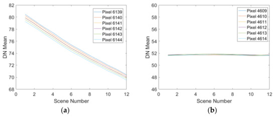
Figure 8. Response of each pixel. (a) Changing Area. (b) Stable Area.

We build a noise drift model for vignetting using the DDSN of the Jilin-1 GF03D satellite. The noise of each pixel is calculated by the mean of each pixel of vignetting. Formula (4) as follows:

$$B{N}_i=\frac{{{\displaystyle \sum }}_{j=0}^{H}D{N}_{\left(i,j\right)}}{H},$$

(4)

where $D{N}_{\left(i,j\right)}$ is the response of the $j$th row and $i$th pixel of vignetting. $H$ is the total rows of each scene of the DDSN.

The noise drift changes with the imaging time, so it can be calculated by the difference between the mean of the noise and real-time noise. Formula (5) is as follows:

$$N{D}_{\left(i,m\right)}={\overline{DN}}_{\left(i,m\right)}-B{N}_i,$$

(5)

where $N{D}_{\left(i,m\right)}$ is the noise drift of the $i$th pixel and ${\overline{DN}}_{\left(i,m\right)}$ is the column mean of the $i$th pixel in the $m$th scene.

The coefficient of the noise drift model for vignetting can be calculated by the imaging time and noise drift. The imaging time is calculated by Formula (6):

$$\Delta T=T_{i+1}-T_i,$$

(6)

where $\Delta T$ is the imaging time between the $i$th scene and $\left(i+1\right)$th scene. $T_i$ is the imaging time of the middle row of the $i$th scene data. We linearly fit the noise drift and the imaging time in Formula (7):

$$f\left(k_i,b_i\right)=profit\left(N{D}_i,\Delta T_i,M\right),$$

(7)

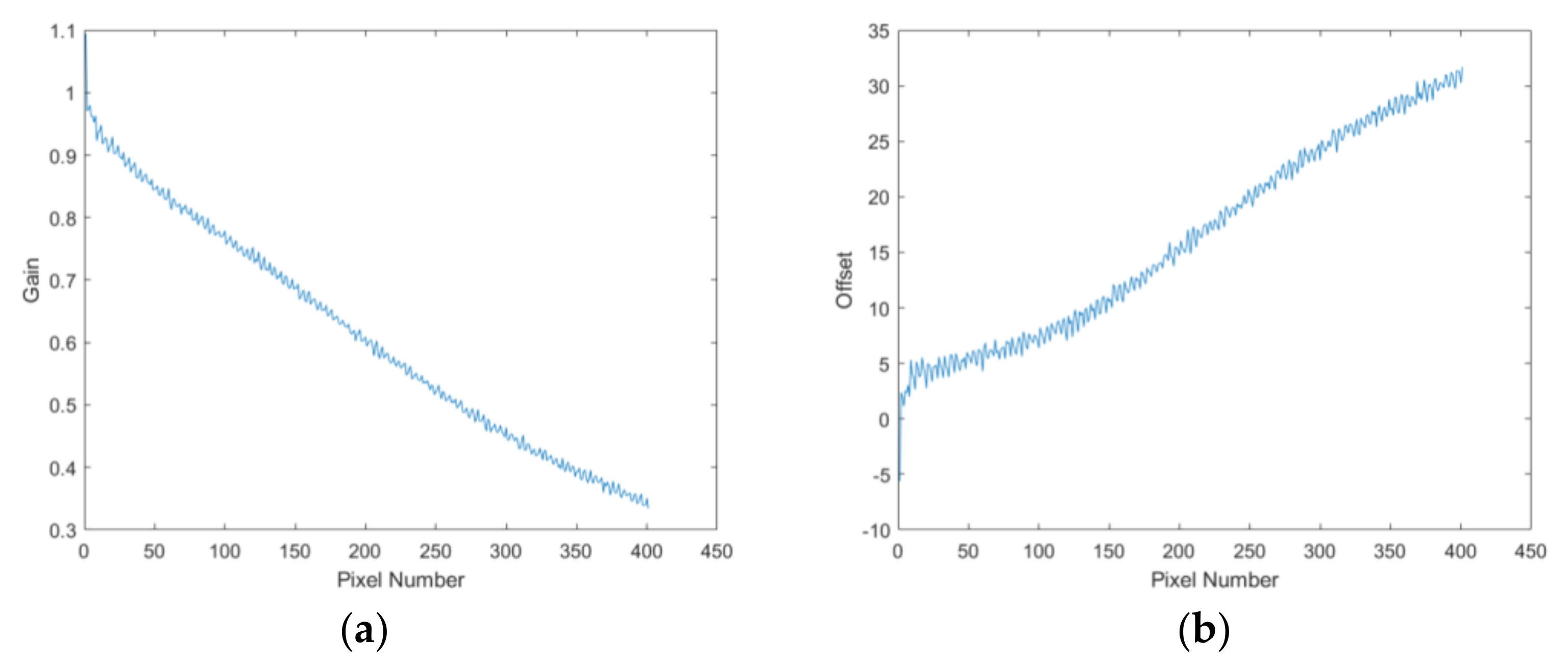
where $f\left(k_i,b_i\right)$ is the coefficient of the noise drift of the $i$th pixel. $M$ is the total amount of scenes. $profit$ is the linear least-squares method. We can use the auxiliary data recorded in real-time imaging by the satellite to obtain the imaging time corresponding to the image of each pixel. The coefficient consists of gain and offset, which is $k_i \mathrm{and} b_i$. We use $k_i$ (gain) to describe the noise drift by the imaging time and use $b_i$ (offset) to describe the bottom noise of each pixel. The gain and offset of the coefficient of the noise drift are shown in Figure 9.

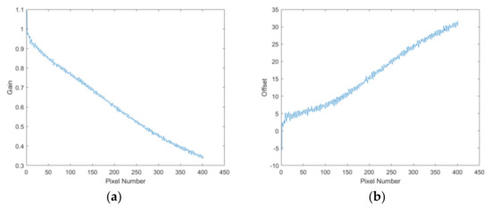
Figure 9. Coefficients of each pixel: (a) gain; (b) offset.

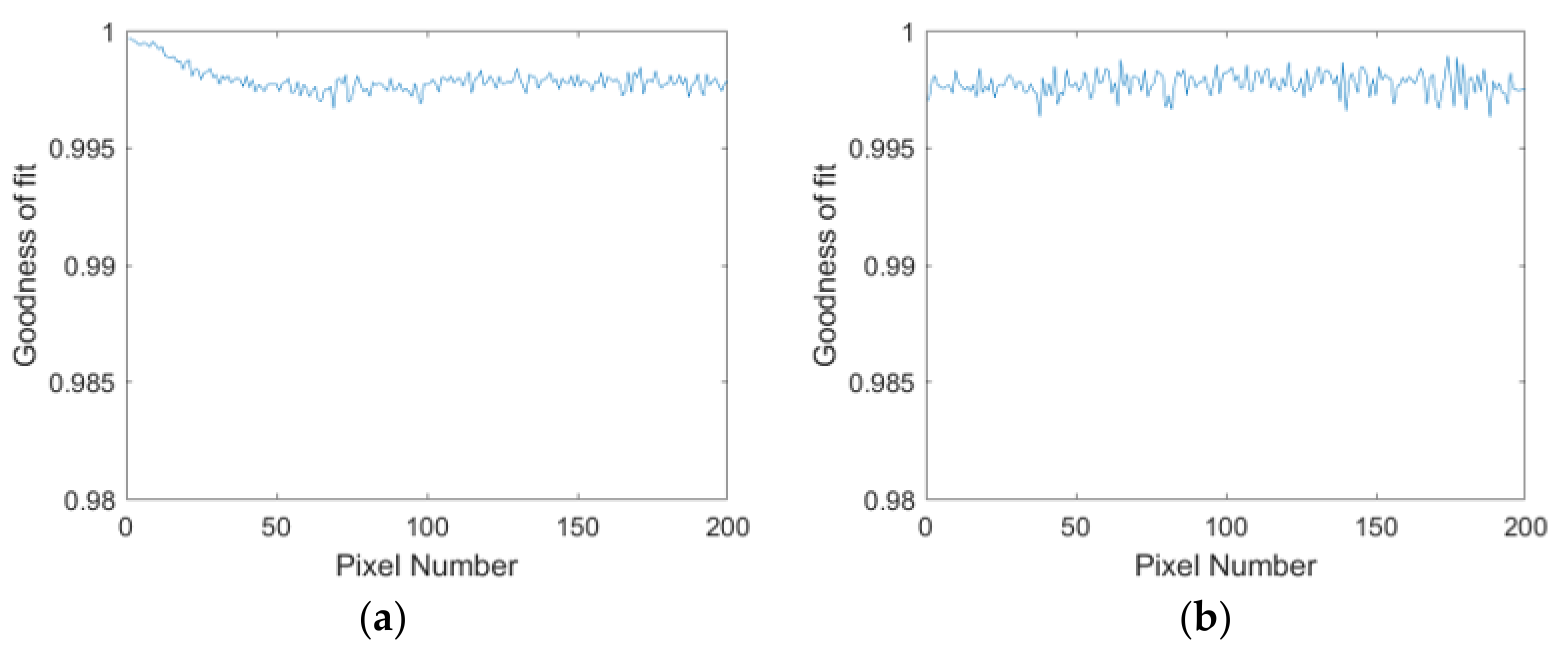
We use the goodness of fit to evaluate the effectiveness of the coefficients in Formula (8):

$$R^2=\frac{{{\displaystyle \sum }}_{i=1}^n{({\widehat{y}}_i-\overline{y})}^2}{{{\displaystyle \sum }}_{i=1}^n{\left(y_i-\overline{y}\right)}^2}$$

(8)

where $R^2$ is the goodness of fit. $n$ is the total number of fitting data. ${\widehat{y}}_i$ is the $i$th calculation result after fitting. $\overline{y}$ is the mean of the fitting data. The goodness of fit of the stable and changing area is shown in Figure 10. The average of the goodness of fit in the changing area is higher than the stable area. The validity of the model is proved by the high goodness of fit.

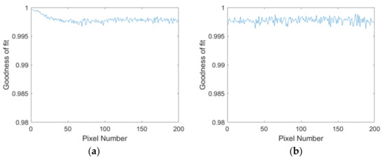
Figure 10. Goodness of fit: (a) changing area; (b) stable area.

Although the goodness of fit is lower in the stable area, the gain is a minimum. The differences in the offset of each pixel are also relatively consistent, and the imaging time is gradual. We considered that the goodness of fit would not have a significant impact on the noise of the stable area. So, we did not distinguish between stable and changing areas and used the coefficient to correct the data uniformly. The coefficients are used to eliminate the noise of the vignetting, which can improve the stability of vignetting and effectively improve the relative radiometric correction effect of images.

2.4. The Relative Radiometric Correction Method

We first obtain the noise drift using the DDSN of the Jilin-1 GF03D satellite. Secondly, we build the noise drift model for vignetting and calculate the coefficient to eliminate vignetting noise and the impact of noise changes on images. Thirdly, we add the response of the corresponding points of vignetting. Finally, we use histogram matching to complete a relative radiometric correction method. The method is as follows.

Step One: Calculate the noise drift of each pixel of vignetting using Formula (9):

$$N_{\left(i,j\right)}=k_i\ast T_j+b_i,$$

(9)

where $N_{\left(i,j\right)}$ is the noise of the $j$th row and $i$th pixel. $T_j$ is the imaging time between the $j$th and 1st row images. The valid response of each pixel of vignetting is calculated using Formula (10):

$$D{N}_{\left(i,j\right)}^{\prime }=D{N}_{\left(i,j\right)}-N_{\left(i,j\right)},$$

(10)

where $D{N}_{\left(i,j\right)}^{\prime }$ is the response of the $j$th row and $i$th pixel after the noise drift model for vignetting. $D{N}_{\left(i,j\right)}$ is the original response of the $j$th row and $i$th pixel.

Step Two: Add the response of the corresponding points of vignetting, which is corrected by the noise drift model for vignetting in Formula (11):

$$D{N}_{\left(i,j\right)}^{″}=D{N}_{\left(L,i,j\right)}^{\prime }+D{N}_{\left(R,i,j\right)}^{\prime },$$

(11)

where $D{N}_{\left(i,j\right)}^{″}$ is the response of the $j$th row and $i$th pixel after adding the response of the corresponding point. $D{N}_{\left(L,i,j\right)}^{\prime }$ and $D{N}_{\left(R,i,j\right)}^{\prime }$ are the corresponding points.

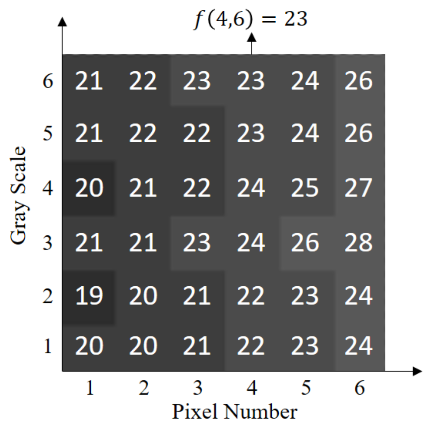
Step Three: The histogram matching method is used for the relative radiometric calibration to generate a histogram lookup table, as shown in Figure 11. The horizontal coordinates are the pixel numbers, and the horizontal coordinates are the gray scales.

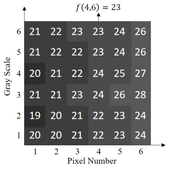
Figure 11. Histogram lookup table. The DN of the 4th pixel is 6, and the corrected DN is $f\left(4,6\right)$ = 23.

Step Four: The relative radiometric correction method is completed using the histogram lookup table.

2.5. Accuracy Assessment Index

The root-mean-square deviation of the mean line (RA) [31] and streaking metrics (SMs) [32] are used to evaluate the results of relative radiometric correction, and the root-mean-square of vignetting and non-vignetting (RSVN) is used to evaluate the consistency between vignetting and non-vignetting. The CAM is used to evaluate the results of the relative radiometric correction of multi-spectral data.

2.5.1. Root-Mean-Square Deviation of the Mean Line (RA)

The imaging method of the Jilin-1 GF03D satellites is Push–Broom, and the columnar response of the image is generated from the same pixel, so it has the same characteristics of response. The accuracy of the relative radiometric correction is influenced by the noise present in each pixel. In the same uniform scene, a lower RA value, indicating higher image uniformity, also implies higher relative radiometric correction accuracy, signifying effective noise elimination. This relationship underpins the utilization of RA as an indicator of relative radiometric correction accuracy in our analysis. RA can evaluate the relative radiometric accuracy, which is shown in Formula (12):

$$RA=\frac{\sqrt{\frac{{{\displaystyle \sum }}_n{\left(mea{n}_i-\overline{mean}\right)}^2}{n}}}{\overline{mean}}\ast 100\%,$$

(12)

where $\overline{mean}$ is the mean for the image, $mea{n}_i$ is the column mean of $i$th pixel, and $n$ is the width of the image.

2.5.2. Streaking Metrics (SMs)

The verified images are evenly divided into small image blocks. The size of every block is 400 × 400, and the selected area is in vignetting. SMs are used to detect the uniformity of blocks, which is shown in Formula (13):

$$S{M}_i=\frac{{{\displaystyle \sum }}_{j=1}^n\frac{\left|mea{n}_i-\overline{mean}\right|}{mea{n}_i+\overline{mean}}}{n}\ast 100\%,$$

(13)

where $mea{n}_i$ is the mean of the $j$th column mean of the image block, $\overline{mean}$ is the mean of the image block, and $n$ is the width of the image block. The lower the streaking metrics are, the more uniform the image is.

2.5.3. Root-Mean-Square of Vignetting and Non-Vignetting (RSVN)

The object features of adjacent pixels should be similar. This paper uses RSVN to evaluate the consistency of response between vignetting and non-vignetting in uniform images. It is shown in Formula (14):

$$RSVN=\sqrt{\frac{{{\displaystyle \sum }}_{i=0}^H{{\displaystyle \sum }}_{j=0}^W{(D{N}_V{}_{\left(i,j\right)}-D{N}_{nV}{}_{\left(i,j\right)})}^2}{W\ast H}},$$

(14)

where $W$ is the image width, $H$ is the image height, and $D{N}_V{}_{\left(i,j\right)}$ is the response of the $j$th row and $i$th pixel of vignetting. $D{N}_{nV}{}_{\left(i,j\right)}$ is the response of the $j$th row and $i$th pixel in non-vignetting. RSVN should be calculated by the corrected image. The smaller RSVN, the higher the accuracy of the response between vignetting and the non-vignetting.

2.5.4. Color Aberration Metrics (CAMs)

We propose CAMs to evaluate the multi-spectral images after relative radiometric correction. The CAM is used to measure the uniformity of the column response of multi-spectral data. First, histogram equalization is used by multi-spectral data. Then, convert the image to LAB color space. Finally, the CAM is calculated by the difference of the column mean in the LAB color space. It is shown in Formulas (15) and (16):

$$La{b}_i=\frac{{\overline{mean}}_{i+1}-{\overline{mean}}_i}{{\overline{mean}}_{max}},$$

(15)

$$CAM=\frac{{{\displaystyle \sum }}_{i=0}^W\frac{\left|La{b}_i-\overline{Lab}\right|}{La{b}_{max}}}{W}\ast \mathrm{10,000},$$

(16)

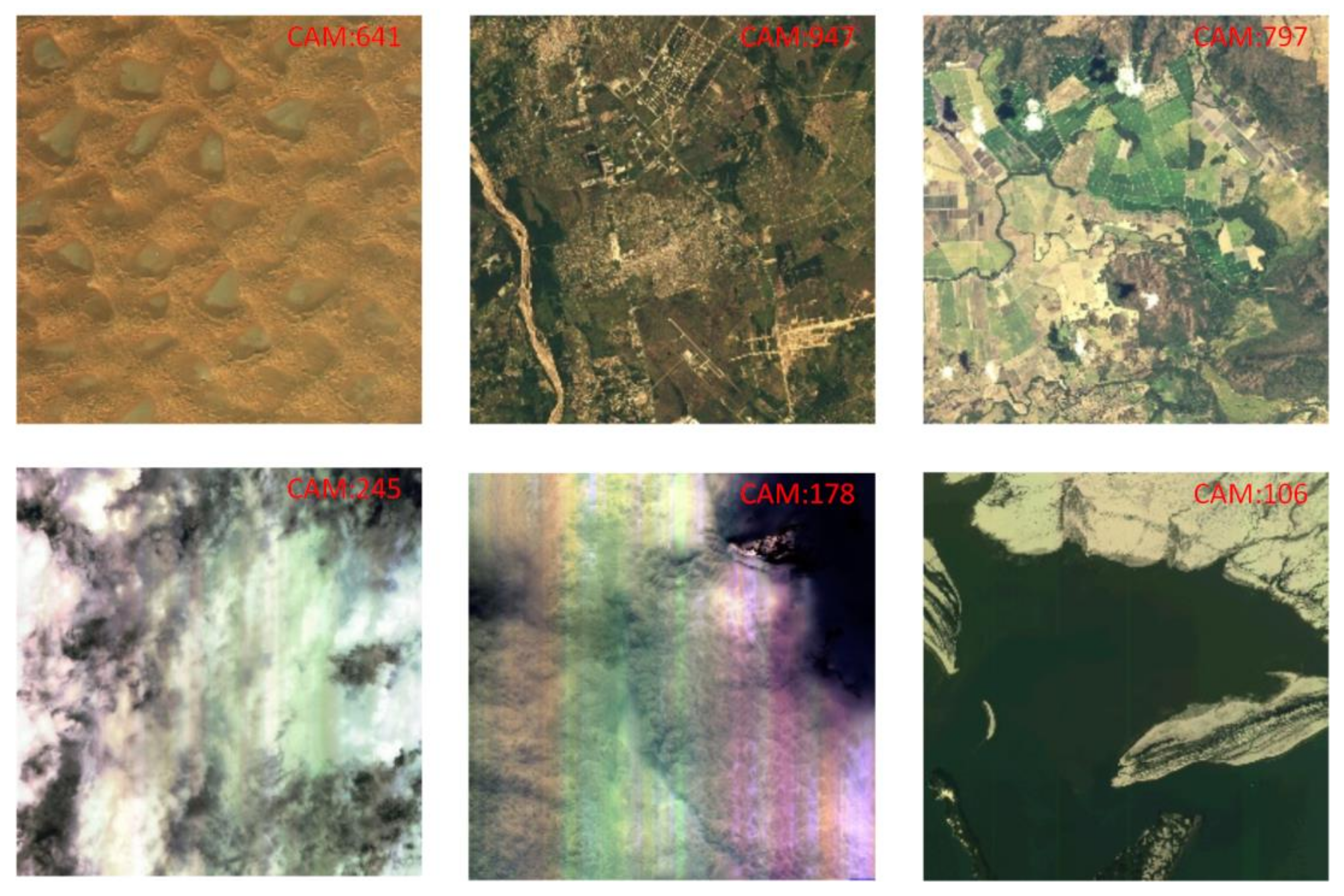
where $La{b}_i$ is the relative column mean of the $i$th pixel in LAB color space. ${\overline{mean}}_i$ is the column mean of the $i$th pixel in the LAB color space. ${\overline{mean}}_{max}$ is the maximal value of the image. $\overline{Lab}$ is the average of the relative column mean. $La{b}_{max}$ is the maximal value of the relative column mean in the image. $W$ is the image width. The experiments show that there is no chromatic aberration in multi-spectral images when CAMs are greater than 600; the results are shown in Figure 12.

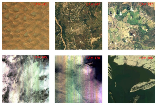
Figure 12. CAM results. The CAM of the first row of images is all greater than 600, which is good without color aberration. The CAM of the second row of images is all below 600, which shows significant color aberration.

3. Results

Experiment Setup

First, we use the sample from Section 2.1 to analyze the effectiveness of the vignetting stability analysis method. Second, 1031 imaging tasks and 15,927 images from the Jilin-1 GF03D28 satellite are used to validate the generality of the method. Third, the coefficient of the noise drift model for vignetting is calculated by the DDSN of 16 satellites of Jilin-1 GF03D. Fourth, five types of object features (water, deserts, cities, vegetation, and snow) are used as the visible sample set to compare the results of the methods, and three types of object features (water, vegetation, and desert) are used as a quantitative sample set to compare with relative radiometric correction methods. Finally, 56,843 images from the 16 satellites of Jilin-1 GF03D were used to prove the generality of the proposed method.

4. Discussion

4.1. Evaluation of the Stability of Vignetting

The evaluation of vignetting stability constitutes a critical aspect of this research. In this section, experiments are designed to validate the effectiveness and generality of the proposed noise drift model for vignetting.

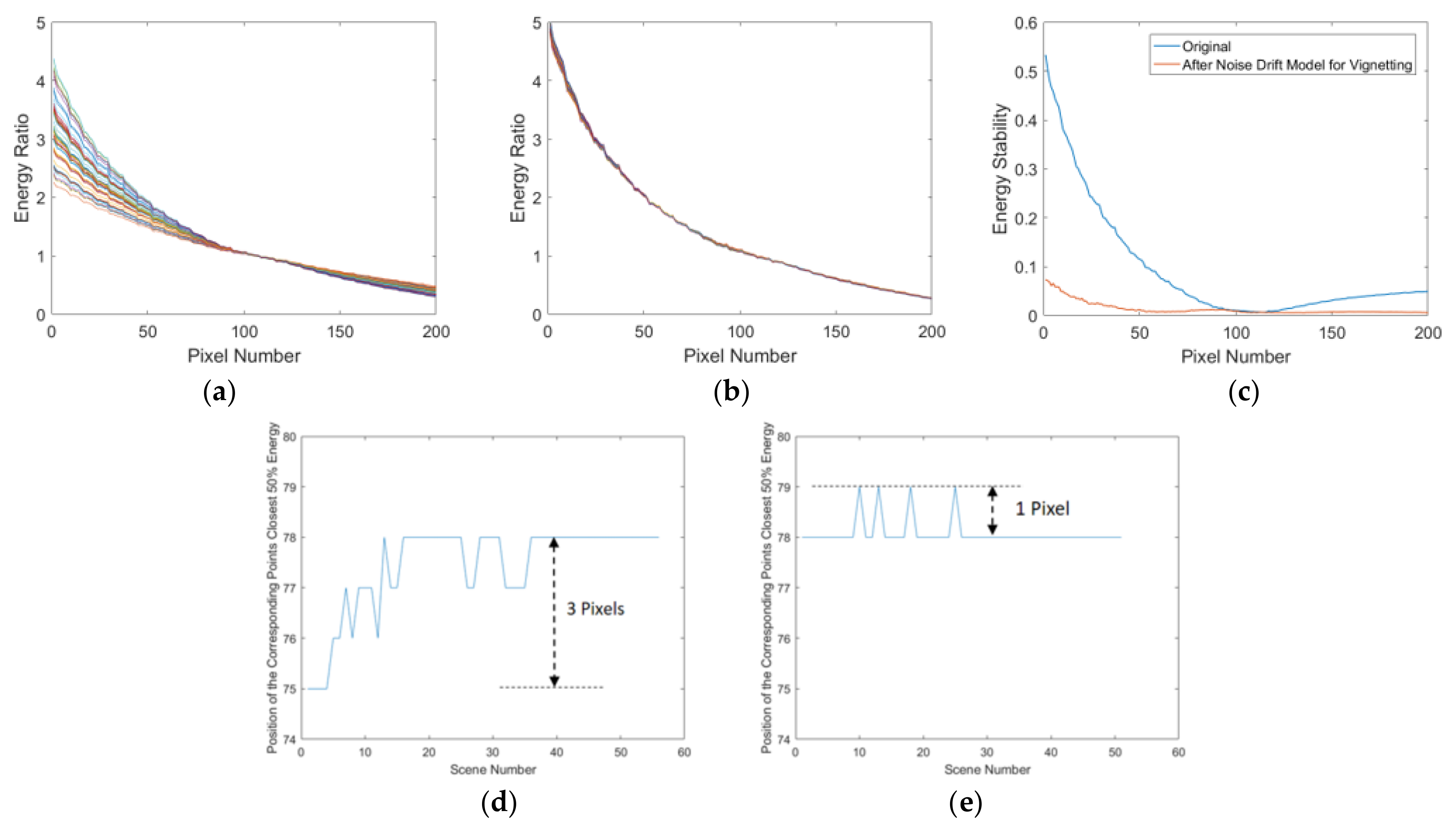
Initially, an experiment is designed to validate the effectiveness, employing the sample set elucidated in Section 2.1. As depicted in Figure 13, upon the application of the noise drift model for vignetting, a significant enhancement in the response stability of each pixel is observed, with an average of 51.50%. Moreover, the maximum deviation is optimized from three pixels to one pixel.

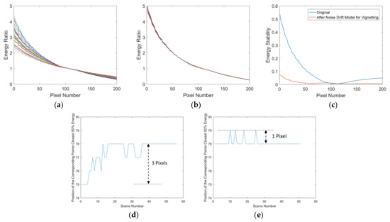
Figure 13. Evaluation of the vignetting stability analysis method using 56 images from Section 2.1. (a) Energy ratio before correction. (b) Energy ratio after correction using the noise drift model. (c) Response stability improvement for each corresponding point in the vignetting area, which shows an average of 51.50%. (d) Position before correction, with a maximum deviation of three pixels. (e) Position after correction, with a maximum deviation reduced to one pixel.

Furthermore, an experiment is designed to validate the generality of the method. Figure 14 presents a comparative experiment of vignetting stability analysis using a dataset comprising 15,927 images captured during 1031 imaging tasks by the Jilin-1 GF03D28 satellite from 1 February 2023 to 8 April 2023. It is imperative to emphasize that the images analyzed represent standard Push–Broom data, not the DDSN images. The results indicate that on one hand, the range of improvement in the energy standard deviation is an average of 37.64%. On the other hand, the maximum deviation is optimized from eight pixels to four pixels. These findings validate the generality of the noise drift model for vignetting correction across various imaging conditions and further verify its effectiveness.

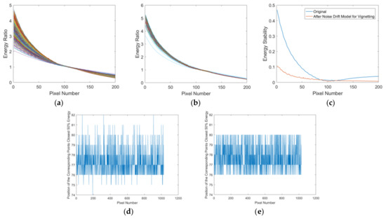
Figure 14. Evaluation of the vignetting stability analysis method using 15,927 images from 1031 imaging tasks by the Jilin-1 GF03D28 satellite (1 February 2023–8 April 2023)—non-DDSN data. (a) Energy ratio before correction. (b) Energy ratio after correction using the noise drift model. (c) Response stability improvement for each corresponding point in the vignetting, which shows an average of 37.64%. (d) Position before correction, with a maximum deviation of eight pixels. (e) Position after correction, with a maximum deviation reduced to four pixels.

4.2. Evaluation of Relative Radiometric Correction

We used the DDSN of 16 satellites of Jilin-1 GF03D as the calibration set to calculate the coefficient of the noise drift model for vignetting. The information is shown in Table 2. The minimum goodness of fit is shown in column 6, which is all higher than 0.95. The above results prove the effectiveness and generality of the noise drift model for vignetting.

Table 2. Information of the DDSN set of the Jilin-1 GF03D satellites.

Satellite	Imaging Time	Longitude	Latitude	Scene	Minimum Goodness of Fit
JL1GF03D01	2023-01-17	−17.9957	10.3161	13	0.9984
JL1GF03D03	2023-01-17	49.1638	29.1192	12	0.9962
JL1GF03D05	2023-01-13	96.9982	15.8312	12	0.9975
JL1GF03D07	2023-01-17	50.2294	28.0700	13	0.9972
JL1GF03D11	2022-11-28	40.122	17.9956	13	0.9971
JL1GF03D12	2022-11-17	5.9106	42.3907	13	0.9976
JL1GF03D13	2022-12-30	34.8815	26.7517	12	0.9915
JL1GF03D14	2023-01-13	35.6616	43.8903	12	0.9870
JL1GF03D15	2023-01-13	40.1879	42.0227	12	0.9972
JL1GF03D16	2023-01-13	11.6455	−27.7515	12	0.9887
JL1GF03D17	2023-01-13	34.8815	26.7517	12	0.9953
JL1GF03D18	2023-01-14	7.1630	42.6434	13	0.9968
JL1GF03D27	2022-12-30	50.2294	28.0700	13	0.9922
JL1GF03D28	2022-12-30	36.8701	43.9123	13	0.9978
JL1GF03D29	2023-01-17	35.8593	25.3234	13	0.9971
JL1GF03D30	2023-01-17	36.8701	43.9123	13	0.9510

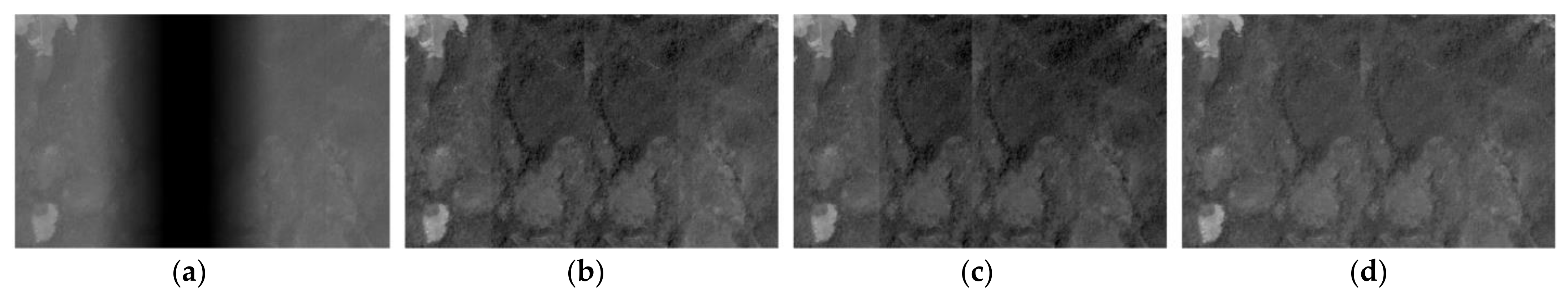
In this paper, histogram matching and correction of vignetting and chromatic aberration of multiple CCDs [31] are compared with the proposed method. Five types of object features (water, vegetation, cities, deserts, and snow) from Jilin-1 GF03D12, which are panchromatic bands with sizes of 800 × 600, are used to evaluate the results of the relative radiometric methods. The original and corrected images are shown in Figure 15, Figure 16, Figure 17, Figure 18 and Figure 19.

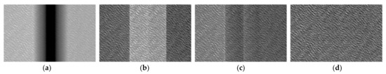
Figure 15. Raw and corrected images of the water. (a) Raw image; (b) corrected using histogram matching; (c) corrected using correction of the vignetting of multiple CCDs; (d) corrected using the proposed method.

Figure 16. Raw and corrected images of the vegetation. (a) Raw image; (b) corrected using histogram matching; (c) corrected using correction of the vignetting of multiple CCDs; (d) corrected using the proposed method.

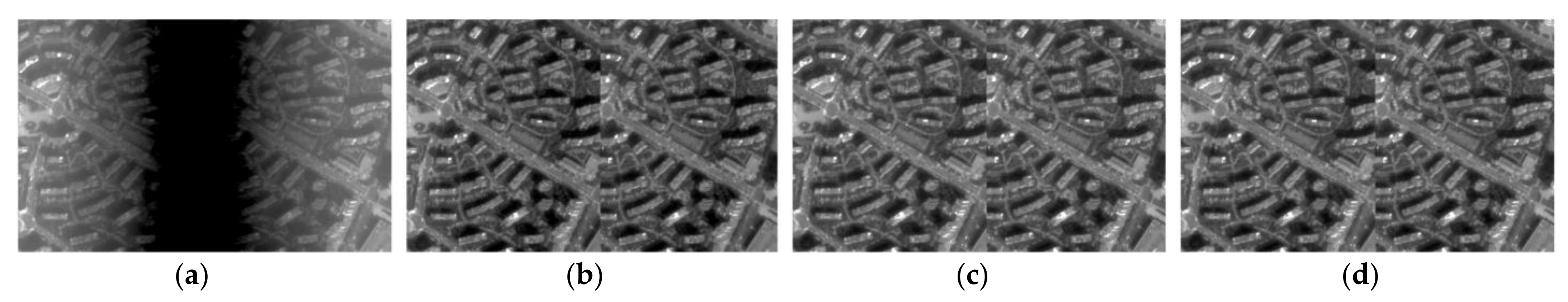
Figure 17. Raw and corrected images of the city. (a) Raw image; (b) corrected using histogram matching; (c) corrected using correction of the vignetting of multiple CCDs; (d) corrected using the proposed method.

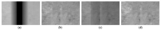
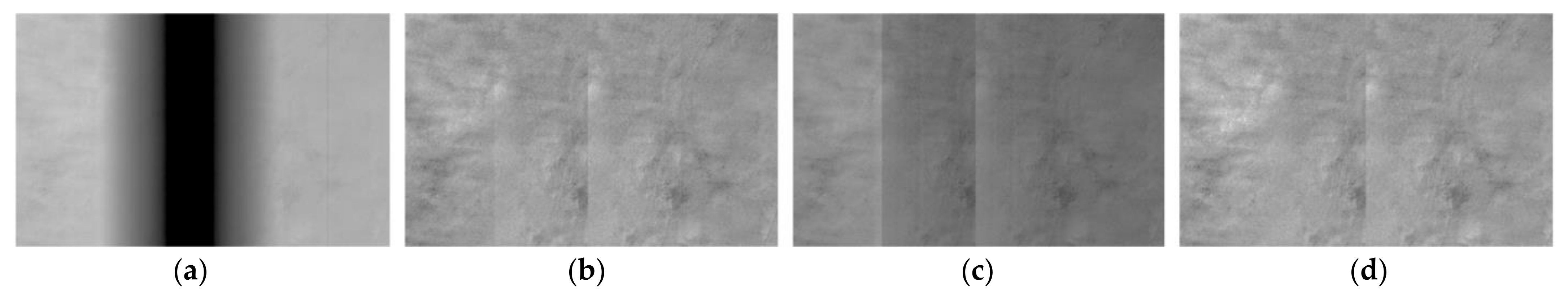
Figure 18. Raw and corrected images of the desert. (a) Raw image; (b) corrected using histogram matching; (c) corrected using correction of the vignetting of multiple CCDs; (d) corrected using the proposed method.

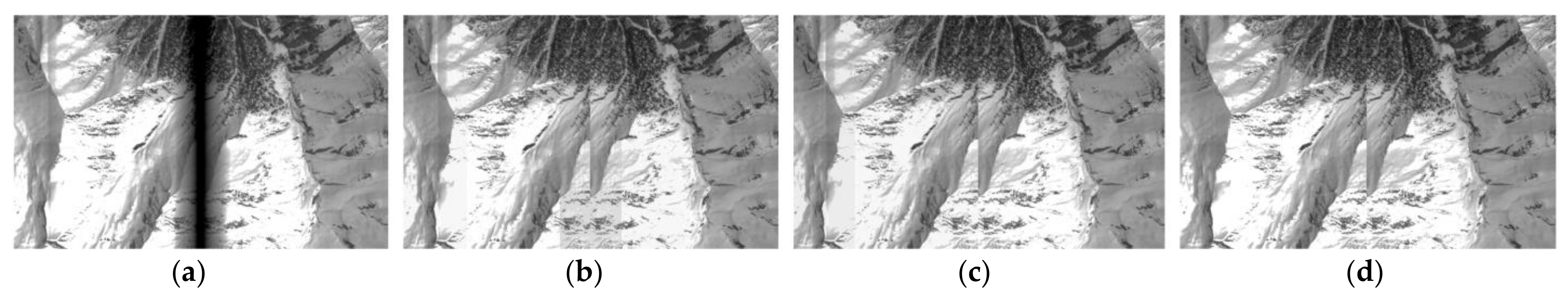
Figure 19. Raw and corrected images of the snow. (a) Raw image; (b) corrected using histogram matching; (c) corrected using correction of the vignetting of multiple CCDs; (d) corrected using the proposed method.

The original images of the water and vegetation are shown in Figure 15a and Figure 16a, and the images corrected by histogram matching are shown in Figure 15b and Figure 16b. It can be seen that the effect of histogram matching is poor. This is because the method does not consider the noise of vignetting, and it would bring in the noise of another sensor when adding the response of the corresponding points. Because of the low response of the two object features, the difference between vignetting and non-vignetting is significant. The results of vignetting and the chromatic aberration of multiple CCDs are shown in Figure 15c and Figure 16c. The right sensor has a good correction effect, and the other sensor is bad. The stripe in the transition area is between vignetting and non-vignetting. This is because the method does not consider the noise drift of each pixel of vignetting, and the response at the edge of the vignetting of the left sensor is extremely low. The method cannot effectively restore the response at the edge of vignetting. So, the correction effect of this method is limited. The results of the proposed method are shown in Figure 15d and Figure 16d and are better than the other two methods. The response of vignetting is consistent, and there is no difference between vignetting and non-vignetting. This is because we eliminate the noise drift of vignetting, which improves the stability of the pixels so that histogram matching has a better effect.

The original image corrected by histogram matching, the correction of vignetting, the chromatic aberration of multiple CCDs, and the proposed method are shown in Figure 17a–d. All three methods achieved good visual effects, and RA, SM, and RSVN are close. This is because the response of the city is high, the proportion of noise is relatively low, and the surface feature of the city is complex. The original images of the desert and snow are shown in Figure 18a and Figure 19a. The images corrected by histogram matching are shown in Figure 18b and Figure 19b. Histogram matching does not solve the problem of pixel response stability, and the effect of two object features is better than water, but there are still significant response differences and stripes between vignetting and non-vignetting. The results of vignetting and the chromatic aberration of multiple CCDs are shown in Figure 18c and Figure 19c. The response difference in the right sensor is low, and the left sensor is high. This is because the distribution of vignetting in the two sensors of the Jilin-1 GF03D satellite is not the same. The left sensor is larger, and the right is smaller. So, the energy loss of the left sensor is larger than the right one. So, the method is unable to effectively restore the response of the left sensor. The results of the proposed method are shown in Figure 18d and Figure 19d. The proposed method eliminates the noise drift of vignetting without losing image details. So, we achieved good correction results with a high response and effectively restored the response of object features of vignetting.

We select 10 image blocks, each measuring 400 × 400 pixels, from 15,927 images captured during 1,031 imaging tasks by the Jilin-1 GF03D28 satellite. These blocks are utilized to evaluate the effectiveness of the methods, and the results are shown in Table 3 and Figure 20. The mean values of RA, SM, and RSVN presented in Table 3 represent the average metrics across these 10 image blocks. The RA values of water, vegetation, and desert are 0.2652%, 1.3231%, and 0.9044%, respectively, the streaking metric values are all less than 3%, and the RSVN values obtained using the proposed method are 1.3147, 5.0059, and 5.5105, which are significantly lower than the other methods. Lower RA and SM prove better texture uniformity, while lower RSVN proves better response consistency between vignetting and non-vignetting.

Table 3. Comparison of the accuracy assessment index for the relative radiometric correction images by a quantitative sample set.

Object Features	Block	Methods	RA (%)	SM (%)	RSVN
Water	10	Histogram matching	2.2636	1.2905	2.6082
		Correction of the vignetting of multiple CCDs	0.8645	1.2643	2.5420
		Proposed method	0.2652	1.1254	1.3147
Vegetation	10	Histogram matching	2.3512	3.0824	5.3877
		Correction of the vignetting of multiple CCDs	1.4788	2.7696	5.3306
		Proposed method	1.3231	2.6626	5.0059
Desert	10	Histogram matching	2.2443	1.2386	7.1620
		Correction of the vignetting of multiple CCDs	0.9444	1.1832	5.7892
		Proposed method	0.9044	1.1671	5.5105

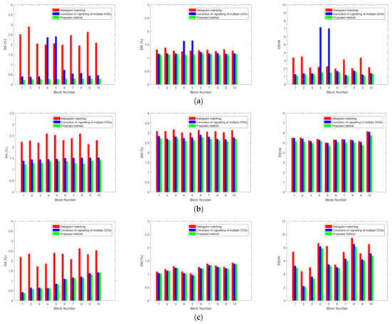
Figure 20. RA, SM, and RSVN: (a) water; (b) vegetation; (c) desert.

In summary, the proposed method can eliminate noise drift and improve the stability of the response of vignetting. Good correction results were achieved in low, medium, and high responses, and the difference between vignetting and non-vignetting was eliminated, which was better than the other methods.

4.3. Evaluation of Generality

This paper uses the CAM, which is based on multi-spectral data, to evaluate the generality of the proposed method. We selected 30 global targets of the Jilin-1 GF03D satellite randomly, which included mountains, water, deserts, etc. The results are shown in Table 4. Because of vignetting, the CAM of the raw image is extremely low. The CAM of histogram matching is relatively high, but it is basically still less than 600, which represents that there is still a stripe in the images. The CAM of the proposed method is higher than raw and histogram matching, which indicates that it eliminates the noise and noise drift in multi-spectral data. Also, this proves that it has good generality in full dynamic response intervals and multiple object features.

Table 4. Results of the CAM of global targets.

Object Feature	Target Number	Mean of Raw (CAM)	Mean of Histogram Matching (CAM)	Mean of Proposed Method (CAM)
Mountain	3	118	504	1038
Water	7	77	353	901
Desert	2	55	486	820
Cloud	2	55	208	789
Farmland	5	64	451	917
Bare Soil	4	60	291	968
City	2	69	365	912
Vegetation	4	66	399	996
Snow	1	51	513	883

The CAM results are all greater than 600 in 9 types of object features. The results indicate that the proposed method achieved a good effect in both panchromatic and multi-spectral data and also prove that good relative radiometric correction effects have been achieved within the multiple object features and full dynamic response range.

We use 56,843 images from 16 satellites in the Jilin-1 GF03D series satellites for statistics and evaluation. Compared with histogram matching, the proposed method has improved the quality of the corrected radiometric products of each satellite, as shown in Table 5. The lowest is the Jilin-1 GF03D16 satellite, with an increased rate of 11.96%, and the highest is the Jilin-1 GF03D29 satellite, with an increased rate of 19.67%. The average increasing rate is 15.97% for the 16 satellites. The generality of the proposed method for the multiple object features and full dynamic response range is verified by massive data.

Table 5. Comparison of accuracy assessment index for the relative radiometric correction images by massive data.

Satellite	Scene Number	Histogram Matching (%) (CAM $\ge$ 600)	Proposed Method (%) (CAM $\ge$ 600)	Improvement Ratio (%)
JL1GF03D01	3331	75.36	91.10	15.74
JL1GF03D03	5686	74.30	93.42	19.12
JL1GF03D05	3058	78.67	92.42	13.75
JL1GF03D07	4529	78.12	90.78	12.66
JL1GF03D11	732	73.58	90.75	17.18
JL1GF03D12	5729	75.31	88.62	13.31
JL1GF03D13	826	81.59	96.80	15.21
JL1GF03D14	3516	76.43	93.25	16.82
JL1GF03D15	3536	81.83	98.03	16.20
JL1GF03D16	2477	81.14	93.09	11.96
JL1GF03D17	3459	73.42	91.62	18.20
JL1GF03D18	3109	81.39	97.55	16.16
JL1GF03D27	2959	74.16	88.52	14.36
JL1GF03D28	3536	77.18	92.78	15.61
JL1GF03D29	6607	78.20	97.87	19.67
JL1GF03D30	3753	74.62	94.13	19.51

5. Conclusions

This paper proposes a relative radiometric correction method for vignetting optical splicing satellites. First, a vignetting stability analysis method based on the energy distribution of corresponding points was proposed, which proved that the instability of the vignetting response came from vignetting noise. Second, we used 16 Jilin-1 GF03D satellites to obtain vignetting noise data. Third, eliminate noise through the DDSN and establish a noise drift model for vignetting. Finally, automatic relative radiometric correction was completed using histogram matching. The experimental results are as follows:

(1)

A total of 1031 imaging tasks and 15,927 images of the JL1GF03D28 satellite were used to verify the effectiveness of the noise drift model for vignetting. The response stability was improved by 37.64% in the experiments. Moreover, the maximum deviation of the positions of the corresponding points closest to 50% energy was optimized from eight pixels to four pixels.

(2)

Three types of object features were used to verify the effect of the proposed method. The RA values of water, vegetation, and desert were 0.27%, 1.32%, and 0.90%, respectively, the streaking metric values were all less than 3%, and the RSVN values obtained using the proposed method were 1.31, 5.01, and 5.51, which were significantly lower than the existing methods.

(3)

A total of 56,843 images from 16 Jilin-1 GF03D satellites were used to verify the generality of the proposed method. The CAM results of the experiments show that the average rate is about 93.17%, and the average increasing rate is 15.97%.

To sum up, the proposed method can effectively solve the problem of relative radiometric correction of the vignetting of optical splicing remote sensing satellites. It eliminates the noise and noise drift and improves the stability of the pixels of vignetting. Good relative radiometric correction results were achieved in massive data, full dynamic intervals, and complex object features.

References

- Peng, X.; Zhong, R.; Li, Z.; Li, Q. Optical Remote Sensing Image Change Detection Based on Attention Mechanism and Image Difference. IEEE Trans. Geosci. Remote Sens. 2020, 59, 7296–7307. [Google Scholar] [CrossRef]
- Zhou, X.; Liu, H.; Li, Y.; Ma, M.; Liu, Q.; Lin, J. Analysis of the influence of vibrations on the imaging quality of an integrated TDICCD aerial camera. Opt. Express 2021, 29, 18108–18121. [Google Scholar] [CrossRef] [PubMed]
- Pan, J.; Ye, G.; Zhu, Y.; Song, X.; Hu, F.; Zhang, C.; Wang, M. Jitter Detection and Image Restoration Based on Continue Dynamic Shooting Model for High-Resolution TDI CCD Satellite Images. IEEE Trans. Geosci. Remote Sens. 2020, 59, 4915–4933. [Google Scholar] [CrossRef]
- Saeed, N.; Guo, S.; Park, K.H.; Al-Naffouri, T.Y.; Alouini, M.S. Optical camera communications: Survey, use cases, challenges, and future trends. Phys. Commun. 2019, 37, 100900. [Google Scholar]
- Li, Z.; Hou, W.; Hong, J.; Zheng, F.; Luo, D.; Wang, J.; Gu, X.; Qiao, Y. Directional Polarimetric Camera (DPC): Monitoring aerosol spectral optical properties over land from satellite observation. J. Quant. Spectrosc. Radiat. Transf. 2018, 218, 21–37. [Google Scholar] [CrossRef]
- Jiao, N.; Wang, F.; Chen, B.; Zhu, J.; You, H. Pre-Processing of Inner CCD Image Stitching of the SDGSAT-1 Satellite. Appl. Sci. 2022, 12, 9693. [Google Scholar]
- Alvarez-Vanhard, E.; Corpetti, T.; Houet, T. UAV & satellite synergies for optical remote sensing applications: A literature review. Sci. Remote Sens. 2021, 3, 100019. [Google Scholar]
- Sheffield, J.; Wood, E.F.; Pan, M.; Beck, H.; Coccia, G.; Serrat-Capdevila, A.; Verbist, K. Satellite Remote Sensing for Water Resources Management: Potential for Supporting Sustainable Development in Data-Poor Regions. Water Resour. Res. 2018, 54, 9724–9758. [Google Scholar]
- Liu, H.; Wang, P.; Liu, C.; Zhu, H.; Xu, S. Application and research of the accuracy calibration and detection instrument for installation of dual imaging module for aerial camera. In Proceedings of the 2017 IEEE 2nd Information Technology, Networking, Electronic and Automation Control Conference (ITNEC), Chengdu, China, 15–17 December 2017. [Google Scholar]
- Shi, Y.; Wang, S.; Zhou, S.; Kamruzzaman, M.M. Study on Modeling Method of Forest Tree Image Recognition Based on CCD and Theodolite. IEEE Access 2020, 8, 159067–159076. [Google Scholar] [CrossRef]
- Qiu, M.; Ma, W. Optical butting of linear infrared detector array for pushbroom imager. In Proceedings of the Second International Conference on Photonics and Optical Engineering, Xi’an, China, 28 February 2017; Volume 10256. [Google Scholar]
- Honkavaara, E.; Khoramshahi, E. Radiometric Correction of Close-Range Spectral Image Blocks Captured Using an Unmanned Aerial Vehicle with a Radiometric Block Adjustment. Remote Sens. 2018, 10, 256. [Google Scholar] [CrossRef]
- Liu, Y.; Long, T.; Jiao, W.; He, G.; Chen, B.; Huang, P. Vignetting and Chromatic Aberration Correction for Multiple Spaceborne CCDS. In Proceedings of the 2021 IEEE International Geoscience and Remote Sensing Symposium IGARSS, Brussels, Belgium, 12–16 July 2021. [Google Scholar]
- Goossens, T.; Geelen, B.; Lambrechts, A.; Van Hoof, C. A vignetting advantage for thin-film filter arrays in hyperspectral cameras. arXiv 2020, arXiv:2003.11983. [Google Scholar]
- Cui, H.; Zhang, L.; Li, W.; Yuan, Z.; Wu, M.; Wang, C.; Ma, J.; Li, Y. A new calibration system for low-cost Sensor Network in air pollution monitoring. Atmos. Pollut. Res. 2021, 12, 101049. [Google Scholar] [CrossRef]
- Zhang, G.; Li, L.; Jiang, Y.; Shen, X.; Li, D. On-Orbit Relative Radiometric Calibration of the Night-Time Sensor of the LuoJia1-01 Satellite. Sensors 2018, 18, 4225. [Google Scholar] [CrossRef] [PubMed]
- Moghimi, A.; Sarmadian, A.; Mohammadzadeh, A.; Celik, T.; Amani, M.; Kusetogullari, H. Distortion robust relative radiometric normalization of multitemporal and multisensor remote sensing images using image features. IEEE Trans. Geosci. Remote Sens. 2021, 60, 1–20. [Google Scholar] [CrossRef]
- Li, J.; Zhao, J.K.; Chang, M.; Hu, X.R.; Li, J. Radiometric calibration of photographic camera with a composite plane array CCD in laboratory. Guangxue Jingmi Gongcheng/Opt. Precis. Eng. 2017, 25, 73–83. [Google Scholar]
- Duan, Y.; Chen, W.; Wang, M.; Yan, L. A Relative Radiometric Correction Method for Airborne Image Using Outdoor Calibration and Image Statistics. IEEE Trans. Geosci. Remote Sens. 2013, 52, 5164–5174. [Google Scholar] [CrossRef]
- Helder, D.L.; Basnet, B.; Morstad, D.L. Optimized identification of worldwide radiometric pseudo-invariant calibration sites. Can. J. Remote Sens. 2010, 36, 527–539. [Google Scholar] [CrossRef]
- Jiang, J.; Zhang, Q.; Wang, W.; Wu, Y.; Zheng, H.; Yao, X.; Zhu, Y.; Cao, W.; Cheng, T. MACA: A Relative Radiometric Correction Method for Multiflight Unmanned Aerial Vehicle Images Based on Concurrent Satellite Imagery. IEEE Trans. Geosci. Remote Sens. 2022, 60, 1–14. [Google Scholar]
- Li, Y.; Zhang, B.; He, H. Relative radiometric correction of imagery based on the side-slither method. In Proceedings of the 2017 2nd International Conference on Multimedia and Image Processing (ICMIP), Wuhan, China, 17–19 March 2017. [Google Scholar]
- Chen, C.; Pan, J.; Wang, M.; Zhu, Y. Side-Slither Data-Based Vignetting Correction of High-Resolution Spaceborne Camera with Optical Focal Plane Assembly. Sensors 2018, 18, 3402. [Google Scholar]
- Cheng, X.-Y.; Zhuang, X.-Q.; Zhang, D.; Yao, Y.; Hou, J.; He, D.-G.; Jia, J.-X.; Wang, Y.-M. A relative radiometric correction method for airborne SWIR hyperspectral image using the side-slither technique. Opt. Quantum Electron. 2019, 51, 105. [Google Scholar] [CrossRef]
- Tan, K.C.; Lim, H.S.; MatJafri, M.Z.; Abdullah, K. A comparison of radiometric correction techniques in the evaluation of the relationship between LST and NDVI in Landsat imagery. Environ. Monit. Assess. 2012, 184, 3813–3829. [Google Scholar] [CrossRef] [PubMed]
- Liu, Y.; Long, T.; Jiao, W.; Du, Y.; He, G.; Chen, B.; Huang, P. Automatic segment-wise restoration for wide irregular stripe noise in SDGSAT-1 multispectral data using side-slither data. Egypt. J. Remote Sens. Space Sci. 2023, 26, 747–757. [Google Scholar] [CrossRef]
- Cao, B.; Du, Y.; Liu, Q.; Liu, Q. The improved histogram matching algorithm based on sliding windows. In Proceedings of the 2011 International Conference on Remote Sensing, Environment and Transportation Engineering, Nanjing, China, 24–26 June 2011. [Google Scholar]
- Shapira, D.; Avidan, S.; Hel-Or, Y. Multiple histogram matching. In Proceedings of the 2013 IEEE International Conference on Image Processing, Melbourne, Australia, 15–18 September 2013. [Google Scholar]
- Wu, Y.; Yang, P. Chebyshev polynomials, moment matching, and optimal estimation of the unseen. Ann. Stat. 2019, 47, 857–883. [Google Scholar] [CrossRef]
- Li, J.; Zhang, J.; Chen, F.; Zhao, K.; Zeng, D. Adaptive material matching for hyperspectral imagery destriping. IEEE Trans. Geosci. Remote Sens. 2022, 60, 1–20. [Google Scholar]
- Liu, Y.; Long, T.; Jiao, W.; He, G.; Chen, B.; Huang, P. A General Relative Radiometric Correction Method for Vignetting and Chromatic Aberration of Multiple CCDs: Take the Chinese Series of Gaofen Satellite Level-0 Images for Example. IEEE Trans. Geosci. Remote Sens. 2022, 60, 1–25. [Google Scholar] [CrossRef]
- Li, L.; Li, Z.; Wang, Z.; Jiang, Y.; Shen, X.; Wu, J. On-Orbit Relative Radiometric Calibration of the Bayer Pattern Push-Broom Sensor for Zhuhai-1 Video Satellites. Remote Sens. 2023, 15, 377. [Google Scholar] [CrossRef]
Disclaimer/Publisher’s Note: The statements, opinions and data contained in all publications are solely those of the individual author(s) and contributor(s) and not of MDPI and/or the editor(s). MDPI and/or the editor(s) disclaim responsibility for any injury to people or property resulting from any ideas, methods, instructions or products referred to in the content. |
© 2023 by the authors. Licensee MDPI, Basel, Switzerland. This article is an open access article distributed under the terms and conditions of the Creative Commons Attribution (CC BY) license (https://creativecommons.org/licenses/by/4.0/).